Bayesian Integrated Nested Laplace Approximation (INLA) Longevity Bonds Market Model

Abstract

Pricing coupon longevity bonds (CLBs) is challenging in illiquid markets due to the incompleteness of insurance markets and the unavailability of longevity payout data. In addition, pension funds may experience significant surges in annual mortality-improvement reserves (MIRs), consistent with systematic longevity drift and cohort-survival effects. We propose a Bayesian pricing model based on the Integrated Nested Laplace Approximation (INLA) for CLBs in pension-fund applications. The term structure of interest rates is modeled using a two-factor Cox–Ingersoll–Ross (CIR) specification, while mortality dynamics are captured using a CIR affine jump–diffusion model to capture abrupt longevity shocks. Posterior inference is performed via INLA and benchmarked against Markov chain Monte Carlo (MCMC). Using South African government bond yield data, pension-fund MIR series, and population survival-rate reports, we show that INLA provides a computationally efficient approximation to the MCMC posterior with substantially reduced computation time. Longevity Greeks derived from the model support hedge construction and evaluation of strategies aimed at mitigating rising longevity-linked cash flows. Empirically, model-implied longevity payouts are positively skewed with high dispersion and exhibit frequent jump episodes over a broad range, underscoring the importance of jump risk in CLB valuation and hedging.

1. Introduction

Most pensioners, in their twilight years, live beyond the retirement fund capacity (known as longevity risk). The longevity-linked-securities’ market is driven by the demand for a stable annuitized income stream that guarantees the payout of capital. Our choice of instrument is the coupon longevity bond that earns annuitized coupon payments, which begin at a high value and decline over time until maturity, while being dependent upon the underlying risk factors such as the stochastic processes of mortality and interest rates (Menoncin 2008; Xu et al. 2024). Consequently, a huge proportion of this cohort of pensioners can survive longer than anticipated, and that may result in an increase in coupon rates and thus offset the issuer’s costs to a deficit.

There is a plethora of longevity bond classifications in Blake et al. (2006), and the classifications are limited to two broad types. The primary type comprises principal-at-risk longevity bonds, like the Swiss Re mortality bond, where the pensioner will be entitled to partial or zero principal. The secondary type are coupon-based longevity bonds. In this paper, we considered a hybrid type called the coupon longevity bond (CLB), wherein both the coupons and their principal values are subject to longevity market price risk in the event of a payout (Menoncin 2008). In the Bayesian literature, the Lee–Carter model, as a one-factor model, has been criticized for inconsistencies, such as using a single parameter to capture all ages, which may not be appropriate for our model due to its limited ability to capture age-period-cohort (APC) dynamics (Fushimi and Kogure 2014). Moreover, in the paper by Shi et al., it is noticeable that Lee and Carter rely on linear time-series dynamics and struggles to capture nonlinear jumps like the COVID-19 pandemic shock (Shi et al. 2025). In order to price longevity-linked securities accurately, we consider the use of the two-factor Cox–Ingersoll–Ross (CIR) affine jump–diffusion (which enables us to capture mortality shocks) and the Renshaw–Haberman (RH) models. Thus, in this paper, we employ the RH model, which outperforms Lee–Carter, as it has the inborn feature of APC that ameliorates the longevity risk forecasts in pensions and insurance models (Renshaw and Haberman 2006).

In portfolio diversification and the management of longevity risk, a benchmarking strategy is to package capital reserves according to Solvency II (a comprehensive European Union regulatory framework for insurance and reinsurance companies, effective since January 2016) to mitigate extra deficits incurred in the underestimation of longevity risk (Leung et al. 2018; Olivieri and Pitacco 2008; Zeddouk and Devolder 2019). Various reputable pricing approaches were investigated that have been previously proposed in the literature, like the risk-neutral, Wang transform, canonical valuation, economic tatonnement, and utility indifference pricing method (Leung et al. 2018). The sampling-based Bayesian approach was employed for the distribution of the longevity risk-premiums (Leung et al. 2018). Carter and Kohn (1994) used an estimation method such as the Markov chain Monte Carlo (MCMC) for real-life modeling and forecasting under the Bayesian framework. Leung et al. (2018) provided a state-space mortality model reliant on the Cairns–Blake–Dowd (CBD) model that tackles parameter uncertainty and longevity valuation of instruments. In this paper, we construct a Bayesian state-space representation that uses the CIR affine-jump diffusion and Renshaw–Haberman model to contribute to literature by enabling the mortality parameter to handle age-specific cohorts, while the interest rate parameter handles the illiquidity risk and inflation. Enshrining the affine jump–diffusion feature into the mortality model enables us to fit empirical data, such as pandemics, medical breakthroughs, and general geopolitical shocks that have an impact on mortality rate dynamics (Guo and Li 2025; Liu et al. 2014; Xu et al. 2024). Furthermore, by employing the Bayesian integrated Laplace approximation (INLA) algorithm, we are able to hedge illiquidity risk and inflation and to generate fairly priced (arbitrage-free) premiums for an incomplete market. It is evident in the paper by Sahin and Levitan that it is crucial to take inflationary pressures into account when constructing pension fund models for life insurance firms in South Africa for the period 2000–2018 (Sahin and Levitan 2021). Moreover, the work of Takadong shows that the South African pension fund market is characterized by illiquidity, as inflation-linked products are only available over-the-counter (OTC), and a government firm like GEPF is the main issuer of pension funds (Takadong 2009). Additionally, mortality improvements are surging globally and exerting pressure on government entities like GEPF and the life insurance firms to buffer and hedge increasing longevity risk (Blake and Cairns 2025). Thus, in this paper, we demonstrate that Bayesian INLA applied to CLB pricing embeds a stochastic mortality forecasting model that accounts for unprecedented shocks within a posterior estimation framework that attenuates the compounded risks of illiquidity and inflation.

As stated by (Martino and Riebler 2019; Martino and Rue 2009), INLA is a fast distribution model in Bayesian inference for latent Gaussian models (LGMs) compared to the computationally demanding MCMC. To obtain precise estimations for the posterior, INLA has shown itself to be reliant on a parsimonious integration approach. Therefore, we present the Bayesian belief filtering mechanism to recursively give a consistent pricing model through the updating of INLA beliefs. This provides inference on price data intervals given a set of latent parameters. Furthermore, in the literature, it is noteworthy that axiomatic belief propagations are not enshrined in INLA’s approximation approach and are rather applied in broader Bayesian networks or belief functions such as Sjenoy’s framework (Shenoy and Shafer 1990). Thus, our investigation in the literature shows, despite the paper we wrote about the assessment of geopolitical risk on longevity bond pricing by Sithole et al. (2024), no other studies have applied INLA to develop a pricing process for longevity risk, despite the application of a Bayesian ensemble approach to the pricing of participating longevity-linked life annuities by Bravo (2022). Therefore, we explore the INLA approach backed by an axiomatic belief mechanism and avoid the computationally heavy MCMC approach and relaxed Bayesian methods like the variational inference (or variational dropout) approach, which utilizes minimization of the Kullback–Leibler divergence or the maximization of the evidence lower bound (Bhattacharya and Wilson 2015; Martin et al. 2019; Ruiz-Cárdenas et al. 2010). As the inclusion of an axiomatic belief mechanism within the INLA frameworks promotes the interpretability, rigor, and theoretical guarantees for approximate Bayesian inference in LGMs.

The main result presented in this paper is the formulation of a Bayesian state-space model for the incomplete market that allows for accurate pricing of longevity bonds. This niche market is susceptible to various shocks (e.g., geopolitical risk, pandemics, health breakthroughs, etc.), and our model accounts for that. We utilize a hybrid-type coupon longevity bond (CLB) that includes coupons and principal values, which are contingent on longevity risk markets. We have also extended the state parameter in vector form so that it handles the age-specific cohort mortalities and the interest rates associated with illiquidity risk independently. To do this, we utilize a joint-state CIR-AJD Renshaw–Haberman model, which encapsulates the interest and mortality rates. Lastly, we employ the Bayesian INLA algorithm, which has a faster convergence rate (based on our findings) than the MCMC in generating CLB prices through the marginal posterior distribution.

The outline of the paper is structured as follows: in the next section, we present the coupon longevity bond pricing preliminaries, wherein we provide a pricing kernel that takes into account the bid-ask spread, government bond price, and survival probabilities. In Section 3, we present a discretized CIR-AJD Renshaw–Haberman state-space through an INLA-ready jump-adjusted discretization scheme. In Section 4, we demonstrate how a Bayesian state-space is constructed and justify why MCMC is computationally expensive, as it incites the curse of dimensionality due to the intractability of the evidence term. In Section 5, we give a detailed Bayesian INLA pricing framework with a filtration process that makes use of an axiomatic belief mechanism under the conjugacy assumption. In Section 6, we construct the INLA incomplete market model and illustrate that the market is capable of propagating fair longevity risk premiums. In Section 7, we provide the analysis and results of the study and discuss the conclusions in the last section.

2. Preliminaries for the Coupon Longevity Bond Pricing Framework

In this section, we define the CLB instrument and set up its specifications by developing a state-space representation necessary for the construction of a Bayesian pricing system. Our work is also self-contained in the sense that we present the basic construct of the CLB that has an underlying deterministic function of time, comprising interest rate and stochastic mortality intensity. We consider an instantaneous short rate $r\left(t\right)$ as a two-factor model given by

$$r\left(t\right)=\varpi \left(t\right)-[\vartheta \left(t\right)+r_1\left(t\right)+r_2\left(t\right)],$$

(1)

where $\varpi \left(t\right)$ represents the long-run mean rate, $\vartheta \left(t\right)$ is the deterministic function of time, and the unobservable latent factors $r_1\left(t\right)$ and $r_2\left(t\right)$ represent illiquidity risk and inflation, respectively Ikpe et al. (2022). Here, the dynamics of the interest rate ${\theta }_r=r\left(t\right)$ are governed by the stochastic differential Equation (SDE), known as the two-factor Cox–Ingersoll–Ross (CIR) model with an underlying martingale measure ${\mathbb{P}}_1$, given as

$$\begin{array}{c}d{r}_1\left(t\right)=k_{r_1}({\gamma }_r-r_1\left(t\right))dt+{\sigma }_{r_1}\sqrt{r_1\left(t\right)}d{W}_{r_1}^{{\mathbb{P}}_1}\left(t\right),\\ d{r}_2\left(t\right)=k_{r_2}({\gamma }_r-r_2\left(t\right))dt+{\sigma }_{r_2}\sqrt{r_2\left(t\right)}d{W}_{r_2}^{{\mathbb{P}}_1}\left(t\right).\end{array}$$

(2)

The dynamics of mortality intensity ${\theta }_{\lambda }=\lambda \left(t\right)$ are captured by the Renshaw–Haberman (RH) model in exponential form as follows:

$${\lambda }^i\left(t\right)=exp\{{\alpha }_x+{\beta }_x{\kappa }_{\lambda }+c_x{\gamma }_{t-x}^i+{\omega }_{\lambda k}\},$$

(3)

such that its natural logarithmic form is given by

$$ln{\lambda }^i\left(t\right)={\alpha }_x+{\beta }_x{\kappa }_{\lambda }+c_x{\gamma }_{t-x}^i+{\omega }_{\lambda k},$$

(4)

with constraints,

$$\begin{array}{ccc}\sum {\beta }_x=\sum c_x=1,& \mathrm{and}& \sum {\kappa }_x=\sum {\gamma }_{t-x}^i=0,\end{array}$$

(5)

where ${\alpha }_x$ represents the age trend of mortality rates, the ${\beta }_x$ represents age-specific reactions to the time-varying sensitivity, $c_x$ represents the sensitivity of the log central death rate at each age to cohort effects, ${\kappa }_x$ is an age-dependent period effects factor, ${\gamma }_{t-x}^i$ is the cohort-specific stochastic factor linked to year-of-birth $(t-x)$, and ${\omega }_{\lambda k}$ is the mortality estimation error term (Chen and Cox 2009; Guo and Li 2025). The dynamics of ${\kappa }_x$ are governed by an affine-diffusion process given by

$$d{\kappa }_x=-g_1{\kappa }_{x}dt+{\sigma }_{1}d{W}_1^{{\mathbb{P}}_2},$$

(6)

where $g_1,{\sigma }_1\in \mathbb{R}$, and $\{W_1^{{\mathbb{P}}_2}\left(t\right):t>0\}$ is the benchmark Brownian motion under the probability measure ${\mathbb{P}}_2$. Additionally, the cohort-specific stochastic factor is driven by an affine jump–diffusion process given by

$$d{\gamma }_{t-x}^i=-g_2^i{\gamma }_{t-x}^{i}dt+{\sigma }_2^{i}d{W}_2^{{\mathbb{P}}_2,i}\left(t\right)+d{\displaystyle \sum _{k=1}^{N^{{\mathbb{P}}_1,i}\left(t\right)}}{\mathbf{J}}_k^i,$$

(7)

where $g_2^i,{\sigma }_2^i\in \mathbb{R}$, $N^{{\mathbb{P}}_2,i}\left(t\right)$ is a Poisson process with intensity ${\eta }^1({\eta }^1>0)$ under the probability measure ${\mathbb{P}}_2$, and $\{{\mathbf{J}}_{k=1}^i,k=1,2,\dots \}$ are i.i.d random variables (Xu et al. 2024). Based on the Girsanov theorem with an underlying risk-neutral longevity risk pricing measure $\mathbb{Q}\left({\phi }_R\right)$ we have the following Brownian motions,

$$\begin{array}{c}d{W}_1^{\mathbb{Q}\left({\phi }_R\right)}=d{W}_1^{{\mathbb{P}}_2}+{\phi }_1\left(t\right)dt,\\ d{W}_2^{\mathbb{Q}\left({\phi }_R\right)}=d{W}_2^{{\mathbb{P}}_2}+{\phi }_2^i\left(t\right)dt.\end{array}$$

(8)

Moreover, we model mortality by using the affine jump–diffusion (AJD) age-specific-cohort model due to its ability to accurately fit empirical data (sudden jumps like pandemics, geopolitical risk shocks, and medical breakthroughs) (Liu et al. 2014; Xu et al. 2024), given by

$$\begin{array}{c}\hfill d{\lambda }_x^i\left(t\right)=[-g_1{\kappa }_x-g_2^i{\gamma }_{t-x}^i-{\sigma }_1{\phi }_1-{\sigma }_2^i{\phi }_2^i]dt\\ \hfill +{\sigma }_{1}d{W}^{\mathbb{Q}\left({\phi }_R\right)}\left(t\right)+{\sigma }_2^{i}d{W}_2^{\mathbb{Q}\left({\phi }_R\right),i}\left(t\right)+d{\displaystyle \sum _{k=1}^{N^{\mathbb{Q}\left({\phi }_R\right),i}\left(t\right)}}{\mathbf{Y}}_k^i,\end{array}$$

(9)

where the vector ${\phi }_{\mathbf{R}}=({\phi }_1,{\phi }_2)$ denotes the market prices of longevity risk, and y is the jump realization. Furthermore, according to the definition of the Poisson random measure, the last term of Equation (9) given in discrete form can be written in continuous integral form as follows:

$$d{\displaystyle \sum _{k=1}^{N^{\mathbb{Q}\left({\phi }_R\right),i}\left(t\right)}}{\mathbf{Y}}_k^i={\int }_{\mathbf{R}}y{N}^{\mathbb{Q}\left({\phi }_R\right),i}(dt,dy),$$

(10)

where $N^{\mathbb{Q}\left({\phi }_R\right),i}(dt,dy)$ is the correlated Poisson random measure of Equation (10), and ${\nu }^{\mathbb{Q}\left({\phi }_R\right),i}\left(dy\right)$ is the compensator of $N^{\mathbb{Q}\left({\phi }_R\right),i}(dt, dy)$ (Xu et al. 2024).

Discretization of the CIR-AJD SDE and Pricing Kernel of the CLB

The CIR-AJD is a continuous-time homogeneous construct that runs forever with indefinite detail. Discretizing the SDE transforms it into a sequence of simple update rules that chop up time into finite steps, $\Delta t_i$ which are like film frames, and replace infinitesimals with finite differences. Furthermore, we discretize Equation (7) (two-factor CIR rates), wherein the diffusion term $d{W}^{\mathbb{Q}}$ with the randomized volatility component is driven by the Brownian motion that has an underlying risk-neutral measure $\mathbb{Q}$:

$$\begin{array}{c}{r}_i^{\left(1\right)}-r_{i-1}^{\left(1\right)}=k_1({\theta }_1-r_{i-i}^{\left(1\right)})\Delta t_i+{\sigma }_1\sqrt{r_{i-1}^{\left(1\right)}\Delta t_i{Z}_i^{\left(1\right)}},\\ r_i^{\left(2\right)}-r_{i-2}^{\left(2\right)}=k_2({\theta }_2-r_{i-2}^{\left(2\right)})\Delta t_i+{\sigma }_2\sqrt{r_{i-2}^{\left(2\right)}\Delta t_i{Z}_i^{\left(2\right)}},\end{array}$$

(11)

with $Z_i^{(j=1,2)}\sim \mathcal{N}(0,1)$, and the $Corr(Z^{\left(1\right)},Z^{\left(2\right)})={\rho }_{1,2}$.

Moreover, discretizing Equation (9) yields the below formulation of the AJD for mortality rates in discrete form with the drift and diffusion approximation on the adaptive grid $t_{i-1}$ to $t_i$, such that $\Delta t_i=t_i-t_{i-1}$

$$\Delta {\lambda }_x^i=\left[-g_1{\kappa }_x-g_2^i{\gamma }_{t_i-x}^i-{\sigma }_1{\phi }_1-{\sigma }_2^i{\phi }_2^i\right]\Delta t_i+{\sigma }_1\sqrt{\Delta t_i}{Z}_1^i+{\sigma }_2\sqrt{\Delta t_i}{Z}_2^i,$$

(12)

where $Z_1^i,Z_2^i\sim \mathcal{N}(0,1)$, and correlated through $\mathbb{Q}\left({\phi }_R\right)$.

We define and articulate our instrument as an agreement between the issuer of securities and the pensioner as follows:

Definition 1 (Limit Zero Coupon Longevity Bond). 

A limit coupon longevity bond with an expiration date T guarantees the pensioner $1\left(ZAR\right)$ rand to be compensated on the date T. Moreover, apart from its risk-neutral rate $r\left(t\right)$, there is an extra cost arising from longevity risk that is associated with the stochastic mortality rate $\lambda \left(t\right)$. Therefore, the random price of the longevity bond agreement at the inception time t with maturity T is given by $D(t,T)$, whiles the cumulative cost for term-to-maturity is represented as $L_{\infty }(t,T)$.

Definition 2 (Coupon Longevity Bond). 

A coupon longevity bond $L(t,T)$ is defined as an agreement at time t, to pay coupons until maturity T. Here, the coupons decline in value over time and are stringently proportional to the survival rate of a cohort aged x on a term horizon. The product is targeting pensioners who are 65 years and older.

Definition 3 (Martingale measure $\mathbb{Q}$).

A probability measure $\mathbb{Q}$ is regarded as a martingale measure if the following holds:

$$L_0={\displaystyle \frac{1}{1+R}}{\mathbb{E}}^{\mathbb{Q}}\left[L_1\right],$$

where R is the risk-free rate, $L_0$ is the current coupon longevity bond price and $L_1$ is the future coupon longevity bond price (a continuous random variable).

Proposition 1 (Fundamental Theorem). 

There exists a martingale measure $\mathbb{Q}$, if and only if the coupon longevity bonds’ market model is arbitrage-free.

We consider that the interest- and mortality-rates are independent under the product probability space $\left(\Omega \times \tilde{\Omega },{\mathcal{F}}_t=\{{\mathcal{G}}_t^r\vee {\mathcal{H}}_t^{\lambda }\},\mathbb{Q}={\mathbb{P}}_1·{\mathbb{P}}_2\right)$, such that the price at time t for a coupon longevity bond with maturity T is represented as

$$\begin{array}{c}\underset{m\to \infty }{lim}{L}_{\left(m\right)}(t,T)=L_{\infty }(t,T)=e^{\delta (T-t)}·\underset{\mathrm{risk}-\mathrm{neutral}\mathrm{price}\mathrm{of}\mathrm{a}\mathrm{bond},}{\underbrace{{\mathbb{E}}_t^{{\mathbb{P}}_1}\left[e^{-{\int }_t^{T}r\left(u\right)du}|{\mathcal{G}}_t^r\right]}}·\underset{\mathrm{risk}-\mathrm{neutral}\mathrm{survival}\mathrm{probability}}{\underbrace{{\mathbb{E}}_t^{{\mathbb{P}}_2}\left[e^{-{\int }_t^T\lambda \left(u\right)du}|{\mathcal{H}}_t^{\lambda }\right]}},\\ L(t,T)=e^{\delta (T-t)}{\mathbb{E}}_t^{\mathbb{Q}\left({\phi }_R\right)}\left[e^{-{\int }_t^{T}r\left(u\right)du}{e}^{-{\int }_t^T\lambda \left(u\right)du}|{\mathcal{F}}_t\right],L(T,T)=1,\end{array}$$

(13)

where $\mathbb{Q}$ is the martingale measure, ${\phi }_R$ is the market price of longevity risk, and $\mathbb{Q}\left({\phi }_R\right)$ is a risk-neutral martingale measure for longevity premiums (a measure that will be discussed in subsequent sections) (Cairns et al. 2006). We consider the survival probability that takes into account the force of mortality given by $\lambda \left(t\right)$. The mortality intensity is a measure of how many people die in each period, expressed as

$$\begin{array}{ccc}{\displaystyle \frac{d\pi \left(t\right)}{\pi \left(t\right)}}=-\lambda \left(t\right)dt,& & \pi \left(0\right)=1.\end{array}$$

(14)

Additionally, a CLB issued at t with maturity at T under the measure $\mathbb{Q}\left({\phi }_R\right)$ with a bid-ask spread denoted by $\delta$ that has coupon payouts, which are strictly proportional to the survival rate given ${\displaystyle \frac{\pi \left(s\right)}{\pi \left(t\right)}}$ and inversely proportional to Equation (14), gives us

$$\begin{array}{c}L(t,T)=e^{\delta (T-t)}{\mathbb{E}}_t^{\mathbb{Q}\left({\phi }_R\right)}\left[e^{-{\int }_t^T\theta (r\left(u\right)du}{\displaystyle \frac{{\sum }_{i=1}^m{1}_{{\tau }^i>s}}{{\sum }_{j=1}^m{1}_{{\tau }^j>t}}}|{\mathcal{G}}_t^r\vee {\mathcal{H}}_t^{\lambda }\right]\\ L(t,T)=e^{\delta (T-t)}{\mathbb{E}}_t^{\mathbb{Q}\left({\phi }_R\right)}\left[e^{-{\int }_t^T\theta (r\left(u\right)du}{e}^{-{\int }_t^T\lambda \left(u\right))du}|{\mathcal{G}}_t^r\vee {\mathcal{H}}_t^{\lambda }\right]\end{array}$$

(15)

$$L(t,T)=e^{\delta (T-t)}P(t,T)S^{\mathbb{Q},i}(x,t,T),$$

(16)

where the dynamics of the interest rates and those of mortality rates are independent from each other. Also, the survival probability is represented as

$$S^{\mathbb{Q},i}(x,t,T)=1-q_x^i\left(t\right),$$

(17)

where the cohort i over the term interval $[t,T]$, with x representing years of age. The probability that a pensioner will die in a year is given by

$$q_x^i\left(t\right)=1-S^{\mathbb{Q},i}(x,t,T)=1-exp\{-{\int }_0^1{\lambda }_{x,t}\left(t\right)dt\}.$$

(18)

We define the central mortality rate as $m_{x,t}$ and it is computed as follows:

$$m_{x,t}={\displaystyle \frac{D(x,t)}{E(x,t)}}={\displaystyle \frac{\mathit{Death}\mathit{cases}\mathit{aged}\mathit{x}\mathit{during}\mathit{year}\mathit{t}}{\mathit{Risk}\mathit{exposure}\mathit{aged}\mathit{x}\mathit{during}\mathit{year}\mathit{t}}}$$

(19)

and since $m_{x,t}={\lambda }_x\left(t\right)$, we can represent the probability of dying of the insured aged x at year t as

$$q_x^i\left(t\right)=1-exp\{-m_{x,t}\}.$$

(20)

The mortality force for a two-factor model looks as follows

$${\lambda }_x^i\left(t\right)=m_{x,t}=exp\{{\alpha }_x+{\beta }_x{\kappa }_{\lambda }+c_x{\gamma }_{t-x}^i\},$$

(21)

where ${\theta }_k={({\theta }_r,{\theta }_{\lambda })}^T$ and the death probability is given by

$$q_x^i\left(t\right)=1-exp\{-exp\{{\alpha }_x+{\beta }_x{\kappa }_{\lambda }+c_x{\gamma }_{t-x}^i\}\}.$$

(22)

3. Discretized CIR-AJD Renshaw–Haberman State-Space

A CIR–Renshaw–Haberman vector state-space representation is presented with a Markovian sequence characteristic, such that it represents an affine joint state-transition model that has an unobservable process. Due to uncertainty in the system, there is a signal (e.g., geopolitical risk shock like tariff hikes threat) to noise (e.g., market uncertainty as a result of a shock) ratio on the price data observations such that the state-space model can be employed to address uncertainty in the system. To construct a practical state-space for our CLB market, we employ the below system of state Equations,

$$\begin{array}{c}r\left(t\right)=\underset{a_r}{\underbrace{\varpi \left(t\right)-\vartheta \left(t\right)}}-r_1\left(t\right)-r_2\left(t\right),\\ {\lambda }_x^i\left(t\right)=exp\{{\alpha }_x+{\beta }_x{\kappa }_x+c_x{\gamma }_{t-x}^i\}.\end{array}$$

(23)

Let ${\mathbf{V}}_{k1}$ denote the two-factor yield of a CLB and $ln{m}_{x,t}$ denote the observation of mortality via the Renshaw–Haberman model, such that they are represented by the below system given by

$$\begin{array}{c}{\mathbf{V}}_{k1}=a_r+b_r{r}_1+c_r{r}_2+{\omega }_{rk},\\ ln{m}_{x,t}={\alpha }_x+{\beta }_x{\kappa }_x+c_x{\gamma }_{t-x}^i+{\omega }_{\lambda k}.\end{array}$$

(24)

Furthermore, we restructure our CIR–Renshaw–Haberman state-space formulation in vector form as follows:

$$\begin{array}{c}\mathbf{Vector}\mathbf{Observation}\mathbf{Model}\\ {\mathbf{V}}_k=V_t=\left(\begin{array}{c}{\mathbf{V}}_{k1}\\ ln{m}_{x,t}\end{array}\right)=\left(\begin{array}{c}{a}_r\\ {\alpha }_x\end{array}\right)+\left(\begin{array}{c}(b_r{r}_1+c_r{r}_2)\\ ({\beta }_x{\kappa }_x+c_x{\gamma }_{t-x}^i)\end{array}\right)+\left(\begin{array}{c}{\omega }_{rk}\\ {\omega }_{\lambda k},\end{array}\right),\\ {\mathbf{V}}_k=\left(\begin{array}{c}{a}_r\\ {\alpha }_x\end{array}\right)+\left(\begin{array}{cc}1& 0\\ 0& 1\end{array}\right)\left(\begin{array}{c}{\theta }_r\\ {\theta }_{\lambda }\end{array}\right)+\left(\begin{array}{c}{\omega }_{rk}\\ {\omega }_{\lambda k},\end{array}\right),\\ \begin{array}{c}{\omega }_{rk}\sim N(0,{\sigma }_{{\omega }_r}^2),\\ {\omega }_{\lambda k}\sim N(0,{\sigma }_{{\omega }_{\lambda }}^2),\end{array}\\ \mathbf{Vector}\mathbf{State}\mathbf{Model}\\ {\theta }_k=\left(\begin{array}{c}{\theta }_r\\ {\theta }_{\lambda }\end{array}\right)=\left(\begin{array}{c}\varpi \left(t\right)-\vartheta \left(t\right)-r_1\left(t\right)-r_2\left(t\right)\\ exp\{{\alpha }_x+{\beta }_x{\kappa }_x+c_x{\gamma }_{t-x}^i\}\end{array}\right)+\left(\begin{array}{c}{ϵ}_{rk-1}\\ {ϵ}_{\lambda k-1},\end{array}\right),\\ \begin{array}{c}{ϵ}_{rk-1}\sim N(0,{\sigma }_{{ϵ}_{\overline{r}}}^2),\\ {ϵ}_{\lambda k-1}\sim N(0,{\sigma }_{{ϵ}_{\lambda }}^2),\end{array}\end{array}$$

(25)

where ${\mathbf{V}}_k={({\mathbf{V}}_{k1},ln{m}_{x,t})}^T$ represents the observation vector containing the yield parameter ${\mathbf{V}}_{k1}$ and mortality rate parameter $ln{m}_{x,t}$, ${\theta }_k={({\theta }_r,{\theta }_{\lambda })}^T$ is a two-factor state vector representing of interest rates ${\theta }_r$, and the mortality rates ${\theta }_{\lambda }$. ${\omega }_{rk}$ represents the observation noise of the CLB yields, while the error term ${\omega }_{\lambda k}$ represents the noise associated with age-specific influences not accounted for by the Renshaw–Haberman model (Chen and Cox 2009). Similarly, the terms ${ϵ}_{rk-1}$ and ${ϵ}_{\lambda k-1}$, represent state noises of the interest rates and mortality rates, respectively.

Scheme for INLA-Ready Jump-Adjusted Discretization

Now that we have discretized the CIR-AJD-SDE, we also discretize the state-space, as this equips it with the power to tractably account for unexpected shocks in the form of jumps. With the time grid given by $0=t_0<t_1<t_2<\dots <t_N=T$, and $\Delta t_k=t_k-t_{k-1}$, the discretization transforms the continuous-time SDEs into core structural foundation of INLA’s latent Gaussian model (LGM), and the Gaussian Markov random field (GMRF) framework. While maintaining the sparse accuracy of the swift Bayesian learning, each time step propagates a realistic trajectory. We present the scheme below, which consists of 5 steps that discretize our CIR-AJD-RH state-space:

1.

Firstly, we enshrine the jump detection feature via the thinning scheme, given by

$$\begin{array}{ccc}\widetilde{{\tau }_{k,j}}\sim Exp\left(\overline{\eta }\right),& & \overline{\eta }=\eta \left({\theta }_{r_k}\right),\\ p_j=min\left(1,{\displaystyle \frac{\eta \left({\theta }_{r_{k-1}}\right)}{\overline{\eta }}}\right),& & {\tau }_{k,j}=\{{\overline{\tau }}_{k,j}:U_j<p_j\}.\end{array}$$

Basically, thinning helps us address the fundamental challenge of the state-dependent jump intensity parameter $\eta \left({\theta }_{r_{k-1}}\right)$, by constructing an auxiliary homogeneous Poisson process with a constant upper bound $\overline{\eta }=\eta \left({\theta }_{r_k}\right)$, then accepting proposed jump times with probability ${\displaystyle \frac{\eta \left({\theta }_{r_{k-1}}\right)}{\overline{\eta }}}$ and rejecting the remainder (Lemaire et al. 2020). Through exploitation of the CIR ergodicity, the upper bound $\overline{\eta }=\eta \left({\theta }_{r_k}\right)$ guarantees finite anticipated proposals. The successful jump times ${\tau }_{k,j}$ are aligned precisely with the real Poisson arrivals, thus making timing bias negligible. The precise jump detection generates a Markov chain with the tridiagonal precision matrix $\Omega$, where the off-diagonals of ${\Omega }_{k,k-1}$ depend on the previous state ${\theta }_{k-1}$. The sparse structure lets INLA solve big scale datasets of decades of South African longevity data in linear time using its swift Cholesky solver (Rue et al. 2009).

2.

Secondly, we discretize the mortality state ${\lambda }_x^i\left(t\right)$ between jumps and update it at jump times so that the resulting CIR-AJD-SDE approximation can be written in a latent Markov form that is suitable for INLA. Between jump arrivals ${\tau }_{k,j}$, the continuous evolution is approximated by an Euler-Maruyama discretization of the CIR-type diffusion given by (Shen and Zhang 2025),

$${\lambda }_x^i\left(t_k\right)={\lambda }_x^i\left(t_{k-1}\right)+k_x({\mu }_x-{\lambda }_x^i\left(t_{k-1}\right))\Delta t_k+{\sigma }_{\lambda }\sqrt{{\lambda }_x^i\left(t_{k-1}\right)}\Delta W_k^i,$$

(26)

where $\Delta W_k^i=\sqrt{\Delta t_k}{Z}_k^i$ and $Z_k^i\sim \mathcal{N}(0,1)$, while ${\mu }_k$ collects the deterministic cohort and frailty drift terms. The jump arrival times are generated from the integrated intensity $\Lambda \left(t\right)={\int }_0^t\lambda \left(s\right)ds$; when the exact inversion is tractable, via the use of the standard time-change representation ${\tau }_j={\Lambda }^{-1}(E_1+E_2+\dots +E_j)$, with $E_j\stackrel{\mathrm{i}.\mathrm{i}.\mathrm{d}}{\sim }\mathrm{Exp}\left(1\right)$ a continuous memoryless distribution, an equivalent thinning-based simulation may be used. Therefore, at each arrival time ${\tau }_{k,j}$, the state receives a discontinuous increment drawn from the model’s jump kernel,

$$\begin{array}{cc}{\lambda }_x^i\left({\tau }_{k,j}^{+}\right)={\lambda }_x^i\left({\tau }_{k,j}^{-}\right)+Y_{\lambda },& Y_{\lambda }\sim {\nu }^{\mathbb{Q}\left({\phi }_R\right),i}\left(dy\right).\end{array}$$

The grid spacing $\Delta t_k$ is chosen adaptively to control the weak approximation error, following the adaptive weak stepping notion for jump diffusions. In this setup, the discretized latent state is organized to retain a sparse Markov structure that is suitable for INLA’s latent Gaussian modeling framework.

3.

In this step, we discretize the state transition density:

$$\begin{array}{c}{\theta }_k|{\theta }_{k-1}\sim \mathcal{N}(\mu \left({\theta }_{k-1}\right)\Delta t_k+\mathbb{E}\left[Y_k\right|{\theta }_{k-1}],\Sigma \left({\theta }_{k-1}\right)),\\ \mu \left({\theta }_{k-1}\right)=\left(\begin{array}{c}{\kappa }_r({\theta }_r-r_{k-1})\\ {\mu }_{\lambda }^i\left({\gamma }_{t_{k-x}}^i\right)\end{array}\right),\\ Y_k\left({\theta }_{k-1}\right)=diag({\sigma }_r^2{r}_{k-1}\Delta t_k+Var\left(Y_k^r\right),{\sigma }_{\lambda }^2\Delta t_k+Var\left(Y_k^{\lambda }\right)).\end{array}$$

Given jump indicators, the joint transition factors are separated into conditionally independent components. The mean $\mu \left({\theta }_{k-1}\right)$ incorporates the cohort-specific mortality trend with the mean-reverting CIR drift. Additionally, the covariance ${\Sigma }_{\mathbf{k}}$ sums the diffusion variance (state-dependent for the CIR-AJD) plus the jump variance $Var\left(Y_k^{\lambda }\right)\mathbb{E}\left[{\left(Y_1\right)}^2\right]$. The state-dependent precision matrix ${\Sigma }_{k,k-1}$ forms a proper non-homogeneous GMRF, where the hyperparameters ${\widehat{\theta }}_k=({\kappa }_r,{\theta }_r,{\sigma }_r,\eta ,g^i,{\gamma }^i)$ enter the precision matrix elements, allowing full Bayesian inference via the Simple Laplace approximation (SLA) (Rue et al. 2009).

4.

The observation model (25) represents the coupon longevity bond yields $V_{k1}$ with a linear load CIR factors through the terms $b_r{r}_1+c_r{r}_2$, which matches market values via the Riccati ODEs under the longevity risk-neutral measure $\mathbb{Q}\left({\phi }_R\right)$. The log-mortality $ln{m}_{x,t}$ directly measures ${\lambda }_x^i\left(t_k\right)$ in exponential Renshaw–Haberman form. Moreover, the linear Gaussian observation model $V_k|{\theta }_k\sim \mathcal{N}(I_k{\theta }_k+d_k,\Sigma )$ permits the actual conditional estimation of $\pi \left({\theta }_k\right|V_k)$, which is necessary for INLA (Rue et al. 2009).

5.

The tridiagonal precision matrix given by

$$\Sigma \left(\widehat{{\theta }_k}\right)=\left(\begin{array}{cccc}{\displaystyle \frac{1}{H_1}}& {\displaystyle \frac{-1}{H_1}}& 0& \dots \\ {\displaystyle \frac{-1}{H_1}}& {\displaystyle \frac{1}{H_1}}+{\displaystyle \frac{1}{H_2}}& {\displaystyle \frac{-1}{H_2}}& \dots \\ 0& {\displaystyle \frac{-1}{H_2}}& {\displaystyle \frac{1}{H_2}}+{\displaystyle \frac{1}{H_3}}& \dots \\ ⋮& ⋮& \ddots & \ddots \end{array}\right),$$

encodes the first-order Markov dependence, such that the diagonal ${\Sigma }_{k,k}={\displaystyle \frac{1}{H_k}}+{\displaystyle \frac{1}{H_{k+1}}}$ counter-balances the forward/backward information with the off-diagonals, ${\Sigma }_{k,k-1}={\displaystyle \frac{-1}{H_k}}$ which measure the conditional dependence strength. The hyperparameters captured by $\widehat{{\theta }_k}$ are accounted for through the state-dependent variance $Var\left({\theta }_{k-1}\right)$. This falls well within the random-walk first-order structure with $\mathcal{O}\left(n\right)$ non-zero entries, which allows Cholesky decomposition to be placed into $\mathcal{O}\left(n\right)$ time rather than $\mathcal{O}\left(n^3\right)$ dense matrices. Furthermore, this scales the CLB yields to a daily time frame and the death records spanning decades, thus making them feasible for the INLA framework.

4. Construction of the Bayesian State-Space Model

We consider the use of a probabilistic state-space formulation that is derived from Kalman filter equations which provides us with the closed-form expression for the sequential Bayesian filtering algorithm.

Definition 4 

(Probabilistic state-space formulation (Särkkä 2013)). A probabilistic state-space formulation or non-linear filtering representation that contains a chain of conditional probability distributions, such that we have:

$$\begin{array}{c}{\theta }_k\sim \pi \left({\theta }_k\right|{\theta }_{k-1}),\\ {\mathbf{V}}_k\sim \pi \left({\mathbf{V}}_k\right|{\theta }_k),\end{array}$$

(27)

for $k=1,2\dots$, where

• The state at time spot k is represented by ${\theta }_k\in {\mathbb{R}}^n$.
• The observation at time spot k is given by ${\mathbf{V}}_k\in {\mathbb{R}}^m$.
• $\pi \left({\theta }_k\right|{\theta }_{k-1})$ is the stochastic dynamic model of the system. Moreover, this dynamic model can be regarded as a probability density measuring tool, such that its state is continuous.
• $\pi \left({\mathbf{V}}_k\right|{\theta }_k)$ is the observation model, which is continuous distribution of observations given the state.

Assuming that the model is Markovian due to its recursive nature, it therefore implies that it has the following two elementary key properties:

Property 1 

(Markov property of states (Särkkä 2013)). The Markov sequence is formed by the states such as $\{{\theta }_k:k=0,1,\dots \}$. This property means that ${\theta }_k$ (and the entire future states ${\theta }_{k+1}$$,{\theta }_{k+2}$$,\dots$), given ${\theta }_{k-1}$ is independent of anything that has happened before the time spot $k-1$:

$$\pi \left({\theta }_k\right|{\theta }_{k-1},{\mathbf{V}}_{k-1})=\pi \left({\theta }_k\right|{\theta }_{k-1}).$$

(28)

Similarly, the past is independent of the future given the current state:

$$\pi \left({\theta }_{k-1}\right|{\theta }_k,{\mathbf{V}}_k)=\pi \left({\theta }_{k-1}\right|{\theta }_k).$$

(29)

Property 2 

(Conditional independence of observations (Särkkä 2013)). The present observation model ${\mathbf{V}}_k$ given the present state ${\theta }_k$ is conditionally independent of observation and the past state;

$$\pi \left({\mathbf{V}}_k\right|{\theta }_k,{\mathbf{V}}_{k-1})=\pi \left({\mathbf{V}}_k\right|{\theta }_k).$$

(30)

The observation model is represented as ${\mathbf{V}}_k$, and the state model is denoted by ${\theta }_{\mathbf{k}}$ The state-space model (25) is transformed to probability densities that provide a Bayesian state-space model that we later prove in the subsequent section, given as

$$\begin{array}{c}\pi \left({\theta }_k\right|{\theta }_{k-1})=\mathcal{N}\left({\theta }_k\right|{\theta }_{k-1},Q_{ϵ}),\\ \\ \pi \left({\mathbf{V}}_k\right|{\theta }_k)=\mathcal{N}\left({\mathbf{V}}_k\right|{\theta }_k,R_{\omega }).\end{array}$$

(31)

According to the filtering model (29) and the Markovian presumption, the joint prior distribution of the states ${\theta }_k=\{{\theta }_0,\dots ,{\theta }_k$} and the joint likelihood of the observations ${\mathbf{V}}_k=\{{\mathbf{V}}_1,\dots ,{\mathbf{V}}_k$} are given, respectively, by

$$\pi \left({\theta }_0\right)=\pi \left({\theta }_0\right){\displaystyle \prod _{k=1}^T}\pi \left({\theta }_k\right|{\theta }_{k-1}),$$

(32)

and

$$\pi \left({\mathbf{V}}_k\right|{\theta }_k)={\displaystyle \prod _{k=1}^T}\pi \left({\mathbf{V}}_k\right|{\theta }_k).$$

(33)

Using the Bayes rule, the posterior distribution of states is determined to be

$$\pi \left({\theta }_k\right|{\mathbf{V}}_k)={\displaystyle \frac{\pi \left({\mathbf{V}}_k\right|{\theta }_k)\pi \left({\theta }_0\right)}{\pi \left({\mathbf{V}}_k\right)}},$$

(34)

$$\propto \pi \left({\mathbf{V}}_k\right|{\theta }_k)\pi \left({\theta }_0\right).$$

Bayesian filtering serves the purpose of determining the marginal posterior distribution (filtering distribution) of the state ${\theta }_k$ for every time spot k, given the past state of the observations up until the time spot k:

$$\pi \left({\theta }_k\right|{\mathbf{V}}_k).$$

(35)

The underpinning equations are now presented as a theorem that we will use in our Bayesian filtering theory to compute our posterior distribution through recursive updating of beliefs:

Theorem 1 

(Bayesian filtering system theorem (Särkkä 2013)). The recursive system of equations for quantifying the filtering distribution $\pi \left({\theta }_k\right|{\mathbf{V}}_k)$ and the predicted distribution $\pi \left({\theta }_k\right|{\mathbf{V}}_{k-1})$ at time spot k are represented by the following algorithm:

• Initialize state. The recursion begins from the prior distribution $\pi \left({\theta }_0\right)$.
• Computation is reliant on the recursion rule that is used to update the new observation ${\mathbf{V}}_k$ into the posterior distribution

  $$\pi \left({\theta }_{k-1}\right|{\mathbf{V}}_{k-1})\to \pi \left({\theta }_k\right|{\mathbf{V}}_k).$$

  (36)
• The presumption is that we have information about the previous steps posterior distribution given as

  $$\pi \left({\theta }_{k-1}\right|{\mathbf{V}}_{k-1}).$$

  (37)
• Applying the Markov Property, the computation of the joint distribution of ${\theta }_k$$,{\theta }_{k-1}$ given ${\mathbf{V}}_{k-1}$ becomes

  $$\begin{array}{c}\pi ({\theta }_k,{\theta }_{k-1}|{\mathbf{y}}_{k-1})=\pi \left({\theta }_k\right|{\theta }_{k-1},{\mathbf{V}}_{k-1})\pi \left({\theta }_{k-1}\right|{\mathbf{V}}_{k-1}),\\ =\pi \left({\theta }_k\right|{\theta }_{k-1})\pi \left({\theta }_{k-1}\right|{\mathbf{V}}_{k-1}.\end{array}$$

  (38)
• Forecast step. The Chapman–Kolmogorov equation is used for the computation of the predictive distribution of the state ${\theta }_k$ at the time spot k, given the underlying dynamic model such that the equation is given as

  $$\pi \left({\theta }_k\right|{\mathbf{V}}_{k-1})=\int \pi \left({\theta }_k\right|{\theta }_{k-1})\pi \left({\theta }_{k-1}\right|{\mathbf{V}}_{k-1})d{\theta }_{k-1}.$$

  (39)
• Update step. The Bayes’ rule computes the posterior distribution of the state ${\theta }_k$, given the observation ${\mathbf{V}}_k$ at time step k, such that the updated equation becomes

  $$\pi \left({\theta }_k\right|{\mathbf{V}}_k)={\displaystyle \frac{1}{Z_k}}\pi \left({\mathbf{V}}_k\right|{\theta }_k)\pi \left({\theta }_k\right|{\mathbf{V}}_{k-1}),$$

  (40)

  where $Z_k$ is the normalization constant expressed as

  $$Z_k=\int \pi \left({\mathbf{V}}_k\right|{\theta }_k)\pi \left({\theta }_k\right|{\mathbf{V}}_{k-1})d{\theta }_k.$$

  (41)

In the process step where a new observation is returned at time spot $k-1$, the previous posterior of the transition is updated at time spot $(k-1)$ in two significant steps, namely the time update and the observation update. Both the filter likelihood density $\pi \left({\mathbf{V}}_k\right|{\theta }_k)$ and the predictive density $\pi \left({\theta }_k\right|{\theta }_{k-1},{\mathbf{V}}_{k-1})$ governed by the Chapman–Kolmogorov equation are essential Gaussian estimations that we consider to properly formulate the Bayesian filtering theory within a Gaussian domain (Arasaratnam and Haykin 2009). These densities help to compute a Gaussian posterior density $\pi \left({\theta }_k\right|B_k,{\mathbf{V}}_k)$, where some of the parameters that are featured in the set $\{a_r,{\alpha }_x,b_r,{\beta }_x,c_x,A_k,B_k\}$ come from the CIR-AJD-RH state-space model that is represented as Equation (25).

Therefore, under the Bayesian filtering process, we can decrease the recursion steps on the covariances, the means, time update and the observation update steps. We further present the theorem and proof that the Bayesian state-space is the posterior density. Consequently, the time update and the observation update under the Bayesian filtering algorithm allows for the computation of the posterior Gaussian distribution.

Theorem 2 (Bayesian State-Space is the posterior Gaussian density). 

In the observation update step of the Bayesian filter, if there exists a natural condition of control (NCC) which satisfies

$$\pi \left({\theta }_k\right|B_{k-1},{\mathbf{V}}_{k-1},B_k)=\pi \left({\theta }_k\right|B_{k-1},{\mathbf{V}}_{k-1}),$$

which can also generate a recursive correlation between the posterior density $\pi \left({\theta }_k\right|B_k,{\mathbf{y}}_k)$ and the predictive density $\pi \left({\theta }_k\right|B_{k-1},{\mathbf{V}}_{k-1})$, then a new time update helps update the old posterior as a new prior. Moreover, by updating the observation, it helps estimate the filter likelihood. Ultimately, we obtain a conditional Gaussian density of the Bayesian state-space given its mean and covariance noise matrix, represented as

$$\pi \left({\left[\begin{array}{cc}{\theta }_k^T& {\mathbf{V}}_k^T\end{array}\right]}^T\right|B_{k-1},{\mathbf{V}}_{k-1})=\mathcal{N}(\left[\begin{array}{c}{\theta }_k\\ {\mathbf{V}}_k\end{array}\right]\left|\left[\begin{array}{c}{\widehat{\theta }}_{k|k-1}\\ {\widehat{\mathbf{V}}}_{k|k-1}\end{array}\right],\left[\begin{array}{cc}{\Sigma }_{\theta \theta ,k|k-1}& {\Sigma }_{xV,k|k-1}\\ {\Sigma }_{xV,k|k-1}^T& {\Sigma }_{VV,k|k-1}\end{array}\right]\right).$$

Proof. 

Using the NCC equation, we start off by assuming that $M_{k-1}=\{B_{k-1},{\mathbf{y}}_{k-1}\}$ has adequate data to generate the next input ${\alpha }_k$ by employing ${\widehat{\theta }}_{k|k-1}$ (Arasaratnam and Haykin 2009). In our time update step, we write our predictive density as

$$\pi \left({\theta }_k\right|M_{k-1})={\int }_{{\mathbb{R}}^{n_{\theta }}}\pi \left({\theta }_k\right|{\theta }_{k-1},B_{k-1})\pi \left({\theta }_{k-1}\right|M_{k-1})d{\theta }_{k-1}.$$

The Bayesian filter quantifies the mean ${\widehat{\theta }}_{k|k-1}$ that is partnered with the covariance ${\Sigma }_{k|k-1}$ of the predictive Chapman–Kolmogorov density equation in the time update step as

$${\widehat{\theta }}_{k|k-1}=\mathbb{E}\left({\theta }_k\right|M_{k-1}).$$

Furthermore, we use Equation (15) to substitute the state to obtain

$${\widehat{\theta }}_{k|k-1}=\mathbb{E}(A\left(t_{k-1}\right)+B\left(t_{k-1}\right)\theta \left(t_{k-1}\right)+ϵ\left(t_{k-1}\right)|M_{k-1}).$$

We assume that the noise $ϵ\left(t_{k-1}\right)$ has zero correlation with the past observation and has a zero-mean, where $\mathcal{N}(.|.)$ is a Gaussian density given as

$${\widehat{\theta }}_{k|k-1}=\mathbb{E}(A\left(t_{k-1}\right)+B\left(t_{k-1}\right)\theta \left(t_{k-1}\right)|M_{k-1}),$$

$$={\int }_{{\mathbb{R}}^{n_{\theta }}}[A\left(t_{k-1}\right)+B\left(t_{k-1}\right)\theta \left(t_{k-1}\right)]\mathcal{N}\left({\theta }_{k-1}\right|{\widehat{\theta }}_{k-1|k-1},{\Sigma }_{k-1|k-1})d{\theta }_{k-1}.$$

Using the same notion, the error-covariance is written as

$$\begin{array}{c}{\Sigma }_{\theta \theta ,k|k-1}=\mathbb{E}\left(({\theta }_k-{\widehat{\theta }}_{k|k-1}){({\theta }_k-{\widehat{\theta }}_{k|k-1})}^T\right|{\mathbf{V}}_{k-1}),\\ ={\int }_{{\mathbb{R}}^{n_{\theta }}}[A\left(t_{k-1}\right)+B\left(t_{k-1}\right)\theta \left(t_{k-1}\right)]{[A\left(t_{k-1}\right)+B\left(t_{k-1}\right)\theta \left(t_{k-1}\right)]}^T\\ \times \mathcal{N}\left({\theta }_{k-1}\right|{\widehat{\theta }}_{k-1|k-1},{\Sigma }_{k-1|k-1})d{\theta }_{k-1}-{\widehat{\theta }}_{k|k-1}{\widehat{\theta }}_{k|k-1}^T+{\mathbf{Q}}_{k-1}.\end{array}$$

(42)

In the observation update step, the white noise errors have a zero-mean and are estimated using the Gaussian filter likelihood given by

$$\pi \left({\mathbf{V}}_k\right|B_{k-1},{\mathbf{V}}_{k-1})=\mathcal{N}\left({\mathbf{V}}_k\right|{\widehat{\mathbf{V}}}_{k|k-1},{\Sigma }_{yy,k|k-1})$$

such that the forecasted observation is

$${\widehat{\mathbf{V}}}_{k|k-1}={\int }_{{\mathbb{R}}^{n_{\theta }}}[{\alpha }_k+{\beta }_k{\theta }_k]\mathcal{N}\left({\theta }_k\right|{\widehat{\theta }}_{k|k-1},{\Sigma }_{k|k-1})d{\theta }_k,$$

while the variance-covariance is written as

$$\begin{array}{c}{\Sigma }_{yy,k|k-1}={\int }_{{\mathbb{R}}^{n_{\theta }}}[{\alpha }_k+{\beta }_k{\theta }_k]{[{\alpha }_k+{\beta }_k{\theta }_k]}^T\\ \times \mathcal{N}\left({\theta }_k\right|{\widehat{\theta }}_{k|k-1},{\Sigma }_{k|k-1})d{\theta }_k-{\widehat{\mathbf{V}}}_{k|k-1}{\widehat{\mathbf{V}}}_{k|k-1}^T+{\mathbf{R}}_k,\end{array}$$

(43)

and, lastly, the cross-covariance is written as

$$\begin{array}{c}{\Sigma }_{\theta V,k|k-1}={\int }_{{\mathbb{R}}^{n_{\theta }}}[A_k+B_k{\theta }_k]{[{\alpha }_k+{\beta }_k{\theta }_k]}^T\\ \times \mathcal{N}\left({\theta }_k\right|{\widehat{\theta }}_{k|k-1},{\Sigma }_{k|k-1})d{\theta }_k-{\widehat{\theta }}_{k|k-1}{\widehat{\mathbf{V}}}_{k|k-1}^T.\end{array}$$

Finally, we obtain the Bayesian state-space given the previous observation that is regarded as a conditional Gaussian density as

$$\pi \left({\left[\begin{array}{cc}{\theta }_k^T& {\mathbf{V}}_k^T\end{array}\right]}^T\right|M_{k-1}),$$

$$=\pi \left({\mathbf{V}}_k\right|B_{k-1},{\mathbf{V}}_{k-1})\pi \left({\theta }_k\right|B_{k-1},{\theta }_{k-1}),$$

$$=\mathcal{N}\left({\mathbf{V}}_k\right|{\widehat{\mathbf{V}}}_{k|k-1},{\Sigma }_{yy,k|k-1})\mathcal{N}\left({\theta }_k\right|{\widehat{\theta }}_{k|k-1},{\Sigma }_{\theta \theta ,k|k-1}),$$

$$=\mathcal{N}(\left[\begin{array}{c}{\theta }_k\\ {\mathbf{V}}_k\end{array}\right]\left|\left[\begin{array}{c}{\widehat{\theta }}_{k|k-1}\\ {\widehat{\mathbf{V}}}_{k|k-1}\end{array}\right],\left[\begin{array}{cc}{\Sigma }_{\theta \theta ,k|k-1}& {\Sigma }_{\theta V,k|k-1}\\ {\Sigma }_{\theta V,k|k-1}^T& {\Sigma }_{VV,k|k-1}\end{array}\right]\right).$$

The posterior $\pi \left({\theta }_k\right|B_k,{\mathbf{y}}_k)$ is computable as soon as the new observation has been received via the Bayesian filter and is given as

$$\pi \left({\theta }_k\right|M_k)=\mathcal{N}\left({\theta }_k\right|{\widehat{\theta }}_k,{\Sigma }_{k|k}).$$

□

Proposition 2 (Posterior Martingale Measure). 

The posterior mean (made tractable using the mean-field factorization) is a martingale measure, as each sequential update averages the prior and latest data, therefore maintaining the martingale property (Fong et al. 2023).

Justification That MCMC Is Computationally Expensive

The Bayes’ formula for the fair-price posterior of the coupon longevity bond is given as

$${\pi }_{t+1}\left({\theta }_k\right|V_t)={\displaystyle \frac{{\pi }_t\left(V_t\right|{\theta }_k){\pi }_t\left({\theta }_k\right)}{{\pi }_t\left(V_t\right)}}={\displaystyle \frac{{\pi }_t\left(V_t\right|{\theta }_k){\pi }_t\left({\theta }_k\right)}{{\int }_0^1{\pi }_t\left(V_t\right|{\theta }_k){\pi }_t\left({\theta }_k\right)d\theta }}=f({\pi }_t,V_t).$$

The updated posterior belief representing the true price at the start of a new term $t+1$ is denoted as $f({\pi }_t,V_t)$. To perform sampling, suppose we normalize constant (evidence) $\pi \left(V_t\right)$, by using Gibbs sampling, such that the observation parameters from state-space model (25) augment the normalized constant to be

$$\begin{array}{c}\pi \left(V_t\right)=\\ {\int }_0^{1_{\alpha }}{\int }_0^{1_{{\beta }_r}}\dots {\int }_0^{1_{{\sigma }_{{ϵ}_{\lambda }}^2}}\pi \left(V_t\right|a_r,{\alpha }_x,b_r,{\beta }_r,{\beta }_x,c_r,c_x,r_1,r_2,{\kappa }_x,{\gamma }_{t-x}^i,{\sigma }_{\omega }^2,{\sigma }_{{ϵ}_r}^2,{\sigma }_{{ϵ}_{\lambda }}^2)\\ \times \pi (a_r,{\alpha }_x,b_r,{\beta }_r,{\beta }_x,c_r,c_x,r_1,r_2,{\kappa }_x,{\gamma }_{t-x}^i,{\sigma }_{{\omega }_r}^2,{\sigma }_{{\omega }_{\lambda }}^2,{\sigma }_{{ϵ}_r}^2,{\sigma }_{{ϵ}_{\lambda }}^2)\\ \times d{\sigma }_{{ϵ}_{\lambda }}^{2}d{\sigma }_{{ϵ}_r}^{2}d{\sigma }_{{\omega }_{\lambda }}^{2}d{\sigma }_{{\omega }_r}^{2}d{\gamma }_{t-x}^{i}d{\kappa }_{x}d{r}_{2}d{r}_{1}d{c}_{x}d{c}_{r}d{\beta }_{r}d{b}_{r}d{\alpha }_{x}d{a}_r.\end{array}$$

From the above computation (which illustrates the curse of dimensionality) of the evidence $\pi \left(V_t\right)$, it is clear that it is mathematically demanding (intractable) to sample even if we employ methods like the MCMC Gibbs sampling. In the subsequent section, we present the INLA approach that takes care of the challenge of a large parameter size and slow convergence.

5. INLA Pricing Framework

In this section, we provide the background of the Bayesian INLA approach and demonstrate why it is faster than the MCMC algorithm. We show the transformation from the probabilistic state-space model to the construction of the INLA-CLB pricing model. INLA allows the use of latent unobservable variables and infers them to be observable. Instead of computing the joint posterior price of a CLB, INLA rather computes the prices through the integrand of posterior marginals. Here, the integral contains a product of integrand $\tilde{\pi }\left({\theta }_k\right|\xi ,V_t\left(P_t{S}^{\mathbb{Q},i}\right))$ and the marginal posterior of the hyperparameter $\pi \left(\xi \right|V_t\left(P_t{S}^{\mathbb{Q},i}\right))$, with respect to $\xi$. Furthermore, INLA eliminates the need for sampling the evidence by using the simplified Laplace approximation (SLA). Our Bayesian state-space representation is constructed using a linear model that is governed by a measure (CIR–Renshaw–Haberman model) that is mean reverting in order to observe price data ${\mathbf{f}}_k$. We link observed price data with the linear estimator link function ${\widehat{\theta }}_k$. Furthermore, we have $i\subset j\subseteq k$ for $k=\{1,2,\dots ,K\}$, which is additive in order to move sequentially over a price horizon, such that the state estimator is given as

$${\widehat{\theta }}_k=A_{k-1}+{\displaystyle \sum _i^K}{B}_{i-1}{\theta }_{i-1}+{\displaystyle \sum _j^K}{\mathbf{f}}_{j-1}+{\epsilon }_{k-1},$$

(44)

where $A_{k-1}$ is regarded as an overall intercept, and the covariates are denoted as $z_{k-1}$ with linear variable $b_{k-1}$. The ${\mathbf{f}}_k={\sum }_i^K{B}_i{\theta }_i$ is utilized to measure random effects present in our pricing model. Using Equation (42), we let ${\widehat{\zeta }}_k$ represent the latent Gaussian field vector that contains all the latent variables, such that ${\widehat{\theta }}_k=\{A,B,{\mathbf{f}}_k,{\epsilon }_{k-1}\}$ and let $\xi$ represent the vector containing the hyperparameters from the external covariance noise factors from Equations (42) and (43), such that $\xi =\{{\mathbf{Q}}_t,{\mathbf{R}}_t\}$. For us to price the CLB market using posterior distribution in the INLA framework, we upgrade our Bayes’ rule formulation that was presented in Equation (34), to capture model parameters and hyperparameters. The Gaussian prior price distribution function of $\pi \left(\theta \right|\xi )$ has a mean value of zero, whiles the $\Omega \left(\xi \right)$ is a precision (non-singular) matrix (Rue et al. 2009), such that the posterior price distribution is given as

$$\pi ({\theta }_k,\xi |V_t\left(P_t{S}^{\mathbb{Q},i}\right))\propto \pi \left(V_t\left(P_t{S}^{\mathbb{Q},i}\right)\right|{\theta }_k,\xi )\pi ({\theta }_k,\xi ),$$

$$\pi ({\theta }_k,\xi |V_t\left(P_t{S}^{\mathbb{Q},i}\right))\propto exp\left(\sum _{k}ln\pi \left(V_t\left(P_t{S}^{\mathbb{Q},i}\right)\right|{\theta }_k,\xi )-{\displaystyle \frac{1}{2}}{\theta }_k^T\Omega \left(\xi \right){\theta }_k+ln\pi \left(\xi \right)\right).$$

(45)

where the likelihood of the model helps explain the price-data propagating process, given the parameters and is denoted by $\pi \left(V_t\left(P_t{S}^{\mathbb{Q},i}\right)\right|{\theta }_k,\xi )$. The prior distribution helps us to return any past historical knowledge about model parameters, such that it is denoted by $\pi (\theta ,\xi )$ of latent field and hyperparameters. It is a challenge to compute a high dimensional density function like that of Equation (45). Our interest at heart lies in the statistical computation of posterior marginal prices of the hyperparameters $\pi \left(\xi \right|V_t\left(P_t{S}^{\mathbb{Q},i}\right))$ and that of the latent effects $\pi \left({\theta }_k\right|V_t\left(P_t{S}^{\mathbb{Q},i}\right))$. Therefore, INLA is an algorithm that offers a good approximation to such marginal posterior prices and other statistics like the quantiles, variances, and means (Martino and Riebler 2019).

The INLA can be utilized on latent Gaussian models (LGMs) under the following model specifications and assumptions:

• On a time horizon, every price data point depends on one element of the parameter latent variable ${\theta }_k$, represented as likelihood given by

  $$V_t|{\theta }_k,\xi \sim \prod _k\pi \left(V_k\right|{\widehat{\theta }}_k,\xi )$$

  .
• The hyperparameter size n of $\xi$ has to be smaller than 15: $(n<15)$.
• Markov property: the latent field ${\theta }_k$ can admit a large size of parameters, while equipped with the conditional independence property.
• Linear predictor depends upon the hidden function of the covariates.
• Instead of computing the joint posterior, rather estimate the univariate posterior marginals such as $\pi \left(\xi \right|V_t\left(P_t{S}^{\mathbb{Q},i}\right))$ and $\pi \left({\theta }_k\right|V_t\left(P_t{S}^{\mathbb{Q},i}\right))$.

This approach uses precise estimations to compute the marginal posterior prices for hyperparameters given the yield data observation represented as $\pi \left(\xi \right|V_t\left(P_t{S}^{\mathbb{Q},i}\right))$ and marginal posterior prices for the latent variables given the observed yield represented as $\pi \left({\theta }_k\right|V_t\left(P_t{S}^{\mathbb{Q},i}\right))$, for $k=0,1\dots ,n-1$. Consequently, the integral of the marginal posterior price for latent parameters is given as

$$\pi \left({\theta }_k\right|V_t\left(P_t{S}^{\mathbb{Q},i}\right))=\int \int \pi (\theta ,\xi |{\theta }_k)d{\theta }_{-k}d\xi =\int \pi \left({\theta }_k\right|\xi ,V_t\left(P_t{S}^{\mathbb{Q},i}\right))\pi \left(\xi \right|V_t\left(P_t{S}^{\mathbb{Q},i}\right))d\xi ,$$

(46)

and marginal posterior price for hyperparameters is given as

$$\pi \left({\xi }_l\right|V_t\left(P_t{S}^{\mathbb{Q},i}\right))=\int \int \pi ({\theta }_k,\xi |{\theta }_k)d\theta d{\xi }_{-l}=\int \pi \left(\xi \right|V_t\left(P_t{S}^{\mathbb{Q},i}\right))d{\xi }_l.$$

(47)

The marginal posterior price for the hyperparameter in Gaussian approximation form is given as

$$\pi \left(\xi \right|V_t)\propto {\displaystyle \frac{\pi \left(V_t\right|{\theta }_k,\xi )\pi \left({\theta }_k\right|\xi )\pi \left(\xi \right)}{\pi \left({\theta }_k\right|\xi ,V_t)}}.$$

(48)

At a particular value ${\xi }^k$ of the hyperparameter vector, INLA provides an estimation that relies on model assumptions that generate numerical approximations to the posterior price marginals based on the method by Tierney and Kadane Tierney and Kadane (1986), such that it is given as

$$\begin{array}{c}\hfill \tilde{\pi }\left(\xi \right|V_t)\propto {\displaystyle \frac{\pi \left(V_t\right|{\theta }_k,{\xi }^k)\pi \left({\theta }_k\right|{\xi }^k)\pi \left({\xi }^k\right)}{{\tilde{\pi }}_G\left({\theta }_k\right|{\xi }^k,V_t)}}{|}_{\theta ={\theta }^{*}\left(\xi \right)},\end{array}$$

(49)

where ${\tilde{\pi }}_G\left(\theta \right|{\xi }^k,V_t)$ is a Laplace approximation that is Gaussian in nature of the Laplace approach of $\pi \left(\theta \right|{\xi }^k,V_t)$ and ${\theta }^{*}\left(\xi \right)$ is its mode at the peak of the marginal posterior price distribution, given $\xi$. The price density function of $\pi \left(\theta \right|{\xi }^k,V_t)$ tends to be Gaussian due to the precision of the model that is a priori distributed in a similar fashion to the Gaussian Markov random field (GMRF). In this setup, $V_t$ is a partially observable price, and the observation distribution is typically well arranged.

In the subsequent sub-section, we illustrate in detail how the INLA algorithm can aid in developing a successful pricing system under the GMRF setup.

5.1. INLA Algorithm

Inside the heart of INLA resides an intelligent approximation of marginal posterior price distributions that are given by Equations (46) and (47) using the following three steps:

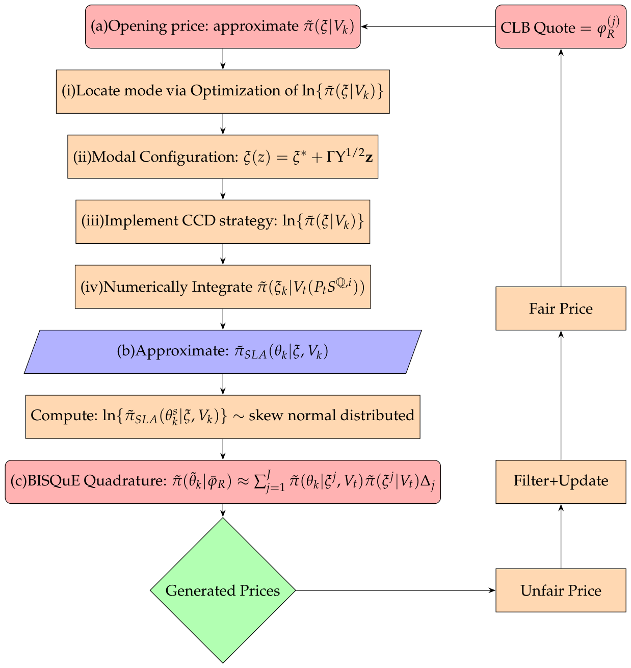
a.

Estimate $\tilde{\pi }\left(\xi \right|V_t\left(P_t{S}^{\mathbb{Q},i}\right))$ the marginal posterior for the hyperparameter $\xi$. The first step requires 4 additional sub-steps such as

(i)

Performing optimization;

(ii)

Modal configuration (finite difference scheme);

(iii)

Central composite design strategy;

(iv)

Numerical integration.

b.

Estimate $\tilde{\pi }\left({\theta }_k\right|\xi ,V_t\left(P_t{S}^{\mathbb{Q},i}\right))$, the posterior marginal for latent parameter $\theta$, by using the simplified Laplace approximation,

c.

Finally, by combining steps (a.) and (b.), we can perform numerical integration on the estimation of posterior marginals of interest for the latent Gaussian field (Sithole et al. 2024):

$$\tilde{\pi }\left({\theta }_k\right|V_t\left(P_t{S}^{\mathbb{Q},i}\right))\approx {\displaystyle \sum _{j=1}^J}\tilde{\pi }\left({\theta }_k\right|{\xi }^j,V_t)\tilde{\pi }\left({\xi }^j\right|V_t){\Delta }_j,$$

(50)

where ${\Delta }_j={\displaystyle \frac{1}{\Sigma \tilde{\pi }\left({\xi }^j\right|V_t)}}$. Thus, we compute the marginal posterior

$\tilde{\pi }\left({\theta }_k\right|V_t\left(P_t{S}^{\mathbb{Q},i}\right))$ by using the Bayesian Inference Sparse-Grid Quadrature Evaluation (BISQuE) quadrature rule.

Next, we present the INLA algorithm that illustrates the flow of three steps and the computation of a fair market price of longevity risk:

a.

Estimating $\tilde{\mathbf{\pi }}\left(\mathbf{\xi }\right|{\mathbf{V}}_{\mathbf{t}}\left({\mathbf{P}}_{\mathbf{t}}{\mathbf{S}}^{\mathbb{Q},\mathbf{i}}\right))$ through exploration:

Exploring $\tilde{\pi }\left(\xi \right|V_t\left(P_t{S}^{\mathbb{Q},i}\right))$ entails an additional four sub-steps as follows:

(i)

Step 1: Using optimization on $ln\left\{\tilde{\pi }\left(\xi \right|V_t\left(P_t{S}^{\mathbb{Q},i}\right))\right\}:=f\left(\xi \right)$ with respect to $\xi$, we can find the location of the distribution mode of $\tilde{\pi }\left(\xi \right|V_t\left(P_t{S}^{\mathbb{Q},i}\right))$.

(ii)

Step 2: At the modal configuration of ${\xi }^{*}$ by utilizing the finite differences scheme, enumerate the Hessian matrix $\mathbf{H}>0$. Consider $\Sigma ={\mathbf{H}}^{-1}$, which is the covariance of $\xi$ and computes its spectral (eigen) decomposition given by ${\mathbf{H}}^{-1}=\Gamma {\rm Y}{\Gamma }^T$, with the aid of a standard variable $\mathbf{z}$, such that

$$\xi \left(\mathbf{z}\right)={\xi }^{*}+\Gamma {{\rm Y}}^{1/2}\mathbf{z}.$$

(51)

(iii)

Step 3: Using $\mathbf{z}$-parameterization, and exploring the approximation of $ln\left\{\tilde{\pi }\left(\xi \right|V_t\left(P_t{S}^{\mathbb{Q},i}\right))\right\}$ in order to find the locus of the entire probability mass. As this approach is computationally demanding, we choose the central composite design (CCD) strategy for the reason of minimizing the computational costs.

(iv)

Estimating $\pi \left({\xi }_k\right|V_t\left(P_t{S}^{\mathbb{Q},i}\right))$: Using numerical integration, we can attain the posterior marginals ${\xi }_k$ precisely from $\tilde{\pi }\left({\xi }_k\right|V_t\left(P_t{S}^{\mathbb{Q},i}\right))$.

b.

Estimate $\mathbf{\pi }\left({\mathbf{\theta }}_{\mathbf{k}}\right|\mathbf{\xi },{\mathbf{V}}_{\mathbf{t}}\left({\mathbf{P}}_{\mathbf{t}}{\mathbf{S}}^{\mathbb{Q},\mathbf{i}}\right))$ by using the simplified Laplace approximation

We employ the SLA based on its ability to converge fast and avoid the other two approaches based on their erroneousness and lack of skewness associated with errors.

(i)

Gaussian approximation: The less computationally demanding estimation is that of the posterior ${\pi }_G\left({\theta }_k\right|\xi ,V_t\left(P_t{S}^{\mathbb{Q},i}\right))$, such that by utilizing recursions based on the asymptotic covariance matrix, the estimation is able to rectify linear constraints.

(ii)

Laplace approximation: The immediate upgrade of the Gaussian approximation converges towards the Laplace approximation given by

$${\tilde{\pi }}_{LA}\left({\theta }_k\right|\xi ,V_t\left(P_t{S}^{\mathbb{Q},i}\right))\propto {\displaystyle \frac{\pi ({\theta }_k,\xi ,V_t)}{{\tilde{\pi }}_{GG}\left({\theta }_{-k}\right|{\theta }_k,{\xi }^k,V_t)}}={\displaystyle \frac{\pi \left(V_t\right|{\theta }_k,{\xi }^k)\pi \left({\theta }_k\right|{\xi }^k)\pi \left({\xi }^k\right)}{{\tilde{\pi }}_{GG}\left({\theta }_{-k}\right|{\theta }_k,{\xi }^k,V_t)}}{|}_{{\theta }_{-k}={\theta }_{-k}^{*}({\theta }_k,\xi )}.$$

(52)

(iii)

Simplified Laplace approximation: We augment ${\tilde{\pi }}_{LA}\left({\theta }_k\right|\xi ,V_t\left(P_t{S}^{\mathbb{Q},i}\right))$, which are represented as a series centered around ${\theta }_k={\mu }_k\left(\xi \right)$, through a derivation of the SLA ${\tilde{\pi }}_{SLA}\left({\theta }_k\right|\xi ,V_t\left(P_t{S}^{\mathbb{Q},i}\right))$. Therefore, this enables for the rectification on the location and the skewness in the Gaussian estimation ${\tilde{\pi }}_G\left({\theta }_k\right|\xi ,V_t\left(P_t{S}^{\mathbb{Q},i}\right))$. Suppose we define a third-order differential equation (ODE) that exists as

$$d_l^{\left(3\right)}({\theta }_k,\xi )={\displaystyle \frac{{\partial }^3}{\partial {\theta }_l^3}}ln\left\{\pi \left(V_l\right|{\theta }_l,\xi )\right)\}{|}_{{\theta }_l={\mathbb{E}}_{{\tilde{\pi }}_G}\left({\theta }_l\right|{\theta }_k)}.$$

(53)

5.2. INLA Belief Inference

In this sub-section, we introduce the idea that rational beliefs can be expressed as weighted numerical probability belief functions. It is crucial that we filter and infer on a belief every time we generate a new posterior using INLA, so as to obtain the best fair market quote for the pensioner’s investment portfolio in our investigation. We, therefore, present properties and axioms that support this notion.

5.2.1. Belief Functions

Suppose we assign plausible statements that define our three parameters that enable us to infer and evaluate beliefs in order to effectively update our posterior distribution every time we compute a new market quote. Let

• $\xi =\{$a hyperparameter containing covariance noise matrices as elements}.
• $\theta =\{$ SA Bond(30Y), Maturity: 28-FEB-2048, price-issue $82.64$, coupon at $8.75$ and survival rate of x aged 65 or older is 0.45 globally}.
• $V_t=\{$a coupon payment at $8.75$ is fair if a pensioner is still alive based on the global survival rate and current longevity bond index is used}.

We define a belief function denoted by $Be(.)$ as a function that aligns statements to a quantity, such that the number lies in the confidence interval $0\le Be(.)\le 1$. Moreover, if $0\le Be(.)<0.95$, is a weak interval of belief, then $0.95\le Be(.)\le 1$ is regarded to be a significantly strong interval of belief.

We further compare the beliefs on the true weight they carry against each other:

a.

$Be\left(\theta \right)>Be\left(\xi \right)$ implies that $\theta$ carries more truth than $\xi$.

b.

$Be\left(\theta \right|V_t)>Be\left(\xi \right|V_t)$ implies that $\theta$ still carries more truth than $\xi$, under the condition that $V_t$ remains true in comparing the two beliefs.

c.

$Be\left(\theta \right|V_t)>Be\left(\theta \right|\xi )$ implies that if we are to predict an outcome on $\xi$, we would rather favour that $V_t$ carries more truth that $\xi$.

5.2.2. Probability Axioms

We now express belief functions from (a.) to (c.) as probability functions governed by axioms as follows (Hoff 2009):

(i.)

$0=\pi (\neg V_t|V_t)\le \pi \left(\xi \right|V_t)\le \pi \left(V_t\right|V_t)=1$.

(ii.)

$\pi (\theta \cup \xi |V_t)=\pi \left(\xi \right|V_t)+\pi \left(\theta \right|V_t)$ if $\theta \cap \xi =\varnothing$.

(iii.)

$\pi (\theta \cap \xi |V_t)=\pi \left(\theta \right|V_t)\pi \left(\xi \right|\theta \cap V_t)$.

Axiom (ii.) is used to generate fair prices, such that $\pi ({\theta }_k,{\xi }_k|V_t)=\pi (\theta \cup \xi |V_t)$ as $\theta \cap \xi =\varnothing$ means that the noise parameter set $\left\{\xi \right\}$ does not intersect with the joint state set $\left\{\theta \right\}$. Therefore, we can update the posterior to a stronger posterior belief which is also a fair market quote denoted as $\pi ({\theta }_{k+1},{\xi }_{k+1}|V_{t+1})$. In other words, if we encounter an unfair (weak belief) price we assign it to axiom (iii.), which acts as a for loop with a belief filtering system, until we effectively remove the noise and then ultimately update it to axiom (ii.).

5.2.3. Belief Filtering and Updating

It is crucial that we tackle the noise that is inherent in the unfair prices by employing Bayes filtering. The belief density function is given by

$$Be\left({\theta }_t\right|V_t)=\pi \left({\theta }_t\right|{\xi }_1,V_2,\dots ,{\xi }_{t-1},V_t),$$

where the Bayes posterior is written as

$$\pi ({\theta }_t,{\xi }_1,V_2,\dots ,{\xi }_{t-1}|V_t)={\displaystyle \frac{1}{z_t}}\pi \left(V_t\right|{\theta }_t,{\xi }_1,V_2,\dots ,{\xi }_{t-1})\pi \left({\theta }_t\right|{\xi }_1,V_2,\dots ,V_{t-1}),$$

where $z_t$ is the normalized evidence. In the likelihood function we discard the parameters ${\xi }_1,V_2,\dots ,{\xi }_{t-1}$ by using the sensor independence property to update the posterior as

$$\pi ({\theta }_t,{\xi }_1,V_2,\dots ,{\xi }_{t-1}|V_t)={\displaystyle \frac{1}{z_t}}\pi \left(V_t\right|{\theta }_t)\pi \left({\theta }_t\right|{\xi }_1,V_2,\dots ,{\xi }_{t-1},{\theta }_{t-1}).$$

Furthermore, in our quantification of the posterior, we consider the total probability of the prior such that we have

$$\pi ({\theta }_t,{\xi }_1,V_2,\dots ,{\xi }_{t-1}|V_t)={\displaystyle \frac{1}{z_t}}\pi \left(V_t\right|{\theta }_t)\int \pi \left({\theta }_t\right|{\xi }_1,V_2,\dots ,{\xi }_{t-1},{\theta }_{t-1})\pi \left({\theta }_t\right|{\xi }_1,V_2,\dots ,{\xi }_{t-1})d{\theta }_{t-1}.$$

The Markovian property discards all the previous history of the likelihood function that is ${\xi }_1,V_2,\dots$, so that we obtain

$$\pi ({\theta }_t,{\xi }_1,V_2,\dots ,{\xi }_{t-1}|V_t)={\displaystyle \frac{1}{z_t}}\pi \left(V_t\right|{\theta }_t)\int \pi \left({\theta }_t\right|{\xi }_{t-1},{\theta }_{t-1})\pi \left({\theta }_t\right|{\xi }_1,V_2,\dots ,{\xi }_{t-1})d{\theta }_{t-1}.$$

Finally, inductively, we have update our belief from the previous time step $t-1$ to t, and we write it as

$$Be\left({\theta }_t\right|V_t)={\displaystyle \frac{1}{z_t}}\pi \left(V_t\right|{\theta }_t)\int \pi \left({\theta }_t\right|{\xi }_{t-1},{\theta }_{t-1})Be\left({\theta }_{t-1}\right|V_{t-1})d{\theta }_{t-1}.$$

5.3. Significance of a Gamma-Distributed Conjugate Prior

Within the Bayesian setup, it is significant to utilize a conjugate prior, as it helps with updating of beliefs and having the prior (such that the prior and the likelihood are in the same closed form) and the posterior in the same distribution. We choose a conjugate prior price that helps generate the projected updated posterior price distribution so that both are in the same distribution.

We present a distribution representation to demonstrate that if the prior has a Gamma distribution, it is conjugate to the Poisson likelihood; then, the posterior is also Gamma-distributed. Suppose that the observed pricing process $V_t\left(P_t{S}^{\mathbb{Q},t}\right)$ is Poisson-distributed and represented as

$$V_t\left(P_t{S}^{\mathbb{Q},t}\right)\sim \mathit{Poisson}({\theta }_k,\xi ),$$

(54)

where this implies that the likelihood thereof has a closed-form given as

$$\pi \left(V_t\left(P_t{S}^{\mathbb{Q},t}\right)\right|\theta ,\xi )={\displaystyle \frac{e^{-\left({\theta }_k\xi \right)}{\left({\theta }_k\xi \right)}^{V_t}}{V_t!}}.$$

(55)

The latent field and hyperparameters are Gamma-distributed such that we have

$${\theta }_k,\xi \sim Gamma(\omega ,ϵ),$$

(56)

where this implies that the prior has a closed-form given as

$${\pi }_0({\theta }_k,\xi )={\displaystyle \frac{{\left(ϵ\right)}^{\omega }{\left({\theta }_k\xi \right)}^{\omega -1}{e}^{-ϵ\left({\theta }_k\xi \right)}}{\Gamma \left(\omega \right)}}\propto {\left({\theta }_k\xi \right)}^{\omega -1}{e}^{-ϵ\left({\theta }_k\xi \right)}.$$

(57)

Furthermore, we expand the Poisson-distributed likelihood to obtain

$$\pi \left(V_t\left(P_t{S}^{\mathbb{Q},t}\right)\right|{\theta }_k,\xi )={\displaystyle \prod _{k=1}^N}{\displaystyle \frac{e^{-{\theta }_k\xi }{\left({\theta }_k\xi \right)}^{V_k}}{V_k!}}={\displaystyle \frac{e^{-N\left({\theta }_k\xi \right)}{\left({\theta }_k\xi \right)}^{V_1+V_2+\dots +V_N}}{{\prod }_{k=1}^N{V}_k!}},$$

(58)

such that

$$\pi \left(V_t\left(P_t{S}^{\mathbb{Q},t}\right)\right|{\theta }_k,\xi )\propto e^{-N\left(\theta \xi \right)}{\left({\theta }_k\xi \right)}^{V_1+V_2+\dots +V_N}=e^{-N\left({\theta }_k\xi \right)}{\left({\theta }_k\xi \right)}^{N{V}_t}.$$

(59)

Using Equations (45), (57) and (59), we obtain a result where the posterior has a normal-Gamma distribution (Gaussian-Gamma distribution) of the same closed-form as the conjugate prior, given as

$$\pi ({\theta }_k,\xi |V_t\left(P_t{S}^{\mathbb{Q},i}\right))\propto \pi \left(V_t\left(P_t{S}^{\mathbb{Q},i}\right)\right|{\theta }_k,\xi ){\pi }_0({\theta }_k,\xi ),$$

$$\propto e^{-N\left({\theta }_k\xi \right)}{\left({\theta }_k\xi \right)}^{N{V}_t}{\left({\theta }_k\xi \right)}^{\omega -1}{e}^{-ϵ\left({\theta }_k\xi \right)},$$

$$\pi ({\theta }_k,\xi |V_t\left(P_t{S}^{\mathbb{Q},i}\right))\propto e^{-(N+ϵ)\left({\theta }_k\xi \right)}{\left({\theta }_k\xi \right)}^{N{V}_t+\omega -1}\sim Gamma(N{V}_t+\omega ,N+ϵ).$$

(60)

In the next section, we present the INLA Incomplete Market Model that allows accurate pricing and hedging of the market price of longevity risk.

6. INLA Incomplete Market Model

We construct a pricing model for the CLBs that employs a risk-neutral method based on the CIR Renshaw–Haberman model to address illiquidity within incomplete markets. The market price of risk is defined as a bounded subset of a Gaussian subspace. This Gaussian subspace in the market is like a CLB index that measures how prices change over a particular term of maturity for a selected portion of the market. Moreover, this implies that the market price of risk is not point-wise identifiable under the setup of the incomplete markets (Kaido and White 2009). The markets with non-zero payouts offer positive prices under the arbitrage-free principle. Consequently, this situation is beneficial for emerging markets and the pensioners, as this implies stringently positive returns and no loss for such markets. Thus, we consider the assumption that our market is arbitrage-free, which is; however, not complete and supported by the following proposition:

Proposition 3 

((Medina and Merino 2003)). If there exists an incomplete market, then the posterior $\pi \left(\theta \right|V_t)$ admits an endless number of arbitrage-free families of price augmentations.

Proposition 4 

((Medina and Merino 2003)). If a market is incomplete, then the sum of all possible arbitrage-free CLB prices (sum of the present value of all cash flow) are a proper set of a Riesz density.

Corollary 1. 

If a market is incomplete, then market admits strigently positive coupon payouts for CLBs for term-to-maturity T that form a convergent monotone decreasing sequence $\pi \left({\theta }_k\right|V_t)\in \mathcal{B}$ (contains all opportunities) that is bounded below, such that the last coupon payout makes the investment fund to be depleted and the principal is paid back to the pensioner.

Proof. 

Suppose that $\pi \left({\theta }_k\right|V_t)=\mathcal{W}$ is a distribution of a bounded sequence of increasing prices; however, due to that, the survival rates decline, causing the posterior coupon payouts to decrease if the interest rate is fixed for a particular bond price sold at face value of $R1000$. Thus, this is a contradiction and $\pi \left({\theta }_k\right|V_t)=\mathcal{G}$ is rather a distribution of a bounded sequence of decreasing prices. Moreover, this is illustrated by that any two priors over time will have the below relation

$$\begin{array}{cc}{\pi }_t\left({\theta }_k\right)\ge {\pi }_{t+1}\left({\theta }_k\right),& {\forall }_{k,t}.\end{array}$$

Consequently, this implies that over an increasing term structure the probability of lower CLBs will increase as we update priors with new data to achieve an updated posterior at each time step. □

Corollary 2. 

The expected price of CLB (a continuous random variable) denoted by $\mathbb{E}\left(\pi \left({\theta }_k\right|V_t)\right)$ on a particular day in an incomplete market that admits endless augmentations of $\pi \left({\theta }_k\right|V_t)$ can be represented by a posterior (probability density function), such that all CLBs $\in \mathcal{S}$ (which contains all hedgeable opportunities) are strictly positive and hedgeable.

Proof. 

Suppose that the expected price of a CLB is represented by $\mathbb{E}\left(\pi \left({\theta }_k\right|V_t)\right)$ is not a continuous random variable; then, this implies that it is a discrete random variable which belongs to a countable set of prices. Based on our initial assumption from Section 3, the posterior $\pi \left({\theta }_k\right|V_t)$ is a continuous probability distribution function. Therefore, if we compute the probability of one discrete random CLB price, the result is zero probability. Subsequently, that is a contradiction as the probability density function is a measure of area under the posterior distribution. Furthermore, the price $V_t$ subject to the incomplete market noise hyperparameter $\xi$, falls between two points c and d, such that it can be represented by the probability density function.

$$\pi (c<V_t\le d)={\int }_c^d{\pi }_{\Xi }\left(\xi \right|V_t)d\xi ,$$

with expected mean of the posterior price given by

$$\mathbb{E}\left(\pi \left({\theta }_k\right|V_t)\right)={\int }_{-\infty }^{\infty }\pi \left({\theta }_k\right|\xi ,V_t)·{\pi }_{\Xi }\left(\xi \right|V_t)d\xi .$$

Thus, a fair CLB convergent price $\mathbb{E}\left(\pi \left({\theta }_k\right|V_t)\right)$ is reached after several re-runs of updating the new prior belief on the Bayesian INLA pricing algorithm. □

This is the same as saying that a market is complete if and only if $n\le N+1$ and there are at minimum n instruments that have linearly independent payouts. Particularly, for our case, we have the market space $\mathcal{S}\subset \mathcal{B}$ (Medina and Merino 2003). Suppose that our market does not permit arbitrage alternatives (opportunities) so as to establish the law of one price such that the pricing function, ${\pi }_0:\mathcal{S}\to \mathbb{R}$, is strongly positive and well-articulated.

Theorem 3 

((Medina and Merino 2003)). Let $\pi :\mathcal{S}\to \mathbb{R}$ be a strongly positive Gaussian functional defined on the Gaussian subspace $\mathcal{S}$ of $L\left(\Omega \right)$. Then, there exists a strongly positive augmentation $\tilde{\pi }:L\left(\Omega \right)\to \mathbb{R}$ to the entire space $L\left(\Omega \right)$. If $\mathcal{S}$ is a proper subspace of $L\left(\Omega \right)$, then there are infinitely countless strongly positive augmentations of π to the entire space $L\left(\Omega \right)$. Hence, the set of strongly positive augmentations is convex.

Proposition 5 

((Medina and Merino 2003)). The scenario for non-redundancy of basic instruments. The market is complete if and only if $N+1=n$.

Proposition 6 

((Medina and Merino 2003)). Suppose that the Law of One Price is sustained, wherein the bid-ask spread is zero. Therefore, the market has no arbitrage opportunities if and only if the pricing functional ${\pi }_0:\mathcal{S}\to \mathbb{R}$ permits a strongly positive augmentation ${\tilde{\pi }}_0:\mathcal{B}\to \mathbb{R}$. Consequently, if the market is incomplete, then there are infinitely countless strongly positive augmentations.

Therefore, we have constructed an incomplete market that permits zero arbitrage opportunities with an underlying martingale measure $\mathbb{Q}$. The First Fundamental Theorem says that we have a no-arbitrage setup if and only if our model has martingale measure $\mathbb{Q}$. The valuation of the risk-free South African government bond is admitted by using the risk-neutral measure and at time-to-maturity t it will be given by $P(0,t):\Omega \to \mathbb{R}$.

Proposition 7 

((Medina and Merino 2003)). Let ${\tilde{\pi }}_0:\mathcal{S}\to \mathbb{R}$ be a stringently positive augmentation of ${\pi }_0$. Moreover, there exists an equivalent martingale measure $\mathbb{Q}$ so that

$$\tilde{\pi }\left({\theta }_k\right)={\pi }^{\mathbb{Q}}\left({\theta }_k\right)=P(i,0)·{\mathbb{E}}^{\mathbb{Q}}\left[{\displaystyle \frac{{\theta }_k}{P(i,1)}}\right],$$

holds for all opportunities where ${\theta }_k\in \mathcal{B}$.

We have a fair price for CLB payout ${\tilde{\pi }}_{fp}\left({\theta }_k\right|V_t)$ if it is hedgeable or, alternatively, if it resides in the set $\mathcal{S}$. Let us consider a non-hedgeable (unfair price) CLB payout ${\pi }_{up}\left({\theta }_k\right|V_t)$. Since the risk-free SA government bond is regarded to be strongly positive, we can write this as

$${\mathcal{D}}_{{\tilde{\pi }}_{fp}\left({\theta }_k\right|V_t)}:=\{{\pi }_{up}\left({\theta }_k\right|V_t)\in \mathcal{S};{\tilde{\pi }}_{fp}\left({\theta }_k\right|V_t)\le {\pi }_{up}\left({\theta }_k\right|V_t)\}\ne \varnothing ,$$

Therefore, every unfair CLB price that is subject to high-risk exposure (also unobservable) ${\pi }_{up}\left(\theta \right|V_t)\in {\mathcal{D}}_{{\tilde{\pi }}_{fp}\left({\theta }_k\right|V_t)}$ is regarded as a $supra$ $hedge$ or a $dominating$ $hedgeable$ payout for ${\tilde{\pi }}_{fp}\left({\theta }_k\right|V_t)$. Now suppose we sell the CLB payout ${\tilde{\pi }}_{fp}\left({\theta }_k\right|V_t)$ for the fair price of ${\pi }_0\left({\theta }_k\right|V_t)$, with ${\pi }_{up}\left({\theta }_k\right|V_t)\in {\mathcal{D}}_{{\pi }_{up}\left({\theta }_k\right|V_t)}$; this will allow us to implement a hedging strategy for the unfair price ${\pi }_{up}\left({\theta }_k\right|V_t)$. Due to the inequality ${\tilde{\pi }}_{fp}\left({\theta }_k\right|V_t)\le {\pi }_{up}\left({\theta }_k\right|V_t)$ the payout that was accumulated from the hedge of ${\pi }_{up}\left({\theta }_k\right|V_t)$ will always be sufficient to sustain the fair quote of ${\tilde{\pi }}_{fp}\left({\theta }_k\right|V_t)$. The argument of interest is that, given that there is no fair price in the market space such that ${\tilde{\pi }}_{fp}\left({\theta }_k\right|V_t)\notin \mathcal{S}$, is it probable to determine an opportunity in the market where ${\pi }_{up}\left({\theta }_k\right|V_t)\in \mathcal{S}$ agrees with the condition ${\tilde{\pi }}_{fp}\left(\theta \right|V_t)\le {\pi }_{up}\left({\theta }_k\right|V_t)\}$ under the minimum hedgeable cost? If such a scenario is feasible, then it is natural to maintain the CLB price ${\tilde{\pi }}_{fp}\left({\theta }_k\right|V_t)$ for non-hedgeable opportunities, since this cost is minimal for a dominating hedgeable opportunity. Additionally, by applying the Girsanov Theorem, we utilize the Girsanov kernel process $h_t$. Here, the market price of longevity risk ${\phi }_R$ is derived from the stochastic differential Equation (13) such that $h_t=\left|{\phi }_R\right|$; then,

$${\phi }_R={\displaystyle \frac{{\alpha }_{\lambda }-{\theta }_k}{{\sigma }_{\lambda }{a}^r(t,T_D)b_r}},$$

so that we can generate a risk-neutral probability measure for the longevity risk premium denoted by $\mathbb{Q}\left({\phi }_R\right)$, with ${\phi }_R={\left[{\phi }_1{\phi }_2\right]}^T$ to obtain

$${\tilde{\theta }}_{k+1}={\tilde{\theta }}_k+\tilde{\rho }+C\tilde{U},$$

where the Cholesky decomposition of $\Sigma$ is denoted as C. Also, $\tilde{U}={\phi }_R+U$ with $\tilde{U}\sim N(0,{\mathbf{I}}_2)$ under the risk-neutral probability measure $\mathbb{Q}\left({\phi }_R\right)$ and $\tilde{\rho }=A-C{\phi }_R$ (Leung et al. 2018). We mathematically assemble the mortality index as

$$\tilde{S}(t,T)={\mathbb{E}}^{{\mathbb{P}}_2\left({\phi }_1\right)}\left[{\displaystyle \prod _{l=1}^t}(1-{\tilde{m}}_{x_1+l,t_0+l})\right],$$

where ${\tilde{m}}_{x,t}$ is the crude death rate that is taken from Equations (19) and (21), and we use ${\tilde{\theta }}_k$, the joint state process that is presented in Equation (25) (Cairns et al. 2006).

With the intelligent risk-neutral pricing method, we shall be able to generate the market price of longevity risk ${\phi }_R$ by utilizing the optimized minima difference equation between the risk-neutral price and the inception price of the South African Government 30Y bond, given by

$${\widehat{\phi }}_R=arg\underset{{\phi }_R}{min}\left({\displaystyle \sum _{t=1}^T}\underset{risk-neutral-price}{\underbrace{P(t,T)exp\left\{\delta (T-t)\right\}\tilde{S}(t,T)}}-\underset{Inception-price}{\underbrace{P(0,t)exp\left\{\delta t\right\}{\mathbb{E}}^{\mathbb{P}}\left[S(0,t)\right]}}\right).$$

(61)

Consequently, there exists an infinite number of candidates for ${\phi }_R$, with the presumption that South African Government 30Y bond price is accessible. In this paper, we are interested in the case where ${\phi }_{\mathbf{R}}=\{{\phi }_1=\mathrm{interest}\mathrm{rate}\mathrm{risk}\mathrm{premium},{\phi }_2=\mathrm{mortality}\mathrm{risk}\mathrm{premium}\}$, since our pricing model relies on the posterior (Bayesian state-space representation) given as

$$\pi \left({\theta }_k\right|{\mathbf{V}}_k)=\mathcal{N}\left({\theta }_k\right|{\widehat{\theta }}_k,{\Sigma }_{k|k}),$$

(62)

which is built within the Bayesian INLA framework. In the study by Leung et al., the MCMC sampling technique is used to quantify the posterior distribution market price (Leung et al. 2018), and we improve the model with the faster INLA approximation technique that handles the curse of dimensionality efficiently. Therefore, every one of these sequentially updated jth approximations of the latent parameters represents the possible joint state process and can generate a risk-neutral state prior distribution of $\pi \left(\tilde{\theta }\right)$ given as

$$\pi \left({\tilde{\theta }}_{k+1}^{\left(i\right)}\right)=\pi ({\tilde{\theta }}_k^{\left(i\right)}+{\tilde{\rho }}^{\left(i\right)}+C^{\left(i\right)}{\tilde{U}}^{\left(i\right)}),$$

where ${\tilde{\rho }}^{\left(i\right)}=A^{\left(i\right)}-C^{\left(i\right)}{\phi }_R^{\left(i\right)}$. Hence, an INLA-based approximation of the posterior distribution given by $\tilde{\pi }\left(\tilde{\theta }\right|{\widehat{\phi }}_R)={\sum }_{\ell =1}^{k_i}\tilde{\pi }({\theta }_k,{\xi }^{(i,\ell )}|V_t){\tilde{w}}^{(i,\ell )}$ can be utilized to propagate the market price of longevity risk${\phi }_R^{\left(i\right)}$ across latent parameters that are generally dependent upon interest rate dynamics (driven by inflation risk), bond spread dynamics (driven by illiquidity risk) and mortality tendencies (Hewitt and Hoeting 2019).

7. Analysis and Results

In this section1, we look at the INLA pricing process flow diagram, compare INLA against the MCMC, and utilize the longevity Greeks to analyze the longevity risk exposure of the cohort aged 65 in 2006 and study the liabilities incurred until 2018 (age 77). Here, the survivors have surpassed the life expectancies for the term horizon interval, 2006 to 2018. Figure 1 illustrates the INLA pricing system which removes noisy unfairly priced CLB, subsequently filtering and updating them as fair CLB prices for the incomplete longevity bonds’ market. In Figure 2 and

Table 1. CLB prices using 30Y South African Government Bonds’ (SA GB) yield data from the South African Debt Market and survival rates extracted from Stats SA data mid-year reports from 2006 until 2018 (Government Employees Pension Fund 2019, 2023; Statistics South Africa 2018).

Maturity	Cohort	Yield 30Y	Spread	30Y	$\widehat{{\mathit{\phi }}_{\mathit{R}}}$:CLB	Coupons
Date	1941$:\mathit{S}\left(\mathit{t}\right)$	SA GB	$exp\left\{\mathit{\delta }\mathit{t}\right\}$	GB Prices	in Rands	p.a.
14 November 2006	0.945	7.165	1.00225	1353.99	1282.40	282.40
27 July 2007	0.944	8.01	1.00451	1384.77	1313.12	313.12
29 July 2008	0.943	8.985	1.00677	1388.39	1318.12	318.12
5 August 2009	0.942	8.57	1.00904	1462.89	1390.50	390.50
27 July 2010	0.942	8.615	1.01131	1506.11	1434.81	434.81
27 May 2011	0.939	8.69	1.01359	1542.33	1467.93	467.93
31 August 2012	0.937	8.145	1.01587	1631.63	1553.11	553.11
17 September 2013	0.926	9.04	1.01816	1581.99	1491.53	491.53
4 February 2014	0.93	9.345	1.02045	1581.01	1500.42	500.42
6 October 2015	0.926	8.9	1.02275	1654.77	1567.18	567.18
22 March 2016	0.923	10.065	1.02505	1551.89	1468.29	468.29
7 May 2017	0.922	9.725	1.02736	1607.09	1522.29	522.29
14 September 2018	0.916	10.23	1.02968	1566.65	1477.65	477.65

, the INLA posteriors are compared with the traditional MCMC posteriors. It is well noticeable that the noise variance associated with the hyperparameter ${\xi }_k$ is quite low around $0.0315$ and the posterior CLB mean ${\mu }_{CLB}$ associated with the latent parameter ${\theta }_k$ has a mean valued at approximately $1444.77$. Both plots illustrate that the methods have almost identical approximations for the posteriors. However, INLA is more consistent, parsimonious and reliable as seen in it is smoothness and symmetry. Figure 3: ${\Delta }_{\mathbf{x}},\mathbf{t}={\sum }_{\mathbf{s}=\mathbf{1}}^{\mathbf{13}}\left[{(\mathbf{1}+\mathbf{YTM})}^{-\mathbf{s}}\mathbf{LongPay}·(\mathbf{sensitivity}·\mathbf{delta})\right]$, which represents the longevity delta model that quantifies first-order sensitivity of CLB with respect to latent parameter ${\theta }_k$. Furthermore, the longevity delta gives a reflection on the exposure to longevity risk, while the longevity gamma model ${\Gamma }_{\mathbf{x}},\mathbf{t}={\sum }_{\mathbf{s}=\mathbf{1}}^{\mathbf{13}}\left[{(\mathbf{1}+\mathbf{YTM})}^{-\mathbf{s}}\mathbf{LongPay}·(\mathbf{sensitivity}·\mathbf{gamma})\right]$ measures the second-order sensitivity of CLB with respect to the latent parameter ${\theta }_k$. As a second-order equation, it reflects that the longevity risk exposure is concave down, with a local maximum at zero. Longevity vega ${\nu }_{\mathbf{x},\mathbf{t}}={\sum }_{\mathbf{s}=\mathbf{1}}^{\mathbf{13}}\left[{(\mathbf{1}+\mathbf{YTM})}^{-\mathbf{s}}\mathbf{LongPay}·(\mathbf{sensitivity}·\mathbf{vega})\right]$ computes the first-order sensitivity of CLB with respect to the conditional volatility $h_0$, (Zhou and Li 2017). Thus, the longevity vega quantifies the sensitivity to uncertainty in mortality projections attributed to the prolonged time effect of longevity payouts. Figure 3 shows that all the longevity Greeks are negative and tend asymptotically towards zero as they become less negative as ${\mathbf{t}}_{\mathbf{f}}$ increases. In addition, as ${\mathbf{t}}_{\mathbf{f}}$ increases, we have a situation where the insurance firm has an increased time horizon (time-to-maturity) which then leads to exacerbated payouts as a result of individuals outliving the cohort (Zhou 2019). As the insurer’s time horizon ${\mathbf{t}}_{\mathbf{f}}$ expands, the hedging strategy is to activate the reinsurance mechanism through the use of q-forwards (or longevity swaps) that carry higher notional reserves to match the growing uncertainty in mortality improvements (Zhou 2019). Here, a longer time horizon implies an increase in exposure to uncertainty in mortality forecasts, justified by less negative longevity Greek values. Moreover, we also observe the inequality $\left({\Delta }_{\mathbf{x},\mathbf{t}}<{\Gamma }_{\mathbf{x},\mathbf{t}}<{\nu }_{\mathbf{x},\mathbf{t}}\right)$, as shown in Figure 3, and there is definitely exacerbated longevity risk exposure in the age interval $[\mathbf{65},\mathbf{68}]$, due to a mispredicted surge of outliving pensioners, thus resulting in an increase in longevity payouts. Thus, instead of employing a single homogeneous index, the concentration of increased sensitivity in the interval $[\mathbf{65},\mathbf{68}]$ may be hedged by focusing q-forwards on that particular cohort band. A dynamic hedging strategy that offsets the delta, gamma, and vega sensitivities over time is likely to be effective in attenuating residual longevity risk, particularly in the context of regime-switching mortality volatility and mortality improvement reserves (MIRs), which are often extended on a year-to-year basis by the Government Employees Pension Fund (GEPF). This means that the hedging framework must be periodically recalibrated—by adjusting q-forward or longevity-swap notional levels and cohort targeting—to match the updated MIRs and the evolving latent time effect of mortality.

Table 2. An aspect comparison between the traditional MCMC and Bayesian INLA. Here, MCMC relies on iterative sampling via the joint posterior, while the INLA computes the marginal posteriors deterministically via the nested Laplace approximations on latent GMRFs.

Aspect	Trad. MCMC	Bayesian INLA	Quant. Evidence
Methodology	Gibbs sampling,	Deterministic nested,	MCMC: 100k iters,
	asymptotically exact.	on latent GMRF.	(20 min); INLA 4 min (Taylor and Diggle 2014).
Convergence	Slow 10 k–250 k iters.	Instant marginals,	MCMC: 42k iters avg,
		direct marginals.	INLA: <1 s ${10}^4$ obs (De Smedt et al. 2015).
Runtime	3–250+ min,	1–30 s, 42–100× faster.	INLA 42× faster.
	spatial models.
Comp. Cost	High autocorr,	Sparse Cholesky,	INLA 39 min,
	(IA = 0.8–0.95).	$\mathcal{O}(n^{2}logn)$.	MCMC 20 min.
Dimensionality	Mixing$\propto exp(-d)$,	GMRF scales ${10}^5$–${10}^6$,	MCMC fails ${10}^4+$,
	fails $>{10}^4$ obs	parameters.	INLA handles ${10}^6+$.
Scalability	${10}^3$–${10}^4$ obs max.	${10}^6+$ obs,	INLA viable,
		SPDE/GMRF.	national data.
Accuracy	Gold standard,	85–91% CI overlap,	Identical simulation,
	exact limit.	w/MCMC.	except rare events (Darkwah 2022).
Math Expense	${10}^{10}$ likelihood,	${10}^3$–${10}^4$ ops total	Orders of magnitude,
	evals/iter.		cheaper.
Flexibility	Any model,	Latent Gaussian,	INLA = screening,
	non-Gaussian.	(GLMM/spatial).	MCMC = validation (Padmanabhan 2022).

compares traditional MCMC and Bayesian INLA across nine computational dimensions. INLA consistently outperforms MCMC in runtime ($42\times$ faster), scalability (${10}^6+$ observations via SPDE/GMRF), and computational cost (sparse Cholesky; $\mathcal{O}(n^{2}logn)$), while maintaining 85–$91\%$ CI overlap with MCMC. Although MCMC remains the gold standard for exact inference and non-Gaussian flexibility, INLA is the preferred estimation framework for high-dimensional latent Gaussian models, with MCMC reserved for validation.

In

Table 3. Longevity risk metrics for the South African market, comprising annual observations of mortality improvement rates (MIRs), survival rates, life expectancy, longevity payouts, and longevity Greeks (longevity delta ${\Delta }_{xt}$, longevity gamma ${\Gamma }_{x,t}$, and longevity vega ${\nu }_{x,t}$) across selected age cohorts.

Year (${\mathbf{t}}_{\mathit{f}}$)	Age	AvLifeExp	${\mathit{S}}^{\mathbb{Q},\mathit{i}}\left(\mathit{t}\right)$	MIR	LongPay	${\mathbf{\Delta }}_{\mathit{x},\mathit{t}}$	${\mathbf{\Gamma }}_{\mathit{x},\mathit{t}}$	${\mathit{\nu }}_{\mathit{x},\mathit{t}}$
2006	65	54.1	0.945	11.387	7.743 (est.)	−1.90 $\times {10}^1$	−9.48 $\times {10}^0$	−4.47 $\times {10}^1$
2007	66	54.9	0.944	11.387	9.188 (est.)	−2.26 $\times {10}^0$	−1.13 $\times {10}^0$	−5.66 $\times {10}^{-1}$
2008	67	56	0.9437	15.638	10.634 (est.)	−2.14 $\times {10}^{-1}$	−1.07 $\times {10}^{-1}$	−5.34 $\times {10}^{-2}$
2009	68	57.4	0.942	15.638	11.691 (est.)	−2.79 $\times {10}^{-2}$	−1.39 $\times {10}^{-2}$	−6.97 $\times {10}^{-3}$
2010	69	58.9	0.942	18.748	12.749 (est.)	−3.10 $\times {10}^{-3}$	−1.55 $\times {10}^{-3}$	−7.76 $\times {10}^{-4}$
2011	70	59.9	0.939	18.748	15.428 (est.)	−3.73 $\times {10}^{-4}$	−1.86 $\times {10}^{-4}$	−9.32 $\times {10}^{-5}$
2012	71	61.2	0.937	26.628	18.107 (est.)	−6.77 $\times {10}^{-5}$	−3.39 $\times {10}^{-5}$	−1.69 $\times {10}^{-5}$
2013	72	61.8	0.926	26.628	20.585 (est.)	−3.99 $\times {10}^{-6}$	−1.99 $\times {10}^{-6}$	−9.97 $\times {10}^{-7}$
2014	73	62.5	0.93	33.918	23.064 (est.)	−3.40 $\times {10}^{-7}$	−1.70 $\times {10}^{-7}$	−8.50 $\times {10}^{-8}$
2015	74	62.8	0.926	33.918	25.587 (est.)	−5.66 $\times {10}^{-8}$	−2.83 $\times {10}^{-8}$	−1.41 $\times {10}^{-8}$
2016	75	63.2	0.923	41.340	28.111 (est.)	−1.85 $\times {10}^{-9}$	−9.23 $\times {10}^{-10}$	−4.62 $\times {10}^{-10}$
2017	76	63.9	0.922	41.340	30.476 (est.)	−2.63 $\times {10}^{-10}$	−1.32 $\times {10}^{-10}$	−6.58 $\times {10}^{-11}$
2018	77	$\mathbf{64}.\mathbf{2}$	0.916	48.259	32.841	−1.45 $\times {10}^{-13}$	−7.27 $\times {10}^{-12}$	−3.63 $\times {10}^{-12}$

, the life expectancies and survival rates are extracted from Stats SA data mid-year reports from 2006 to 2018 (Government Employees Pension Fund 2019, 2023; Statistics South Africa 2018). The MIR column represents the mortality improvement reserves (MIRs) in billion rand taken from the GEPF reports from 2006 until 2018. The longevity payouts (LongPay) from 2006 to 2017 are not reported in the GEPF reports. Thus, we estimate them using the 2018 Alexander Forbes valuation that sets a benchmark, wherein the R32 841 million (LongPay) is set as an allowance for active members (future pensioners) outliving the cohort. Moreover, in this study, we assume that the R32 841 million represents the longevity payouts for 2018 (Alexander Forbes Financial Services 2018). Moreover, reflecting a present value with an excess of longevity payouts rated at $2.5$ years younger than the actual age.

Table 4. Comprehensive descriptive statistics.

Statistic	St	30Yields	Spread	CLBs	MIR	LongPay	Age	AvLifeEx	Delta	Gamma	Vega
Mean	0.93346	8.8835	1.0159	1445.2	26,429	18,939	71	60.062	−0.05972	−0.02986	−0.01493
SE	0.00276	0.23527	0.00247	25.691	3431.5	2358.4	1.0801	0.9694	0.05299	0.02649	0.01325
Median	0.937	8.9	1.0159	1468.3	26,628	18,107	71	61.2	−2.07 $\times {10}^{-6}$	−1.03 $\times {10}^{-6}$	−5.17 $\times {10}^{-7}$
Mode	0.926				11,387
Std	0.00997	0.84826	0.00890	92.63	12,372	8503.4	3.8944	3.4954	0.19108	0.09554	0.04777
Variance	9.94 $\times {10}^{-5}$	0.71955	7.92 $\times {10}^{-5}$	8580.2	1.53 $\times {10}^8$	7.23 $\times {10}^7$	15.167	12.218	0.03651	0.00913	0.00228
Kurtosis	−1.4366	0.17394	−1.1998	−0.773	−1.1691	−1.3353	−1.2	−1.15	12.5899	12.5899	12.5899
Skewness	−0.3787	−0.2277	0.01127	−0.616	0.3977	0.288	−4.27 $\times {10}^{-17}$	−0.546	−3.5319	−3.5319	−3.5319
Range	0.029	3.065	0.02743	284.78	36,872	25,098	12	10.1	0.69173	0.34587	0.17293
Min	0.916	7.165	1.0023	1282.4	11,387	7743	65	54.1	−0.69173	−0.34587	−0.17293
Max	0.945	10.23	1.0297	1567.2	48,259	32,841	77	64.2	−2.11 $\times {10}^{-13}$	−1.06 $\times {10}^{-13}$	−5.29 $\times {10}^{-14}$
Sum	12.135	115.48	13.207	18,787	343,577	246,204	923	780.8	−0.77632	−0.38816	−0.19408
Count	13	13	13	13	13	13	13	13	13	13	13
CI (95%)	0.00603	0.5126	0.00538	55.976	7476.5	5138.5	2.3534	2.1122	0.11547	0.057734	0.02887

reveals that South Africa’s incomplete and emerging longevity risk market exhibits significant variability and non-normal distributions across paramount risk metrics: the MIR averages $R26.429$ billion (std $R12.372$ billion; CV $\approx 47\%$), LongPay averages $R18.939$ billion (std $R8.503$ billion; CV $\approx 45\%$), and AvLifeEx averages $60.062$ years (std $3.495$; CV $\approx 6\%$). While positive skewness in MIR (0.398) and LongPay (0.288) suggests right-leaning pull toward high values, AvLifeEx has a negative skewness (−0.546), which suggests a left-tail lag from shorter life expectancies in cohorts. Both the MIR and LongPay have negative kurtosis, indicating platykurtic tails with fewer extreme outliers than normal, thus attenuating sudden downward shocks but signalling consistent moderate spreads. The LongPay’s positive skewness and high CV indicate that payouts will most probably increase under the stochastic trends prevailing in the market, with a mean of $R8.503Bn$, which suggests frequent jumps over the $R20–R27$ billion range. Given that each $+1$ year shift causes an increase in cohort outliving by 15–20% per MIR-linked reserves. Moreover, incorporating AvLifeEx (3.5 years) via the AJD model projects a 5–10% annual LongPay boost if skewness persists. The platykurtic (flat) shaped distribution widens the tails, thereby projecting median longevity payouts stabilizing at $R19Bn$, with a 75th percentile reaching $R24Bn$ during periods of medical advancements.

8. Conclusions

The main objective of this work was to construct a Bayesian pricing model for the coupon longevity bonds’ market. We illustrated that mortality rates and interest rates should be observed independently. These two rates are captured by a discretized CIR-AJD-Renshaw–Haberman state-space model that is aligned with the Bayesian INLA that has an underlying LGM and GMRF frameworks. We proved that our Bayesian state-space model estimates the posterior Gaussian density. The supremacy of the INLA algorithm with belief inference is illustrated and compared against the MCMC, which has a low efficacy in aspects such as methodology, convergence, runtime, dimensionality, computational cost, dimensionality, scalability, accuracy, math expense, and flexibility. Both the MCMC and INLA posterior models were trained on South African government bond yield data, survival rates taken from Stats SA, and GEPF data. We used longevity Greeks as a longevity risk exposure analysis tool to help practitioners, decision makers, and fund managers to assess the hedging strategies of longevity risk and to mitigate uncertainty associated with surging demand for mortality improvement reserves that curb the prolonged longevity payouts. Findings show a negative kurtosis in average life expectancies, implying a tailed distribution that signals the existence of outliers that need to be addressed by practitioners to hedge longevity risk associated with increasing longevity payouts. The longevity payouts exhibit a positive skewness and high CV, indicating that they have a strong likelihood of increasing over time under the stochastic trends prevailing in the market, with a manageable mean, which suggests frequent jumps over the $R20–R27$ billion range.

References

- Alexander Forbes Financial Services. 2018. Government Employees Pension Fund Statutory Actuarial Valuation as at 31 March 2018; Pretoria: Government Employees Pension Fund. Available online: https://www.gepf.co.za/wp-content/uploads/2025/02/GEPF_Statutory_Actuarial_Valution_31_March_2018.pdf (accessed on 30 November 2025).
- Arasaratnam, Ienkaran, and Simon Haykin. 2009. Cubature Kalman filters. IEEE Transactions on Automatic Control 54: 1254–69. [Google Scholar] [CrossRef]
- Bhattacharya, Arnab, and Simon Wilson. 2015. Sequential Bayesian inference for dynamic state space model parameters. In Current Trends in Bayesian Methodology with Applications. Boca Raton: CRC, pp. 123–33. [Google Scholar]
- Blake, David, and Andrew J. G. Cairns. 2025. Longevity risk and capital markets: The 2023–2024 update. In Geneva Papers on Risk and Insurance: Issues and Practice. Berlin and Heidelberg: Springer. [Google Scholar] [CrossRef]
- Blake, David, Andrew Cairns, and Kevin Dowd. 2006. Living with mortality: Longevity bonds and other mortality-linked securities. British Actuarial Journal 12: 153–97. [Google Scholar] [CrossRef]
- Bravo, Jorge Miguel. 2022. Pricing participating longevity-linked life annuities: A Bayesian Model Ensemble approach. European Actuarial Journal 12: 125–59. [Google Scholar] [PubMed]
- Cairns, Andrew J. G., David Blake, and Kevin Dowd. 2006. A two-factor model for stochastic mortality with parameter uncertainty: Theory and calibration. Journal of Risk and Insurance 73: 687–718. [Google Scholar] [CrossRef]
- Carter, Chris K., and Robert Kohn. 1994. On Gibbs sampling for state-space models. Biometrika 81: 541–53. [Google Scholar] [CrossRef]
- Chen, Hua, and Samuel H. Cox. 2009. Modeling mortality with jumps: Applications to mortality securitization. Journal of Risk and Insurance 76: 727–51. [Google Scholar] [CrossRef]
- Darkwah, J. 2022. Bayesian inference for simple and generalized linear models: Comparing INLA and McMC. In Advances in Phytochemistry, Textile and Renewable Energy Research for Industrial Growth. Boca Raton: CRC Press, pp. 62–67. [Google Scholar]
- De Smedt, Tom, Koen Simons, An Van Nieuwenhuyse, and Geert Molenberghs. 2015. Comparing MCMC and INLA for disease mapping with Bayesian hierarchical models. Archives of Public Health 73: O2. [Google Scholar] [CrossRef]
- Fong, Edwin, Chris Holmes, and Stephen G. Walker. 2023. Martingale posterior distributions. Journal of the Royal Statistical Society Series B: Statistical Methodology 85: 1357–91. [Google Scholar] [CrossRef]
- Fushimi, Takahiro, and A. Kogure. 2014. A Bayesian approach to longevity derivative pricing under stochastic interest rates with a two-factor Lee-Carter model. In ARIA 2014 Annual Meeting. University Park: Citeseer, vol. 4. [Google Scholar]
- Government Employees Pension Fund. 2019. Government Employees Pension Fund 2018/2019 Annual Report. Submitted to the Speaker of Parliament. Available online: https://www.gepf.co.za/wp-content/uploads/2025/01/GEPF-Annual-Report-Approved-20191129.pdf (accessed on 30 November 2025).
- Government Employees Pension Fund. 2023. Government Employees Pension Fund—Annual Report 2022/23. Submitted to the Speaker of Parliament. Available online: https://www.gepf.co.za/wp-content/uploads/2025/01/GEPF-Annual-Report-2023-Final.pdf (accessed on 30 November 2025).
- Guo, Yiping, and Johnny Siu-Hang Li. 2025. Fast estimation of the Renshaw-Haberman model and its variants. European Actuarial Journal 15: 633–66. [Google Scholar] [CrossRef]
- Hewitt, Joshua, and Jennifer A. Hoeting. 2019. Approximate Bayesian inference via sparse grid quadrature evaluation for hierarchical models. arXiv arXiv:1904.07270. [Google Scholar]
- Hoff, Peter D. 2009. A First Course in Bayesian Statistical Methods. Berlin and Heidelberg: Springer, vol. 580. [Google Scholar]
- Ikpe, Dennis, Yethu Sithole, and Samuel Asante Gyamerah. 2022. On a consistent state-space bond markets model for pricing long-maturity bonds. International Journal of Financial Engineering 9: 2250024. [Google Scholar]
- Kaido, Hiroaki, and Halbert White. 2009. Inference on risk-neutral measures for incomplete markets. Journal of Financial Econometrics 7: 199–246. [Google Scholar] [CrossRef]
- Lemaire, Vincent, Michéle Thieullen, and Nicolas Thomas. 2020. Thinning and multilevel Monte Carlo methods for piecewise deterministic (Markov) processes with an application to a stochastic Morris–Lecar model. Advances in Applied Probability 52: 138–72. [Google Scholar] [CrossRef]
- Leung, Melvern, Man Chung Fung, and Colin O’hare. 2018. A comparative study of pricing approaches for longevity instruments. Insurance: Mathematics and Economics 82: 95–116. [Google Scholar] [CrossRef]
- Liu, Xiaoming, Rogemar Mamon, and Huan Gao. 2014. A generalized pricing framework addressing correlated mortality and interest risks: A change of probability measure approach. Stochastics: An International Journal of Probability and Stochastic Processes 86: 594–608. [Google Scholar] [CrossRef]
- Martin, Gael M., Brendan P. M. McCabe, David T. Frazier, Worapree Maneesoonthorn, and Christian P. Robert. 2019. Auxiliary likelihood-based approximate Bayesian computation in state-space models. Journal of Computational and Graphical Statistics 28: 508–22. [Google Scholar] [CrossRef]
- Martino, Sara, and Andrea Riebler. 2019. Integrated nested Laplace approximations (INLA). arXiv arXiv:1907.01248. [Google Scholar]
- Martino, Sara, and Havard Rue. 2009. Implementing Approximate Bayesian Inference Using Integrated Nested Laplace Approximation: A Manual for the Inla Program. Trondheim: Department of Mathematical Sciences, NTNU. [Google Scholar]
- Medina, Pablo Koch, and Sandro Merino. 2003. Mathematical Finance and Probability. Berlin and Heidelberg: Springer. [Google Scholar]
- Menoncin, Francesco. 2008. The role of longevity bonds in optimal portfolios. Insurance: Mathematics and Economics 42: 343–58. [Google Scholar] [CrossRef]
- Olivieri, Annamaria, and Ermanno Pitacco. 2008. Assessing the cost of capital for longevity risk. Insurance: Mathematics and Economics 42: 1013–21. [Google Scholar] [CrossRef]
- Padmanabhan, Krishna. 2022. MCMC vs. INLA in Bayesian adaptive clinical trial designs: Comparing simulation-based and approximate Bayesian inference. Paper presented at BAYES2022: Bayesian Biostatistics Conference, Bethesda, MD, USA, October 12–14; Available online: https://cytel.com/perspectives/bayesian-adaptive-clinical-trial-designs-inla-vs-mcmc/ (accessed on 4 June 2026).
- Renshaw, A. E., and Steven Haberman. 2006. A cohort-based extension to the Lee–Carter model for mortality reduction factors. Insurance: Mathematics and Economics 38: 556–70. [Google Scholar] [CrossRef]
- Rue, Håvard, Sara Martino, and Nicolas Chopin. 2009. Approximate Bayesian inference for latent Gaussian models by using integrated nested Laplace approximations. Journal of the Royal Statistical Society: Series B (Statistical Methodology) 71: 319–92. [Google Scholar] [CrossRef]
- Ruiz-Cárdenas, Ramiro, Elias T. Krainski, and Håvard Rue. 2010. Fitting Dynamic Models Using Integrated Nested Laplace Approximations-INLA. Available online: https://www.math.ntnu.no/preprint/statistics/2010/S12-2010.pdf (accessed on 30 November 2025).
- Sahin, Şule, and Shaun Levitan. 2021. A stochastic investment model for actuarial use in South Africa. South African Actuarial Journal 20: 49–79. [Google Scholar] [CrossRef]
- Särkkä, Simo. 2013. Bayesian Filtering and Smoothing. Cambridge, UK: Cambridge University Press, vol. 3. [Google Scholar]
- Shen, Weiwei, and Yan Zhang. 2025. Strong convergence of the Euler-Maruyama method for the stochastic volatility jump-diffusion model and financial applications. AIMS Mathematics 10: 12032–54. [Google Scholar] [CrossRef]
- Shenoy, Prakash P., and Glenn Shafer. 1990. Axioms for probability and belief-function propagation. In Machine Intelligence and Pattern Recognition. Amsterdam: Elsevier, vol. 9, pp. 169–198. [Google Scholar]
- Shi, Jianjie, Yunyun Wang, and Dan Zhu. 2025. A Bayesian Additive Tree Approach to Mortality Forecasting and Nowcasting. SSRN Working Paper 6489138. Available online: https://ssrn.com/abstract=6489138 (accessed on 4 June 2026).
- Sithole, Yethu, Eeva Maria Rapoo, and Samuel Asante Gyamerah. 2024. Assessing the impact of geopolitical risk on longevity bond pricing: Insights from Bayesian multivariate regression. Journal of Statistical Theory and Applications 24: 1–41. [Google Scholar] [CrossRef]
- Statistics South Africa. 2018. Mid-Year Population Estimates, 2018; Statistical Release P0302. Pretoria: Statistics South Africa. Available online: https://www.statssa.gov.za/publications/P0302/P03022018.pdf (accessed on 30 November 2025).
- Takadong, Thibaut Zafack. 2009. Pricing Models for Inflation Linked Derivatives in an Illiquid Market. Unpublished Master’s thesis, University of the Witwatersrand, Johannesburg, South Africa. [Google Scholar]
- Taylor, Benjamin M., and Peter J. Diggle. 2014. INLA or MCMC? A tutorial and comparative evaluation for spatial prediction in log-Gaussian Cox processes. Journal of Statistical Computation and Simulation 84: 2266–84. [Google Scholar]
- Tierney, Luke, and Joseph B. Kadane. 1986. Accurate approximations for posterior moments and marginal densities. Journal of the American Statistical Association 81: 82–86. [Google Scholar] [CrossRef]
- Xu, Jingtong, Xu Chen, and Yuying Yang. 2024. Pricing longevity bond with affine-jump-diffusion multi-cohort mortality model. Journal of Computational and Applied Mathematics 446: 115800. [Google Scholar] [CrossRef]
- Zeddouk, Fadoua, and Pierre Devolder. 2019. Pricing of longevity derivatives and cost of capital. Risks 7: 41. [Google Scholar] [CrossRef]
- Zhou, Kenneth Qian. 2019. Longevity Risk Management: Models and Hedging Strategies. Doctoral dissertation, University of Waterloo, Waterloo, ON, Canada. Available online: https://uwspace.uwaterloo.ca/handle/10012/14530 (accessed on 13 April 2026).
- Zhou, Kenneth Qian, and Johnny Siu-Hang Li. 2017. Longevity Greeks: What should insurers and capital market investors know about? Paper presented at the Living to 100 Symposium, Orlando, FL, USA, January 4–6. [Google Scholar]