Longevity Option and Longevity Swap De-Risking Strategies Under Frailty-Based Mortality Models

Abstract

In this research, we develop longevity option and longevity swap de-risking strategies based on a frailty-based mortality model in order to obtain more effective longevity risk transfer by means of unbiased projections. The main findings show that when an appropriate de-risking strategy is not selected, the longevity risk transfer becomes ineffective. The suitable strategy, in turn, is strongly affected by the mortality model.

1. Introduction

1.1. Background and Motivation

Over the past decades, increasing life expectancy has emerged as one of the most significant demographic transformations affecting modern societies. This trend, driven by medical innovation, improved living conditions, and behavioural changes, has profound implications not only for population dynamics, but also for economic systems, public finances, and intergenerational risk-sharing mechanisms. From an economic perspective, longevity directly affects savings behaviour, retirement decisions, and the sustainability of pension systems. In particular, the progressive shift from defined-benefit to defined-contribution schemes has led to a redistribution of longevity risk from institutions to individuals, raising important issues in terms of financial protection, inequality, and market completeness. Within this broader context, financial markets and insurance mechanisms play a crucial role in redistributing longevity risk across agents. However, despite the potentially large size of the market, the development of effective longevity-linked instruments remains limited, reflecting both modelling challenges and structural frictions. It is public knowledge that longevity risk represents a business risk not only for annuity providers and insurers but also for individuals, company pension funds, governments through public pension systems and investors in longevity-linked products. In this setting, longevity risk emerges as a key component of financial and insurance systems. Bearing longevity risk poses serious social, regulatory and market challenges. From this perspective, longevity risk should be viewed as an interdisciplinary issue at the intersection of actuarial science, demography, finance, economics and social policy, although the present paper focuses specifically on its actuarial risk-management implications. Many stakeholders are increasingly looking to transfer their longevity risk by means of several longevity risk transfer instruments. Quantifying the potential size of the longevity risk transfer market is a hard task. As remarked in (Börger et al. 2023; Michaelson and Mulholland 2014), it is estimated that global public and private retirement liabilities lie between $60 and $80 trillion. According to (Blake and Cairns 2021), based on LIMRA, Hymans Robertson, LCP, WTW and Prudential Financial, Inc. (PFI) analysis of EY as of 31 December 2020, longevity risk transfer transactions completed between 2007 and 2020 in the United Kingdom, the United States and Canada amounted to approximately $620 billion, confirming that the market remains relatively limited compared with the scale of global pension and retirement liabilities. In particular, for these countries, the OECD estimated accrued pension liabilities to be $42.2 trillion at the end of 2020.

Nevertheless, unexpected changes in mortality improvement trends may increase these obligations. The main de-risking solutions offered by the insurance industry are insurance-based and include three distinct strategies (Blake et al. 2019). A buy-out transfers all pension obligations (including longevity, investment, interest rate and inflation risks) to an insurer, thereby removing the liabilities from the sponsor’s balance sheet. A buy-in provides similar coverage, but the pension plan retains the ultimate responsibility in the event of insurer default. By contrast, longevity insurance focuses exclusively on hedging longevity risk, rather than transferring the full set of pension liabilities (Lin et al. 2014, 2015). However, the reinsurance sector has shown inadequate capacity to meet the growing demand for these de-risking solutions (Blake et al. 2019). In managing longevity exposure, pension plan trustees, sponsors and advisers have often been reluctant to use capital market hedges because of the significant basis risk involved (Villegas et al. 2017). Moreover, insurance-based deals are typically customised to the hedger’s liability characteristics, so that the mortality profile of the specific underlying population may represent a concrete obstacle for capital market investors.

The recent literature highlights the impact of population-based risk on capital charges and capital relief (Cairns and El Boukfaoui 2021). The longevity risk transfer market poses several other challenges due to the differences between the long-term nature of longevity risk and investor preference for a short-term investment horizon (Blake 2018) and, from a general capital market investors’ perspective, less knowledge of longevity risk than the risk exposure holders, e.g., defined-benefit pension funds, life insurers, or insurance intermediaries. As regards the former feature, short-dated instruments allow for the effective transfer of longevity risk. The innovation in the longevity hedging market will develop longer-maturity instruments, “with the cedant insurer/reinsurer agreeing to buy back from the external investor on terms that are set in the contract” (Blake et al. 2019). As regards the latter aspect, the information asymmetry in longevity risk transfer could prevent capital investors from entering the market (Chen et al. 2023).

1.2. Literature Review

A growing body of literature has addressed the modelling and management of longevity risk, with particular attention given to financial instruments and hedging strategies. The literature focuses on longevity swaps as longevity risk management tools in insurance products. Ngai and Sherris (2011) analyse the cash flow and market effects of some financial instruments to hedge longevity risk, showing that the swap is among the most effective for risk reduction, but with some critical issues related to liquidity and pricing. Zhou and Li (2013) highlight the limitations of longevity swaps based on Goldman Sach’s QxX index. Li et al. (2019) investigate the discrepancies between index-based longevity swaps and a series of simulated portfolios based on the M7-M5 and CAE+Cohorts mortality models, identifying three sources of basis risk: socio-demographic characteristics, portfolio size and payoff structure. Fung et al. (2019) evaluate which aspects determine the effectiveness of longevity swaps and caps based on a two-factor Gaussian stochastic model, showing that duration is the main factor in the effectiveness of the hedge, while price and portfolio size have a relatively small influence.

Since 2020, the scientific literature on longevity swaps has focused on refining the models to assess and manage longevity risk, with particular attention given to contract structures, pricing mechanisms, and the evaluation of basis risk. Bravo and Vidal Nunes (2021) introduce a Fourier transform method to price European-style longevity options within continuous-time affine jump–diffusion models that capture both cohort mortality intensities and interest rates, incorporating upward and downward jumps in mortality. Özen and Şahin (2021) develop a two-population mortality model to evaluate longevity basis risk. Their approach establishes a more precise framework for comparing the reference population used in longevity swaps with the actual insured group, ultimately enhancing the accuracy of risk assessments. Özen and Şahin (2022) investigate how collateralisation influences longevity swap transactions. Their research indicates that well-structured collateral arrangements can boost both the security and attractiveness of these swaps, making them more effective instruments for transferring longevity risk to the capital markets. Chen et al. (2022) introduce a collective longevity swap that involves a reinsurer and a group of hedgers (such as pension and annuity providers). This swap blends the key features of indemnity and index-based swaps: while the reinsurer’s payments are based on the overall longevity risk of the hedgers’ aggregate portfolio, each hedger receives indemnity payments tailored to their individual portfolio. Using a principal–agent framework in an incomplete market, the authors derive optimal risk premiums and hedge rates to maximise the reinsurer’s expected profit while satisfying the hedgers’ participation constraints. Zeddouk and Devolder (2024) tackle the difficulties that pension funds and insurers face when hedging longevity risk due to uncertain client lifespans. Their study introduces pricing methods and management strategies for longevity basis risk through securitisation, aiming to reduce the gap between the hedging instruments used and the actual longevity experience of the insured population. Landriault et al. (2024) analyse the structure of longevity swap contracts, stressing the need to align contract terms with the risk preferences of the parties involved. The study underscores how the design of these contracts plays a crucial role in their effectiveness for hedging longevity risk.

1.3. Contribution and Structure of the Paper

While the existing literature provides important insights into pricing and hedging mechanisms, several aspects remain underexplored. It is clear from these works that longevity projections strongly affect the management of longevity hedging solutions, where currently the “vitagion categories” or individual sources of mortality improvement are causing a change in the extrapolative trend, for instance, in response to advances in applied biotechnology and regenerative medicine, healthier lifestyles, retardation of ageing and so on. For many countries, the uncertainty in longevity trends also depends on a number of short-term and long-term reasons, such as lower increases in health service and long-term care spending and increasing deaths from neurodegenerative disorders, such as dementia and Alzheimer’s disease (Blake and Cairns 2021).

Broadly speaking, several unobserved variables encompass all the factors affecting human mortality, leading to heterogeneity in mortality projections. The main latent factors play an important role in mortality projections by describing in the actuarial domain the so-called frailty (Pitacco et al. 2009; Vaupel et al. 1979). The literature provides several proposals for taking into account frailty both as an age-dependent and a time-dependent factor and also combining the interaction effects of age and time in comparison with the general level of mortality (Carannante et al. 2023a, 2023b, 2024).

In this paper, following the gerontological and epidemiological literature, e.g., (Rockwood and Mitnitski 2007), we use frailty to denote an observed population-level index summarising health deterioration and physiological vulnerability over time. This interpretation of frailty is conceptually different from the classical mortality–frailty framework of (Vaupel et al. 1979), which focuses on individual unobserved heterogeneity.

The frailty-based stochastic model for projecting mortality, in the setting of the Lee–Carter family of mortality models, ensures that the theoretical assumption of embedding frailty in a stochastic mortality model leads to less biased projections.

In the present paper, we develop de-risking strategies based on longevity options and longevity swaps in a pure-longevity-risk setting. The option-based hedge builds on the excess risk framework of (Cox et al. 2013; Lin et al. 2014, 2015), originally developed for defined-benefit pension plans, but is adapted here to a portfolio of immediate life annuities in the decumulation phase. The vanilla longevity swap is modelled within the same optimisation framework, an instrument not formally treated in any of the three references above. While (D’Amato et al. 2020) analyse option- and swap-based hedging in a related mathematical setting, their application concerns long-term care insurance, where the underlying risk is disability rather than pure longevity, and the liability structure, demographic basis and payoff design differ substantially from those considered here. The de-risking strategies are evaluated under two alternative demographic bases. The frailty-based ATFLCA model, introduced in (Carannante et al. 2023b), is used here not as a new mortality model per se, but as an alternative demographic technical basis to be compared with the standard LCA specification in the evaluation of de-risking strategies. This combination of hedging instruments, optimisation framework and alternative mortality bases within a unified analysis of annuity portfolios exposed to pure longevity risk represents, to our knowledge, a contribution not previously developed in the literature.

We measure the longevity risk exposure of a stylised portfolio of immediate annuities constructed using mortality rates from the general population of England. Accordingly, we show how riskiness changes if you adopt a de-risking strategy based on a longevity option or a longevity swap. An optimisation problem is then solved to identify the optimal strategy with one or both hedging tools. A sensitivity analysis with respect to the relevant parameters of the problem closes the numerical application.

The remainder of the paper is organised as follows: In Section 2, we present the model framework. In Section 3, a numerical application is developed. Section 4 concludes the paper.

2. Model Framework

From a financial perspective, longevity risk transfer can be interpreted as the exchange of contingent cash flows between agents, where payments are linked to realised mortality outcomes. This representation allows longevity-linked instruments to be framed within the broader class of derivative contracts, in which counterparties exchange fixed and floating cash flows contingent on survival dynamics. In this setting, the modelling of mortality becomes a key input for the valuation and design of these instruments, as it directly affects the structure, timing, and uncertainty of the associated cash flows.

2.1. Mortality Modelling

The Lee–Carter (herein LCA) model (Lee and Carter 1992) is one of the most popular and widely used mortality models. It defines the force of mortality $m_{x,t}$ movements with a log–linear function:

$$y_{x,t}=log\left(m_{x,t}\right)=a_x+b_x{k}_t.$$

(1)

According to the model, the $a_x$, $b_x$, and $k_t$ parameters represent the average of log-specific mortality rates, the mortality effect due to age and the general trend of mortality respectively.

On the basis of the LCA model, we introduce a stochastic mortality model that incorporates the trend of exogenous factors that could reduce the heterogeneity of the force of mortality among people of the same age, also known as frailty. In particular, we propose an Age-Specific and Temporal Frailty Lee–Carter Model (herein ATFLCA) (Carannante et al. 2023b):

$$y_{x,t}=log\left(m_{x,t}\right)=a_x+g_x{z}_t+b_x{k}_t,$$

(2)

where $a_x$, $b_x$, and $k_t$ play the same role as in Equation (1), $z_t$ is an exogenous observed factor measuring the temporal trend of frailty, and $g_x$ measures the age-specific sensitivity of mortality rates due to frailty. Thus, $z_t$ is a time-varying covariate capturing systematic health variations at the population level, and is not intended to model individual-level unobserved heterogeneity. This definition is the appropriate one for the aggregate-level modelling, aggregate-level risk management and longevity-hedging applications considered in this paper. From a structural perspective, the ATFLCA model can be interpreted as a direct extension of the LCA specification, obtained by augmenting the baseline mortality dynamics with an exogenous frailty component, while preserving the underlying Lee–Carter structure.

To estimate the model, death rates $D_{x,t}\sim E_{x,t}{m}_{x,t}$ are assumed to be Poisson random variables. The Poisson specification represents the standard benchmark in the Lee–Carter literature and ensures consistency with the baseline mortality framework adopted in this paper. Moreover, it provides a parsimonious and tractable specification that is particularly suitable for the focus of the analysis, namely the comparison and optimisation of longevity risk transfer strategies, where transparency and stability of the underlying mortality dynamics are essential. We acknowledge, however, that the literature has proposed alternative distributional specifications that may improve the modelling of mortality data. In particular, (Delwarde et al. 2007) introduce a negative binomial version of the Lee–Carter model, while (Awad et al. 2022) propose a more general class of count distributions embedded within the Lee–Carter framework. Empirical evidence further suggests that different distributional assumptions can have a non-negligible impact on mortality fit and forecasting performance (Neves et al. 2017), and more broadly that modelling choices may affect derived mortality indicators (Debón et al. 2021). From a general perspective, the Lee–Carter model can also be embedded within a generalised linear model framework, allowing for alternative distributional assumptions (Azman and Pathmanathan 2022). These alternative distributional choices do not question the validity of the proposed approach, but rather highlight how greater model flexibility and robustness may affect the assessment of mortality dynamics and de-risking outcomes.

As shown by (Niu and Melenberg 2014), Equation (2) presents three fundamental types of identifiability issues addressed through explicit constraints. The first relates to the location of temporal factors. If either $k_t$ or $z_t$ has a non-zero mean, a constant component of $b_x{k}_t$ or $g_x{z}_t$ can be absorbed into the intercept $a_x$. Let $\overline{k}:=T^{-1}{\sum }_{t=1}^T{k}_t\ne 0$, the transformation $a_x^{\prime }=a_x+b_x\overline{k}$, $k_t^{\prime }=k_t-\overline{k}$ leaves $a_x+b_x{k}_t$ invariant. The same applies to $z_t$. Therefore, the location of the temporal factors must be fixed by the constraints

$${\displaystyle \sum _{t=1}^T}{k}_t=0,{\displaystyle \sum _{t=1}^T}{z}_t=0$$

(3)

obtaining the parameter $a_x$ as the average mortality over time.

The second relates to the scale invariance between age sensitivity and temporal trend. For any non-zero constant c, the transformation $g_x^{\prime }=c{g}_x,z_t^{\prime }=z_t/c$ preserves the product $g_x{z}_t$. Similarly, $b_x^{\prime }=d{b}_x,k_t^{\prime }=k_t/d$ preserves $b_x{k}_t$. A standard way to remove scale indeterminacy is to normalise the age-specific factors. Following the conventions in Lee and Carter (1992) and as adapted by (Niu and Melenberg 2014), the constraint ${\sum }_x{b}_x=1$ is applied, while the constraint on $g_x$ is implicitly satisfied by the effect of $z_t$ and $k_t$, since it is measured as the model residuals.

The third is the invariance between the two temporal factors. If the temporal factors are linearly dependent, or if their effects can be traded off through rescaling age sensitivities, then the contributions $b_x{k}_t$ and $g_x{z}_t$ may become indistinguishable. For instance, if $g_x=\lambda b_x$ for some $\lambda \ne 0$, one may redefine $z_t^{\prime }=z_t+\mu k_t,k_t^{\prime }=k_t$, measuring the effect on $k_t$ of $z_t$. The orthogonality constraint ${\sum }_{t=1}^T{k}_t{z}_t=0$ ensures that the two temporal components capture distinct and linearly independent sources of time trends. The use of OLS to estimate the effect of $z_t$ on $k_t$ satisfies the constraint.

In summary, the unique estimation of the model requires the following constraints:

$${\displaystyle \sum _{x=1}^X}{b}_x=1,{\displaystyle \sum _{t=1}^T}{k}_t=0,\mathrm{Cov}(k_t,z_t)=0,k_t\ne 0.$$

(4)

The ATFLCA model, due to its structure, which includes two temporal trends, on the one hand allows a better representation of mortality evolution but on the other hand is characterised by greater variability in forecasts, leading to increased risk (Carannante et al. 2024). However, the ATFLCA model requires additional attention in de-risking strategies, since it is necessary to consider simultaneously the risk linked to the temporal projections of both $k_t$ and $z_t$. As for $k_t$, the temporal dynamics of $z_t$ are also estimated as a random walk with drift:

$$\begin{array}{cc}\hfill k_t& ={\mu }_k+k_{t-1}+{\eta }_t,{\eta }_t\sim \mathcal{N}(0,{\sigma }_k^2),\hfill \end{array}$$

(5)

$$\begin{array}{cc}\hfill z_t& ={\mu }_z+z_{t-1}+{ϵ}_t,{ϵ}_t\sim \mathcal{N}(0,{\sigma }_z^2).\hfill \end{array}$$

(6)

This specification preserves consistency with the standard Lee–Carter forecasting framework, while allowing the exogenous component $z_t$ to influence the evolution of the latent mortality trend through the model structure, without introducing additional structural assumptions in the projection phase.

In this framework, we use the Lee–Carter model as a baseline for essentially three reasons. First, it is a widely used benchmark in mortality modelling, both in the academic literature and in actuarial practice, and it provides a transparent and easily interpretable decomposition of mortality dynamics, which is particularly suitable for the objectives of this work. Second, its parsimonious structure is essential for our extension. In fact, the simplicity of the Lee–Carter specification allows us to incorporate an additional exogenous factor $z_t$ in a tractable way, while maintaining a clear identification structure. In particular, the ATFLCA model can be estimated by imposing a straightforward orthogonality constraint (see also (Niu and Melenberg 2014)), ensuring a proper separation between the latent mortality trend and the exogenous frailty component. Finally, more complex models would require the estimation of a larger number of parameters and additional identification restrictions, which could reduce the stability and robustness of the estimates. This aspect is particularly relevant in our setting, since the exogenous variable $z_t$ is constructed from ELSA data and is therefore subject to greater variability and limited temporal granularity.

This parsimonious structure implies a clear trade-off between interpretability and flexibility. In particular, the linear specification in the time index $k_t$, combined with the age-specific loading $b_x$, allows for a transparent representation of mortality dynamics around the baseline level $a_x$ and facilitates estimation under standard identifiability constraints. At the same time, such simplicity may limit the ability to capture more complex long-term mortality patterns, which motivates the use of the ATFLCA model.

2.2. De-Risking

We consider the de-risking strategy illustrated below. While the general de-risking framework builds on the approaches developed in (Cox et al. 2013; D’Amato et al. 2020; Lin et al. 2014, 2015), the present paper differs from these contributions in three respects. First, the excess risk hedging strategy via longevity option, formally developed in (Cox et al. 2013; Lin et al. 2014, 2015) for defined-benefit pension plans, is adapted here to a portfolio of immediate life annuities in the decumulation phase. Second, a vanilla longevity swap is not formally modelled in those pension references as a distinct hedging instrument within the optimisation problem. Although (D’Amato et al. 2020) introduce and optimise a swap within a closely related mathematical framework, their application concerns long-term care insurance products, where the underlying risk is disability rather than pure longevity. Accordingly, the demographic basis, the liability structure and the hedge payoff differ substantially from those considered here. Third, the ATFLCA mortality model was introduced in (Carannante et al. 2023b), but not in the context of longevity de-risking. In the present paper, it is not proposed as a new mortality model in itself. Rather, it is employed alongside the standard LCA specification as an alternative demographic technical basis for the same de-risking problem. The methodological contribution of the present paper, therefore, lies in combining these elements within a unified optimisation framework, so that longevity options and longevity swaps can be compared consistently for annuity portfolios exposed to pure longevity risk under alternative mortality specifications.

We consider a cohort of $n_0$ policyholders aged $x_0$ at time 0. Let ${}_{s}p_{x,t}$ denote the probability that an individual aged x at time t survives to age $x+s$ at year $t+s$. Let $v=1/(1+r)$ be the discount factor with deterministic discount rate r. We denote by ${}_s\widehat{p}_{x,t}={\mathbb{E}}^{\mathbb{P}}\left[{}_{s}p_{x,t}\mid {\mathcal{F}}_t\right]$ the expected s-year survival probability under the real-world (historical) measure $\mathbb{P}$, conditional on the information ${\mathcal{F}}_t$ available at time t. These expectations are computed under either the LCA or ATFLCA mortality model.

For a life annuity paying a constant benefit b at the end of each year (we assume no revaluation), the life annuity factor for age x at time t is

$$a_{x,t}={\displaystyle \sum _{s=1}^{\omega -x}}{v}^s{}_s\widehat{p}_{x,t}.$$

(7)

where $\omega$ denotes the limiting age of the life table (maximum attainable age).

Let $A_0$, $L_0$, and $U{L}_0$ denote initial assets, actuarial liability, and unfunded liability, respectively, when no de-risking is implemented. We assume $A_0$ is given,

$$L_0=B_0{a}_{x_0,0},U{L}_0=L_0-A_0,B_0=b{n}_0.$$

If no de-risking strategy is implemented, the actuarial liability at time t is the discounted expected value of future benefits that will be paid to the living annuitants at time t:

$$L_t=B_t{a}_{x,t},$$

where $B_t=b·n_t$ and $n_t$ is the (random) number of annuitants surviving at time t.

Let $J_t$ be the return on assets between $t-1$ and t at rate $j(t-1,t)$, i.e.,

$$J_t=A_{t-1}j(t-1,t)$$

and $K_t$ be the capital flow at time t. Then

$$A_t=A_{t-1}+J_t-B_t+K_t.$$

(8)

We denote with $A_t^{-}$ the assets before capital flow ($(A_t^{-}=A_t-K_t)$). The unfunded liability is defined as:

$$U{L}_t=L_t-A_t^{-}.$$

Since $A_t^{-}=A_{t-1}+J_t-B_t$, this yields

$$U{L}_t=L_t-A_{t-1}-J_t+B_t.$$

(9)

If $U{L}_t>0$, the insurer experiences a portfolio loss. We adopt an annual amortisation policy with $K_t=U{L}_t$ for all t.

We consider two de-risking solutions: an excess risk hedging strategy (that covers the annuity payment that exceeds a predefined strike level) via a longevity option (LO) (Cox et al. 2013) and a vanilla longevity swap (LS) written on living policyholders.

Following (Cox et al. 2013; Lin et al. 2014), we define the total portfolio cost under strategy $j\in \{\mathrm{LO},\mathrm{LS}\}$ as

$$TP{C}^j=H{C}^j+{\displaystyle \sum _{t=1}^{\omega -x}}{\displaystyle \frac{i{n}_t^j(1+{\psi }_1)-ou{t}_t^j(1+{\psi }_2)}{{(1+r)}^t}},$$

(10)

where $H{C}^j$ is the hedge cost, $i{n}_t^j=max(K_t^j,0)$, $ou{t}_t^j=max(-K_t^j,0)$, ${\psi }_1$ is the opportunity cost of additional capital, and ${\psi }_2$ is the opportunity cost of locked capital. Unless otherwise stated, in what follows, all expectations related to liabilities, portfolio costs, unfunded liabilities, hedging cash flows and optimisation criteria are taken under the real-world probability measure P.

2.3. Longevity Option (LO)

With the first strategy, at time 0, the insurer transfers to the counterparty the risk exceeding expected liabilities associated with the number of survivors at year t. A longevity option can be interpreted as a contingent claim whose payoff depends on realised survival rates exceeding a predefined threshold, generating asymmetric cash flows for the contracting parties. In what follows, we use the shorthand ${}_{t}p_x\equiv {}_{t}p_{x,t_0}$ and ${}_t\widehat{p}_x\equiv {}_t\widehat{p}_{x,t_0}$ for the survival probabilities and their expectations introduced in Section 2.2. For the cohort of $n_0$ annuitants, the LO payoff is

$$b{n}_{0}max\left({}_{t}p_x-{}_t\widehat{p}_x,0\right),t=1,2,\dots$$

(11)

which corresponds to a set of European call options with strike $b{n}_0{}_t\widehat{p}_x$.

The strike is defined by the insurer according to its risk tolerance. For example, alternative strikes can be set by considering one standard deviation above the mean $b{n}_0{}_t\widehat{p}_x$ (see, e.g., (Cox et al. 2013)). To define the longevity option strategy, it is therefore necessary to determine the proportion $0\le h^{\mathrm{LO}}\le 1$ of risk transferred to the counterparty.

In the LO-based hedging strategy, the hedge buyer is exposed to counterparty default risk. Let $X_t^{\mathrm{LO}}$ denote the default indicator of the hedge supplier in year t, with

$$X_t^{\mathrm{LO}}=\left\{\begin{array}{cc}0,\hfill & \mathrm{with}\mathrm{probability}{p}^{\mathrm{LO}},\hfill \\ 1,\hfill & \mathrm{with}\mathrm{probability}1-p^{\mathrm{LO}},\hfill \end{array}\right.\mathrm{for}t=1,2,\dots and{X}_0^{\mathrm{LO}}=1.$$

(12)

The cumulative survival of the counterparty is then tracked by

$$I_t^{\mathrm{LO}}=X_t^{\mathrm{LO}}{I}_{t-1}^{\mathrm{LO}},t=1,2,\dots$$

(13)

so that no further payments are received once a default occurs.

Let the hedging price $H{P}^{\mathrm{LO}}$ be defined as the sum of the expected discounted cashflows from the longevity option and the hedging cost $H{C}^{\mathrm{LO}}$. With a hedging proportion $h^{\mathrm{LO}}$, the hedging price is:

$$H{P}^{\mathrm{LO}}=h^{\mathrm{LO}}b{n}_0{\mathbb{E}}^{\mathbb{P}}\left[{\displaystyle \sum _{t=1}^T}{v}^{t}max\left({}_{t}p_x-{}_t\widehat{p}_x,0\right)I_t^{\mathrm{LO}}\right]+H{C}^{\mathrm{LO}}.$$

(14)

The hedging cost depends on the risk premium required by the hedger to take on the portfolio risk, as well as on transaction costs. Let ${\delta }^{\mathrm{LO}}$ denote the starting longevity hedge cost per unit of risk ceded under the LO de-risking strategy. This cost covers both the transaction costs and the risk premium per unit of risk transferred when the insurer implements the de-risking strategy. We assume that the starting hedge costs $H{C}^{\mathrm{LO}}$ are proportional to the unit cost ${\delta }^{\mathrm{LO}}$:

$$H{C}^{\mathrm{LO}}={\delta }^{\mathrm{LO}}{h}^{\mathrm{LO}}b{n}_0{\mathbb{E}}^{\mathbb{P}}\left[{\displaystyle \sum _{t=1}^{\omega -x}}{v}^{t}max\left({}_{t}p_x-{}_t\widehat{p}_x,0\right)I_t^{\mathrm{LO}}\right].$$

(15)

Therefore, the hedging price can be written as:

$$H{P}^{\mathrm{LO}}=h^{\mathrm{LO}}(1+{\delta }^{\mathrm{LO}})b{n}_0{\mathbb{E}}^{\mathbb{P}}\left[{\displaystyle \sum _{t=1}^{\omega -x}}{v}^{t}max\left({}_{t}p_x-{}_t\widehat{p}_x,0\right)I_t^{\mathrm{LO}}\right].$$

(16)

Once an LO strategy is introduced, the initial assets are reduced by the hedging price paid:

$$A_0^{\mathrm{LO}}=A_0-H{P}^{\mathrm{LO}}.$$

(17)

Let $HC{F}_t^{\mathrm{LO}}$ denote the hedging cash flows in year t under the LO strategy. The asset dynamics then satisfy:

$$A_t^{\mathrm{LO}}=A_{t-1}^{\mathrm{LO}}+J_t^{\mathrm{LO}}+HC{F}_t^{\mathrm{LO}}-B_t+K_t^{\mathrm{LO}}.$$

(18)

The unfunded liabilities under the LO de-risking strategy are given by:

$$U{L}_t^{\mathrm{LO}}=L_t^{\mathrm{LO}}-A_{t-1}^{\mathrm{LO}}-J_t^{\mathrm{LO}}+B_t-HC{F}_t^{\mathrm{LO}}.$$

(19)

where the hedged liability is

$$L_t^{\mathrm{LO}}=B_t{a}_{x,t}-h^{\mathrm{LO}}{B}_0{\mathbb{E}}^{\mathbb{P}}\left[{\displaystyle \sum _{s=t+1}^T}{v}^{s-t}max\left({}_{s}p_x-{}_s\widehat{p}_x,0\right)I_s^{\mathrm{LO}}\right].$$

(20)

2.4. Longevity Swap (LS)

As an alternative de-risking strategy, we consider a vanilla longevity swap (LS) written on the cohort of $n_0$ policyholders. A longevity swap can be interpreted as a bilateral contract in which counterparties exchange a fixed leg and a floating leg, both defined in terms of survival probabilities, generating a stream of contingent cash flows over time. From this perspective, the swap transfers systematic longevity risk by linking payments to deviations between realised and expected survival outcomes. At time t, the hedger pays a fixed leg equal to ${}_{t}p_x^{\mathrm{LS}}$ and receives the floating leg ${}_{t}p_x$. We assume that the swap curve is summarised by an improvement factor $\pi$ applied to the expected survival probabilities of the reference population ${}_t\widehat{p}_x$. Therefore,

$${}_{t}p_x^{\mathrm{LS}}=(1+\pi ){}_t\widehat{p}_x.$$

At each t, $t=1,2,\dots$, the payment generates a cash flow equal to the difference between the floating and fixed legs. Assuming a notional amount $b{n}_0$, the payoff of the longevity swap at time t for the hedger is

$$b{n}_0\left[{}_{t}p_x-(1+\pi ){}_t\widehat{p}_x\right],t=1,2,\dots$$

(21)

Let $H{P}_0^{\mathrm{LS}}$ denote the market value of the LS at inception. Following (Biffis et al. 2016), valuation is carried out under an equivalent pricing measure $\mathbb{Q}$, whereas the mortality models introduced in Section 2.1 are specified under the real-world measure $\mathbb{P}$ and provide the demographic technical basis for the analysis. In the present paper, we adopt this pricing setup in a simplified annual discrete-time form and restrict attention to the case of full cash collateralisation. Since our analysis is conducted in a pure longevity setting, we do not model jointly the additional financial state variables used in the numerical implementation of (Biffis et al. 2016). We refer the reader to (Biffis et al. 2016) for the full treatment of the pricing measure, marking-to-market dynamics, and collateralisation mechanism.

Disregarding counterparty default risk and assuming no correlation between mortality and the bond market, $H{P}_0^{\mathrm{LS}}$ is given by:

$$H{P}_0^{\mathrm{LS}}=b{n}_0{\displaystyle \sum _{t=1}^T}B(0,t)\left[{\mathbb{E}}^{\mathbb{Q}}\left({}_{t}p_x\right)-(1+\pi ){}_t\widehat{p}_x\right],$$

(22)

where $\mathbb{Q}$ denotes a pricing measure equivalent to the real-world measure $\mathbb{P}$, and $B(0,t)$ is the time-zero price of a zero-coupon bond with maturity t.

Within that framework, we set the market price of longevity risk to zero, so that the mortality intensity has identical dynamics under $\mathbb{P}$ and $\mathbb{Q}$; consequently, risk-adjusted survival probabilities coincide with best-estimate projections:

$${\mathbb{E}}^{\mathbb{Q}}\left({}_{t}p_x\right)={}_t\widehat{p}_x.$$

Under this assumption, the swap premium $\pi$ captures only the costs arising from counterparty default risk and collateralisation, not a longevity risk premium. The premium $\pi$ can be positive, zero, or negative. It is determined so that the swap has zero value at inception. After the swap is initiated, its value fluctuates over time with the realised survival experience of the reference population. Setting $\pi$ such that the swap value is zero at the inception date implies that the LS price is null:

$$H{P}_0^{\mathrm{LS}}=0.$$

The credit risk of both counterparties must be taken into account in the assessment of the LS. In other words, in a longevity swap, the counterparty risk is bilateral. Following (Biffis et al. 2016), we incorporate bilateral counterparty risk and cash collateralisation into the valuation of the swap. In the present paper, we focus on the case of full collateralisation. The mark-to-market value of an LS can therefore be written as:

$$H{P}_0^{\mathrm{LS}}=b{n}_0{\displaystyle \sum _{t=1}^T}{\mathbb{E}}^{\mathbb{Q}}\left[exp\left(-{\int }_0^t(r_s+{\Gamma }_s)ds\right)\left(P_t-{\overline{P}}_t\right)\right],$$

(23)

where $P_t$ denotes the floating payments, ${\overline{P}}_t$ the fixed payments, $r_s$ the risk-free short-rate process, and ${\Gamma }_s$ the spread adjusting the short rate to account for default and collateral processes. Under full cash collateralisation, the collateral fractions of both parties equal one, which eliminates residual default losses; the general expression for ${\Gamma }_s$ in (Biffis et al. 2016) then reduces to:

$${\Gamma }_s=-\left({\delta }_s^{hb}{\mathbf{1}}_{\{H{P}_s^{\mathrm{LS}}<0\}}+{\delta }_s^{hs}{\mathbf{1}}_{\{H{P}_s^{\mathrm{LS}}\ge 0\}}\right),$$

(24)

where $hb$ ($hs$) is the hedge buyer (supplier), ${\delta }_s^j$ represents party j’s net cost of posting collateral when out of money, and ${\mathbf{1}}_A$ is the indicator function taking value 1 when event A is true and 0 otherwise.

Let $h^{\mathrm{LS}}$ denote the hedging proportion chosen by the hedging buyer in the LS strategy, with $0\le h^{\mathrm{LS}}\le 1$. The hedging cost at time 0 is evaluated under the real-world measure as:

$$H{C}^{\mathrm{LS}}=-h^{\mathrm{LS}}b{n}_0{\mathbb{E}}^{\mathbb{P}}\left[{\displaystyle \sum _{t=1}^T}{v}^t\left({}_{t}p_x-(1+\pi ){}_t\widehat{p}_x\right)I_t^{\mathrm{LS}}\right],$$

(25)

where $I_t^{\mathrm{LS}}$ is an indicator function taking the value 1 if both counterparties of the swap have not defaulted up to time t, and 0 otherwise.

Consistently with the LO framework, let $HC{F}_t^{\mathrm{LS}}$ denote the hedging cash flow generated at time t by the LS strategy. The asset dynamics are then given by:

$$A_t^{\mathrm{LS}}=A_{t-1}^{\mathrm{LS}}+J_t^{\mathrm{LS}}+HC{F}_t^{\mathrm{LS}}-B_t+K_t^{\mathrm{LS}}.$$

(26)

The unfunded liabilities under the LS de-risking strategy are therefore:

$$U{L}_t^{\mathrm{LS}}=L_t^{\mathrm{LS}}-A_{t-1}^{\mathrm{LS}}-J_t^{\mathrm{LS}}+B_t-HC{F}_t^{\mathrm{LS}},$$

(27)

where the liability value under the LS strategy is

$$L_t^{\mathrm{LS}}=B_t{a}_{x,t}-h^{\mathrm{LS}}{B}_0{\mathbb{E}}^{\mathbb{P}}\left[{\displaystyle \sum _{s=t+1}^T}{v}^{s-t}\left({}_{s}p_x-(1+\pi ){}_s\widehat{p}_x\right)I_s^{\mathrm{LS}}\right].$$

(28)

2.5. Optimisation Problems

We determine the optimal hedge level for each de-risking strategy by solving two optimisation problems. Following (Cox et al. 2013), we use the same optimisation framework to compare longevity options and longevity swaps for a portfolio of immediate life annuities. The setting considered here differs from that of (Cox et al. 2013) in three respects: our analysis focuses on annuity portfolios exposed to pure longevity risk; it considers different hedging instruments, namely longevity options and longevity swaps; and it compares the results under two alternative demographic technical bases, namely LCA and ATFLCA.

Under the first criterion, the insurer aims to minimise the total cost of the de-risking strategy j with respect to $h^j$, subject to the constraint that the conditional value at risk of the total unfunded liabilities at a fixed confidence level $\alpha$ does not exceed a fixed proportion u of the initial liability value. This leads to the following nonlinear optimisation problem:

$$\begin{array}{cc}\hfill \underset{h^j}{min}& {\mathbb{E}}^{\mathbb{P}}\left[TP{C}^j\right]\hfill \\ \hfill \mathrm{subject}\mathrm{to}& {\mathrm{CVaR}}_{\alpha }\left(TU{L}^j\right)\le u,\hfill \\ \hfill & {\mathbb{E}}^{\mathbb{P}}\left(TU{L}^j\right)\le 0,\hfill \\ \hfill & H{P}^j\le A_0,\hfill \\ \hfill & 0\le h^j\le 1.\hfill \end{array}$$

(29)

Here, $TU{L}^j$ denotes the total unfunded liabilities over the entire time horizon $(0,\omega -x)$ for strategy j, defined as:

$$TU{L}^j={\displaystyle \sum _{t=1}^{\omega -x}}{\displaystyle \frac{U{L}_t^j}{{(1+r)}^t}}.$$

(30)

The constraint ${\mathrm{CVaR}}_{\alpha }\left(TU{L}^j\right)\le u$ limits downside risk (Lin et al. 2015), while $H{P}^j\le A_0$ ensures hedging premia do not exceed initial assets.

Under the second criterion, the insurer aims to minimise the downside risk ${\mathrm{CVaR}}_{\alpha }\left(TU{L}^j\right)$ with respect to $h^j$, subject to the constraint that the total cost does not exceed a fixed proportion c of the initial liabilities. The corresponding optimisation problem is:

$$\begin{array}{cc}\hfill \underset{h^j}{min}& {\mathrm{CVaR}}_{\alpha }\left(TU{L}^j\right)\hfill \\ \hfill \mathrm{subject}\mathrm{to}& {\mathbb{E}}^{\mathbb{P}}\left(TP{C}^j\right)\le c,\hfill \\ \hfill & {\mathbb{E}}^{\mathbb{P}}\left(TU{L}^j\right)\le 0,\hfill \\ \hfill & H{P}^j\le A_0,\hfill \\ \hfill & 0\le h^j\le 1.\hfill \end{array}$$

(31)

Using the same optimisation framework for both hedging instruments ensures that they are evaluated under identical cost and risk criteria, making the comparison internally consistent and allowing any differences in the results to be attributed to the hedge design and to the underlying mortality specification, rather than to the optimisation rule used to select the hedge level. Accordingly, the role of the present subsection is not to introduce new objective functions or additional constraints, but to provide a common optimisation device for the comparison.

3. Numerical Application

This section has three purposes. First, it estimates the mortality models introduced in Section 2.1, namely the LCA specification in Equation (1) and the ATFLCA specification in Equation (2), using data for the English population. The resulting estimates and mortality projections are compared in order to assess how the inclusion of frailty affects the demographic technical basis used in the valuation and hedging analysis. The two fitted models then provide the alternative demographic bases for the stylised annuity portfolio considered below.

Second, the section evaluates and compares the two longevity risk hedging instruments introduced in Section 2.3 and Section 2.4, namely the longevity option and the longevity swap, under each of the two optimisation criteria formalised in Section 2.5: minimisation of the expected total portfolio cost subject to a CVaR constraint on total unfunded liabilities in Equation (29) and minimisation of CVaR subject to a constraint on expected total cost in Equation (31).

Third, the section examines the sensitivity of the optimal strategies to the main parameters entering the problem, namely the risk premium paid by the hedging buyer, the default probability of the hedging seller, and the penalty factors ${\psi }_1$ and ${\psi }_2$ in the total portfolio cost expression in Equation (10). We also consider mixed hedging strategies in order to assess whether combining the two instruments may improve the risk–cost trade-off.

The section is organised accordingly. After presenting the data and the estimation results, we compare the hedging performance of longevity options and longevity swaps under the LCA and ATFLCA technical bases. We then report the optimisation results for the two objective functions introduced in Section 2.5, together with the sensitivity analysis and the mixed hedging strategies. For ease of reading, the numerical results are reported separately for the two demographic technical bases: first for the LCA scenario and then for the ATFLCA scenario.

Let us consider a portfolio of immediate life annuities (with $T=40$), with a constant annual payment b (the same for all insureds), written on a cohort of males all aged 65 at issue ($t=0$), with $n_0=10,000$. For the sake of simplicity, we assume $b=1$, so that $B_t=n_t$. We neglect all other sources of risk besides longevity, and expenses and taxes are not considered in the valuation. The single premium is determined according to the portfolio percentile principle, so that the probability of loss for the insurance company on the entire portfolio is set to a fixed value $\epsilon$. We set $\epsilon =75\%$.

3.1. Data Description and Pre-Processing

In our application, we estimate the LCA and ATFLCA models for the total population of England aged 50–90. The resulting mortality dynamics are then used to calibrate a stylised annuity portfolio. To do so, we use two sources of data. For the LCA model, we require only death rates and exposures, which are obtained from the Human Mortality Database (Accessed on 31 October 2024). For the ATFLCA model, we additionally need data describing the co-morbidity trend in the population, corresponding to the parameter $z_t$. For this purpose, we use the English Longitudinal Study of Ageing (ELSA) (accessed on 31 October 2024).

ELSA (Banks et al. 2021) is a multidisciplinary longitudinal study of ageing conditions in the English population, collecting data from individuals aged 50 and over on health trajectories, disability and healthy life expectancy, and economic status in older age. To construct our final panel, we use nine waves from 2002 to 2019, obtained through a panel sample refreshed every two years by including new household members above the age threshold. The first sample, referring to 2002, included 11,050 respondents who were over 50 years old as of March 1st. We included any individual who participated in at least one wave, resulting in a total of 19,802 respondents.

The starting datasets are structured as cross-sectional matrices, where each row corresponds to a respondent i and each column to a variable x, referring to a single wave t. For our purposes, the datasets must be merged into a single panel in which each row identifies respondent i in wave t, and each column contains variable x, appearing only once. To build this panel, each dataset is transformed as follows. For every respondent i, we identify the first and last wave in which the individual appears, remove empty rows corresponding to waves with no responses, and check whether any skipped waves must be removed. Missing data due to non-response in skipped waves are imputed using the median of the same individual’s responses in other waves. Otherwise, missing data are imputed using the median across respondents. Overall, missing data amount to approximately $1\%$ of the sample.

Table 1. Descriptive statistics of biometric and frailty variables.

	Min	1st Qu.	Median	Mean	3rd Qu.	Max
Biometric indicators
Mortality rate $m_{x,t}$	0.0025	0.0066	0.0174	0.0375	0.0539	0.1874
Exposure $E_{x,t}$	77,706	310,964	475,167	472,359	644,869	833,035
Deaths $D_{x,t}$	1986	4380	8563	9889	15,652	22,879
Frailty indicator
Frailty index $z_t$	0.9185	0.9366	0.9510	0.9513	0.9620	0.9961

shows descriptive statistics for the main variables used in the model estimation. The first panel summarises biometric indices. The second panel reports the exogenous frailty indicator $z_t$, which captures the average level of comorbidity in the population, measured in terms of the number of chronic health conditions reported by individuals.

The reported statistics highlight the different nature and scale of the two data sources. While mortality rates, exposures, and death counts reflect demographic intensity and population exposure, the frailty indicator $z_t$ varies smoothly over time and represents an aggregate measure of population health deterioration. In particular, $z_t$ can be interpreted as a proxy for the average comorbidity burden, where lower values correspond to a lower prevalence of chronic conditions and therefore to improved overall health conditions in the population.

3.2. Model Estimation

The empirical implementation starts from the mortality specifications introduced in (1) and (2). The estimates obtained in this subsection provide the projected survival dynamics used in the valuation of liabilities and hedging cash flows in the remainder of the section.

We assume death counts $D_{x,t}$ to be Poisson random variables:

$$D_{x,t}\sim Poisson\left(E_{x,t}{\mu }_{x,t}\right),{\mu }_{x,t}=exp\left(a_x+g_x{z}_t+b_x{k}_t\right),$$

(32)

with $z_t$ orthogonal to $k_t$ and where $z_t$ is an exogenous count-type variable measuring the average number of co-morbidities in the total English population by year.

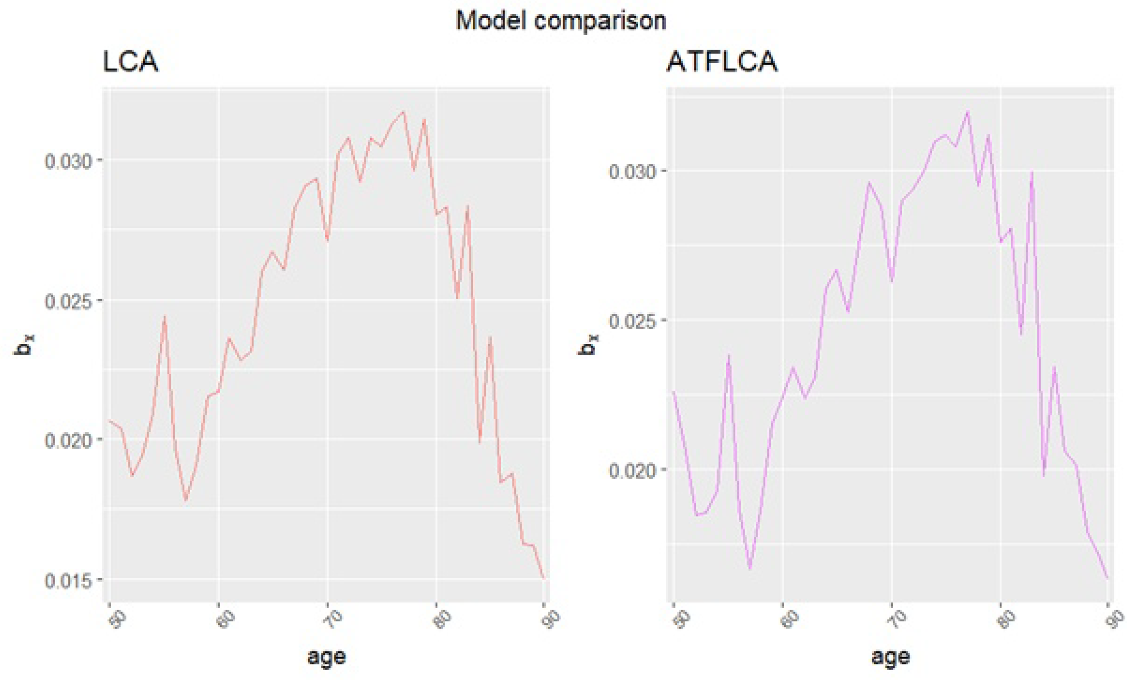
Following the Poisson log-bilinear Lee–Carter framework, both the LCA and ATFLCA models are estimated via maximum likelihood (MLE). Figure 1, Figure 2, Figure 3, Figure 4 and Figure 5 present the comparison of parameter estimates obtained for the LCA and ATFLCA models.

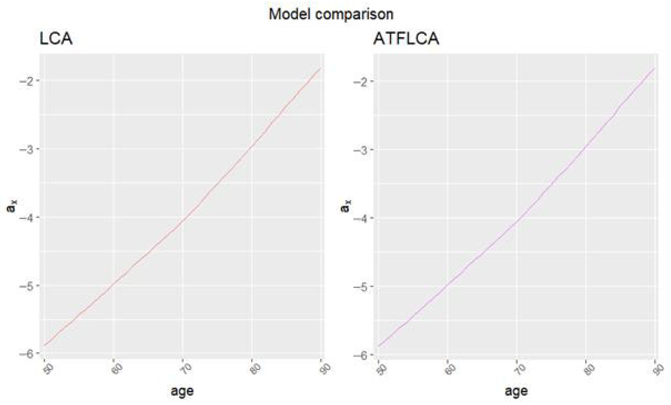
The parameter $a_x$ represents the average of log-specific mortality rates. Figure 1 shows that $a_x$ does not depend on frailty; therefore, its estimation is identical for both the LCA and ATFLCA models.

The parameter $b_x$ represents the mortality effect due to age. Figure 2 shows that this parameter is influenced by the frailty factor. In particular, both models exhibit a reversed U-shaped pattern with a peak in the mid-70s, but the ATFLCA model displays lower values at middle ages and higher values at very old ages compared to the LCA model. This indicates a stronger impact of ageing on the general mortality trend, measured by $k_t$. Consequently, the ATFLCA model yields more optimistic projections for mortality rates at older ages, corresponding to a (particular) negative $k_t$.

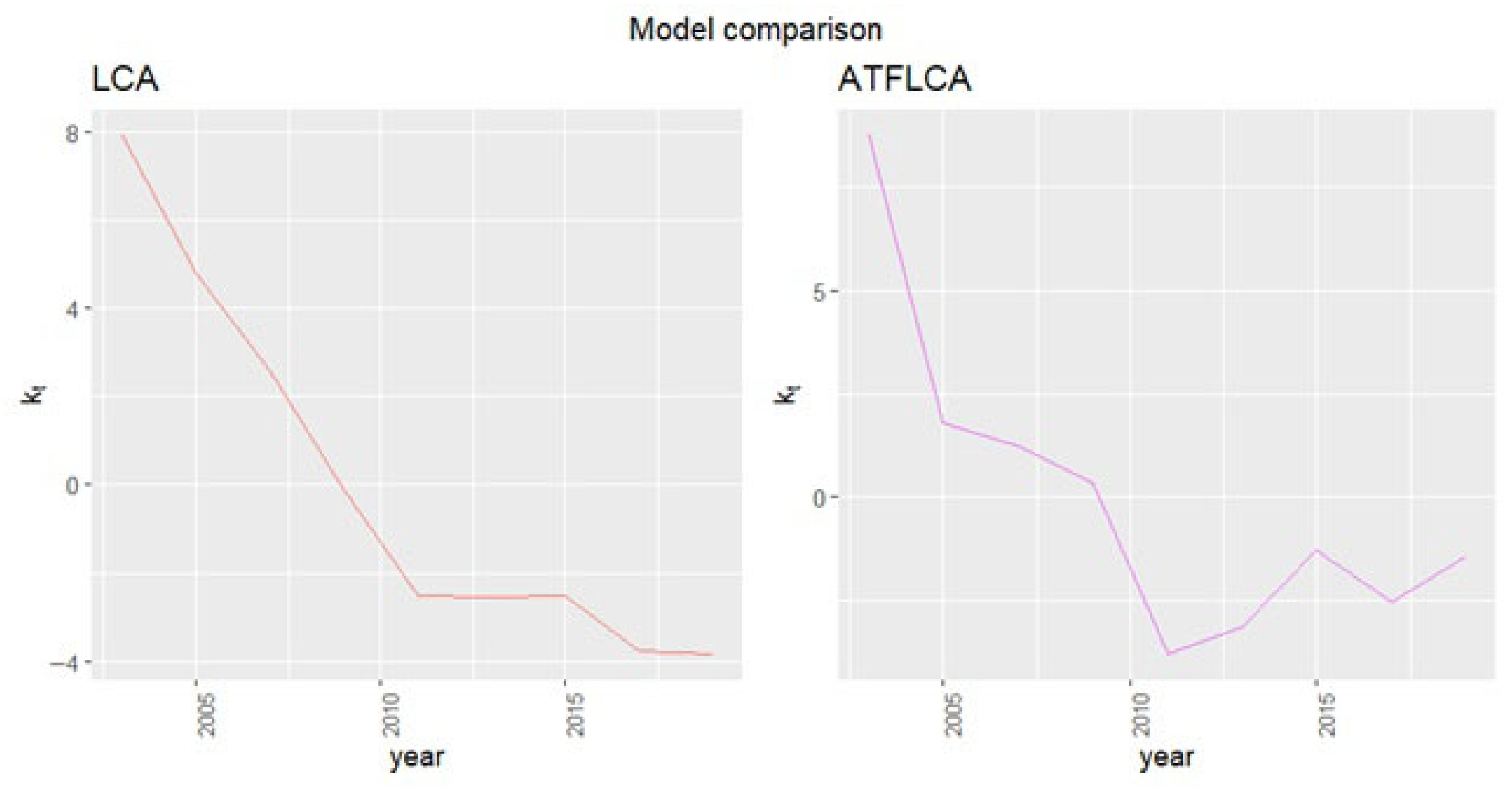
The parameter $k_t$ represents the general trend of mortality. Figure 3 shows a decreasing mortality trend for both models. However, a notable difference emerges in the period 2011–2014: while the LCA curve is flat, the ATFLCA curve increases, indicating a deterioration in longevity improvements. This result is particularly relevant, as it suggests a possible cause–effect relationship between co-morbidity and longevity that the standard LCA model is unable to capture.

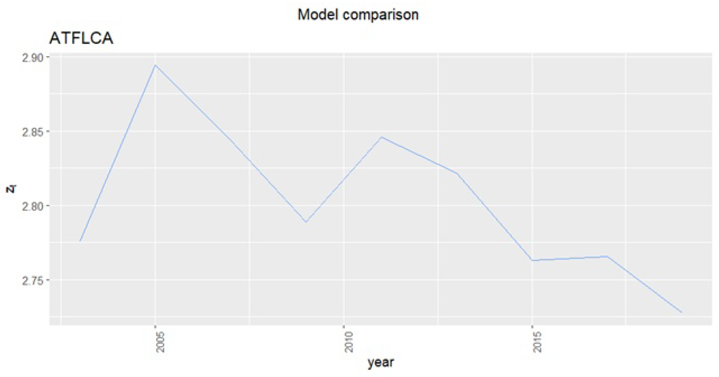
The parameter $z_t$ represents the average frailty score over time. Figure 4 shows a generally decreasing trend, with some upward peaks—most notably in 2005 and 2011—mirroring the behaviour observed in the $k_t$ parameter. This suggests that the evolution of $k_t$ is influenced by the dynamics of $z_t$. The differing behaviour of $k_t$ in the LCA and ATFLCA models can therefore be interpreted as a correction introduced by incorporating an exogenous factor affecting mortality, namely frailty.

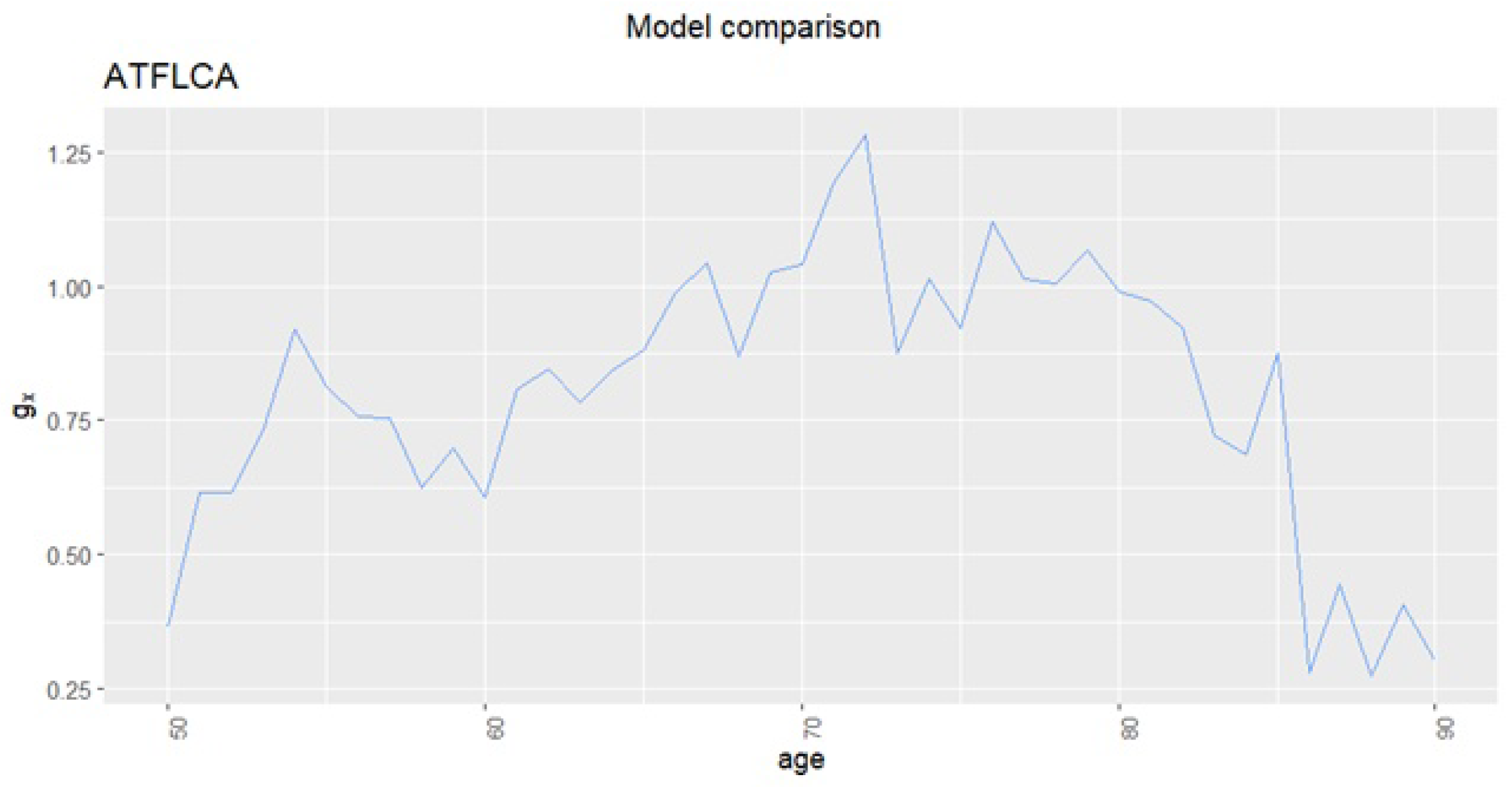
The parameter $g_x$ captures the age-specific frailty effect. As shown in Figure 5, $g_x$ exhibits a reversed U-shaped pattern, similar to the behaviour of $b_x$, with a peak in the mid-70s and very low values beyond the mid-80s. This result indicates that co-morbidity incidence increases through middle age, reaches its highest impact around age 70, and then decreases, becoming negligible at very advanced ages.

To assess the goodness of fit of the model,

Table 2. Model information criteria.

Model	Deviance	Test vs. LCA	p-Value	AIC	AICc	BIC
LCA	20.443	-	-	−241.447	−240.799	−236.307
ATFLCA	23.395	5.903	0.05227	−248.505	−246.791	−239.938

shows the deviance test of the ATFLCA vs. the LCA model and the information criteria based on deviance. We consider the Akaike Information Criterion (AIC), small-sample-corrected AIC (AICc) and Bayesian Information Criterion (BIC).

Table 2 shows that the ATFLCA model provides an overall improved fit according to all information criteria (AIC, AICc, and BIC), despite exhibiting a higher deviance compared to the baseline LCA specification. This reflects the standard trade-off between goodness of fit and model complexity, as the ATFLCA model introduces additional parameters to capture exogenous frailty effects. The likelihood ratio test is performed by considering the LCA model as the restricted model nested within the more general ATFLCA specification. The resulting p-value of 0.052 suggests that the inclusion of the exogenous frailty component provides a marginally significant improvement in explaining mortality dynamics. In a broader sense, the results suggest that augmenting the Lee–Carter framework with an exogenous covariate may enhance its ability to capture additional variation in mortality dynamics, improving the overall explanatory performance of the model.

To obtain mortality projections, we construct trajectories for $k_t$ to estimate the LCA projections, and for both $k_t$ and $z_t$ to estimate the ATFLCA projections. In both models, the trajectories of $k_t$ are generated using a random walk with drift. For $z_t$, the Box–Jenkins procedure indicates that the most appropriate specification for projection is also a random walk with drift. To ensure robustness, projections are based on 10,000 simulated paths for $k_t$ and $z_t$.

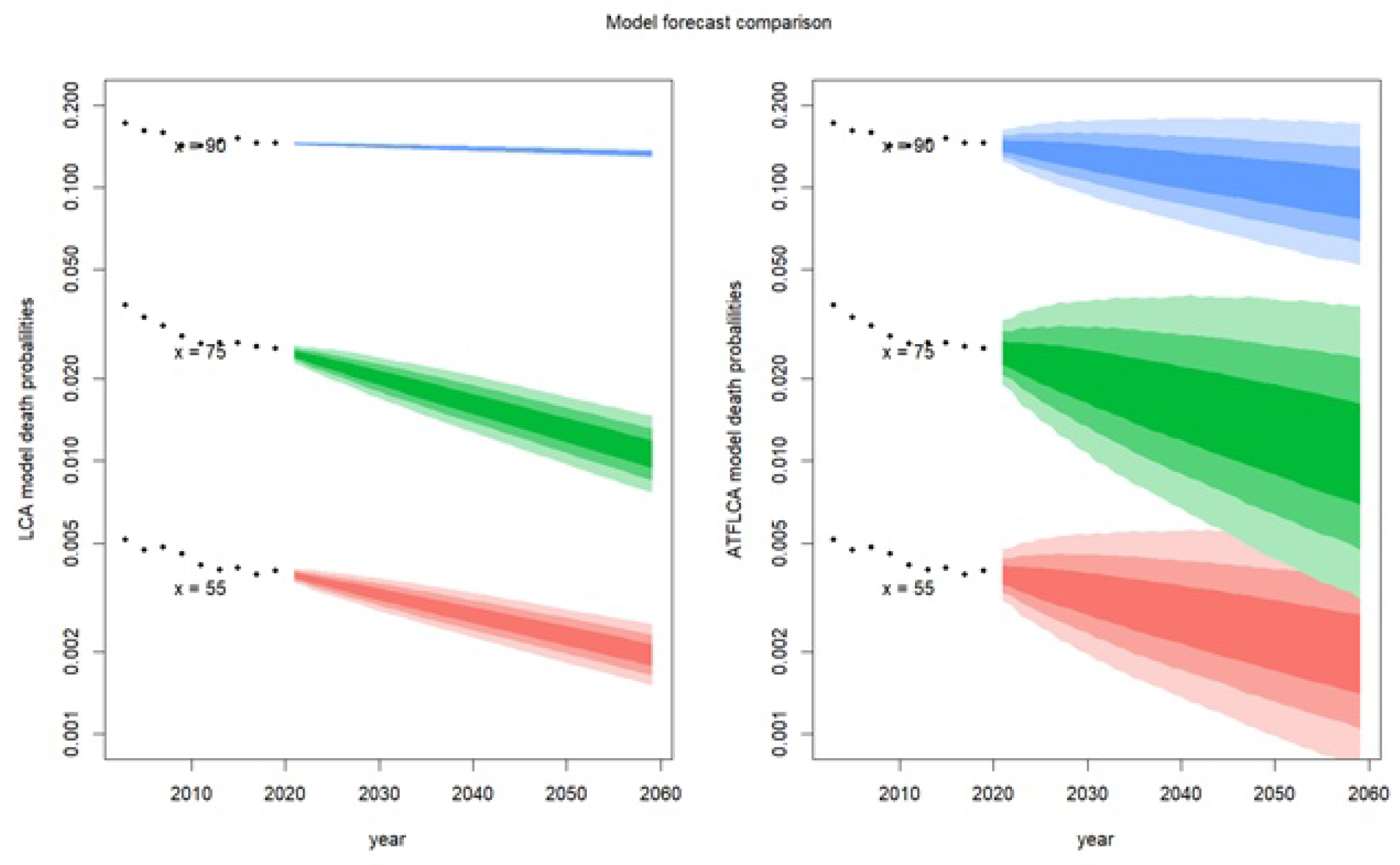
Figure 6 displays the projected log-death rates at ages 55, 75, and 90, with 50%, 80%, and 95% confidence intervals. The projections extend 40 years ahead, covering the period 2021–2061. Figure 6 shows that, although the projected mortality patterns are broadly similar across models, the ATFLCA model exhibits substantially higher volatility than the LCA one. This behaviour follows directly from the ATFLCA functional structure, which incorporates two stochastic temporal components: the general mortality trend $k_t$ and the average frailty trend $z_t$. The inclusion of frailty allows the model to capture heterogeneity in mortality dynamics, but it also introduces an additional source of uncertainty. As a result, the total volatility of the ATFLCA projections reflects the combined effect of the variances associated with both stochastic trends—the evolution of overall mortality and the evolution of population frailty.

Using the projected mortality paths obtained from the fitted models, we compute the annuity values and portfolio cash flows according to (7) and (8). The two hedging instruments are then evaluated through the payoff and cost structures introduced in Section 2.3 and Section 2.4.

3.3. De-Risking Strategies Under the LCA Scenario

Using a demographic technical basis derived from the LCA model, and assuming a flat rate of return on assets $j(t-1,t)=r=0.02$ for all t, the initial portfolio liabilities amount to

$$V_0=\mathrm{168,094},$$

while the total portfolio single premium is

$$P=\mathrm{170,326}.$$

We set the initial asset value $A_0$ equal to the total portfolio single premium.

Based on 10,000 simulations, we compute the evolution of unfunded liabilities without hedging ($U{L}_t$) and with hedging ($U{L}_t^j$) for both longevity options ($j=\mathrm{LO}$, with $h^{\mathrm{LO}}=1$) and longevity swaps ($j=\mathrm{LS}$, with $h^{\mathrm{LS}}=1$). The total unexpected losses ($TUL$, $TU{L}^{\mathrm{LO}}$, $TU{L}^{\mathrm{LS}}$) and the total portfolio costs ($TPC$, $TP{C}^{\mathrm{LO}}$, $TP{C}^{\mathrm{LS}}$) are computed according to Equations (30) and (10), respectively. The following assumptions are used in the evaluation:

• The default probability of the hedging provider is set to $0.1\%$ for both LO and LS: $p^{\mathrm{LO}}=p^{\mathrm{LS}}=0.001$.
• The default probability of the hedging buyer is set to $1\%$.
• The risk premium for the longevity option, ${\delta }^{\mathrm{LO}}$, is $2\%$.
• The longevity swap is assumed to be fully collateralised. We assume ${\delta }_s^{hb}$ constant and equal to the hedge buyer’s default intensity, while ${\delta }_s^{hs}={\delta }_s^{hb}+\Delta$, where $\Delta$ is the difference between hedge buyer and hedge provider default probabilities. Under these assumptions, the swap risk premium is $\pi =-0.0021$. This value is obtained by imposing $H{P}_0^{\mathrm{LS}}=0$ in (23) under the parametrisation described above and solving numerically for $\pi$. The negative sign is consistent with the results reported in (Biffis et al. 2016): under full bilateral collateralisation and asymmetric default risk, equilibrium swap rates may fall below best-estimate survival probabilities, reflecting the higher funding costs borne by the riskier counterparty and the interaction between collateral outflows and funding costs.
• The penalty factors in the $TPC$ equation are set to ${\psi }_1={\psi }_2=0.2$.

The results are reported in

Table 3. Portfolio results with and without de-risking strategies ($h^{\mathrm{LO}}=1$ or $h^{\mathrm{LS}}=1$). LCA scenario.

	No Hedging	$\mathit{j}=\mathbf{LO}$	$\mathit{j}=\mathbf{LS}$
$H{C}^j$	0.00	27.60	−357.81
$H{P}^j$	0.00	1407.59	0.00
${\mathbb{E}}^{\mathbb{P}}\left[TUL\right]$	−2232.27	−2204.67	−2642.93
${\mathrm{CVaR}}_{99.5\%}\left[TUL\right]$	7163.44	−616.22	−1060.58
${\mathbb{E}}^{\mathbb{P}}\left[TPC\right]$	−1481.08	−1210.40	−1939.38

.

Without hedging, ${\mathbb{E}}^{\mathbb{P}}\left[TUL\right]$ is negative, indicating an expected profit, but the portfolio is characterised by a positive ${\mathrm{CVaR}}_{99.5\%}\left[TUL\right]$ (with an average loss beyond the 99.5% VaR equal to $7163.44$, approximately $4.2\%$ of the reserve value at $t=0$). The penalty factors ${\psi }_1$ and ${\psi }_2$ reduce the profit, although ${\mathbb{E}}^{\mathbb{P}}\left[TPC\right]$ remains negative (even after penalisation, expected capital outflows exceed expected capital inflows).

When an LO hedging strategy is introduced, ${\mathbb{E}}^{\mathbb{P}}\left[TUL\right]$ increases (though it remains negative), whereas ${\mathrm{CVaR}}_{99.5\%}\left[TUL\right]$ is drastically reduced and becomes negative. The expected total cost, ${\mathbb{E}}^{\mathbb{P}}\left[TPC\right]$, also increases but stays negative.

When an LS hedging strategy is introduced, ${\mathbb{E}}^{\mathbb{P}}\left[TUL\right]$ decreases (due to the negative value of $\pi$), and ${\mathrm{CVaR}}_{99.5\%}\left[TUL\right]$ is reduced and becomes negative. The expected total cost ${\mathbb{E}}^{\mathbb{P}}\left[TPC\right]$ also decreases. We note that the swap hedging strategy has a negative hedging cost, $H{C}^{\mathrm{LS}}$.

We next determine the optimal hedge ratios by solving the optimisation problems in (29) and (31), using the cost and risk measures defined in Section 2.5. The following constraints for ${\mathbb{E}}^{\mathbb{P}}\left[TPC\right]$ and ${\mathrm{CVaR}}_{99.5\%}\left[TUL\right]$ are adopted:

• The maximum level c for the expected total cost of strategy j is set relative to its initial value (without hedging): $c=0.5·{\mathbb{E}}^{\mathbb{P}}\left[TPC\right].$
• The maximum level u for ${\mathrm{CVaR}}_{99.5\%}\left[TUL\right]$ is set relative to its initial value (without hedging): $u=0.5·{\mathrm{CVaR}}_{99.5\%}\left[TUL\right].$

The numerical results of the optimisation problems and the sensitivity analyses with respect to the relevant parameters (the proportional risk premium ${\delta }^{\mathrm{LO}}$, the swap risk premium $\pi$, the counterparty default probabilities $p^{\mathrm{LO}}$ and $p^{\mathrm{LS}}$, and the penalty factors ${\psi }_1$, ${\psi }_2$) are reported in the following tables.

From

Table 4. Option strategies obtained by minimising ${\mathbb{E}}^{\mathbb{P}}\left[TP{C}^{\mathrm{LO}}\right]$ subject to the CVaR constraint on total unfunded liabilities (Equation (29)), under different proportional risk premia (${\delta }^{\mathrm{LO}}$) and counter-party default probabilities ($p^{\mathrm{LO}}$). LCA scenario.

	${\mathit{\psi }}_1={\mathit{\psi }}_2=20\%$
${\delta }^{\mathrm{LO}}$	1%			2%			4%
$p^{\mathrm{LO}}$	0.00%	0.10%	0.50%	0.00%	0.10%	0.50%	0.00%	0.10%	0.50%
$h^{\mathrm{LO}}$	44.9%	45.9%	50.2%	45.0%	46.0%	50.3%	45.2%	46.2%	50.5%
$H{C}^{\mathrm{LO}}$	6.3	6.3	6.4	12.7	12.7	12.7	25.5	25.5	25.5
$H{P}^{\mathrm{LO}}$	640.2	640.4	641.2	647.7	647.9	648.7	662.8	663.0	663.8
${\mathbb{E}}^{\mathbb{P}}{\left[TUL\right]}^{\mathrm{LO}}$	−2225.9	−2225.9	−2225.9	−2219.6	−2219.6	−2219.6	−2206.8	−2206.8	−2206.7
${\mathrm{CVaR}}_{99.5\%}{\left[TUL\right]}^{\mathrm{LO}}$	3581.7	3581.7	3581.7	3581.7	3581.7	3581.7	3581.7	3581.7	3581.7
${\mathbb{E}}^{\mathbb{P}}{\left[TPC\right]}^{\mathrm{LO}}$	−1449.9	−1450.2	−1451.2	−1442.0	−1442.3	−1443.3	−1426.2	−1426.5	−1427.5

, we observe that the optimal strategy minimizing ${\mathbb{E}}^{\mathbb{P}}\left[TP{C}^{\mathrm{LO}}\right]$ is obtained with LO shares between $44\%$ and $50\%$. The results show that the cost minimisation strategy is affected by the acceptable CVaR target level: in all scenarios, the CVaR reaches the maximum admissible value, equal to one half of its initial level. It is also interesting to note that $h^{\mathrm{LO}}$ is influenced by the probability of failure of the hedge provider (a higher probability of failure reduces the effectiveness of the hedging strategy in lowering CVaR, thus requiring a higher $h^{\mathrm{LO}}$), while it is only marginally affected by the risk premium.

From

Table 5. Option strategies obtained by minimising ${\mathrm{CVaR}}_{99.5\%}\left[TU{L}^{\mathrm{LO}}\right]$ subject to the constraint on expected total portfolio cost (Equation (31)), under different proportional risk premia (${\delta }^{\mathrm{LO}}$) and counter-party default probabilities ($p^{\mathrm{LO}}$). LCA scenario.

	${\mathit{\psi }}_1={\mathit{\psi }}_2=20\%$
${\delta }^{\mathrm{LO}}$	1%			2%			4%
$p^{\mathrm{LO}}$	0.00%	0.10%	0.50%	0.00%	0.10%	0.50%	0.00%	0.10%	0.50%
$h^{\mathrm{LO}}$	100.0%	100.0%	100.0%	100.0%	100.0%	100.0%	100.0%	100.0%	100.0%
$H{C}^{\mathrm{LO}}$	14.1	13.8	12.6	28.2	27.6	25.3	56.4	55.2	50.5
$H{P}^{\mathrm{LO}}$	1424.9	1393.8	1276.3	1439.0	1407.6	1289.0	1467.3	1435.2	1314.2
${\mathbb{E}}^{\mathbb{P}}{\left[TUL\right]}^{\mathrm{LO}}$	−2218.2	−2218.5	−2219.6	−2204.1	−2204.7	−2207.0	−2175.8	−2177.1	−2181.7
${\mathrm{CVaR}}_{99.5\%}{\left[TUL\right]}^{\mathrm{LO}}$	−807.3	−630.0	38.8	−793.2	−616.2	51.4	−765.0	−588.6	76.7
${\mathbb{E}}^{\mathbb{P}}{\left[TPC\right]}^{\mathrm{LO}}$	−1215.4	−1227.0	−1269.9	−1198.5	−1210.4	−1254.7	−1164.6	−1177.3	−1224.4

, we observe that the optimal strategy minimizing ${\mathrm{CVaR}}_{99.5\%}\left[TU{L}^{\mathrm{LO}}\right]$ is obtained with an LO share equal to $100\%$, meaning a complete transfer of longevity risk. As the probability of failure of the hedge provider increases, the de-risking strategy becomes less effective, leading to higher CVaR values, while the results are only marginally affected by the level of the risk premium.

From

Table 6. Swap strategies obtained by minimising ${\mathbb{E}}^{\mathbb{P}}\left[TP{C}^{\mathrm{LS}}\right]$ subject to the CVaR constraint on total unfunded liabilities (Equation (29)), under different hedge provider default probabilities ($p^{\mathrm{LS}}$) and proportional risk premia (${\pi }^{\mathrm{LS}}$). LCA scenario.

	${\mathit{\psi }}_1={\mathit{\psi }}_2=20\%$
$p^{\mathrm{LS}}$	0.00%	0.10%	0.50%
${\pi }^{\mathrm{LS}}$	−0.24%	−0.22%	−0.12%
$h^{\mathrm{LS}}$	100.0%	100.0%	100.0%
$H{C}^{\mathrm{LS}}$	−404.87	−357.81	−184.96
${\mathbb{E}}^{\mathbb{P}}{\left[TUL\right]}^{\mathrm{LS}}$	−2730.06	−2689.07	−2523.17
${\mathrm{CVaR}}_{99.5\%}{\left[TUL\right]}^{\mathrm{LS}}$	−1561.73	−1264.69	−460.14
${\mathbb{E}}^{\mathbb{P}}{\left[TPC\right]}^{\mathrm{LS}}$	−2012.80	−1983.37	−1860.75

we observe that the optimal strategy minimizing ${\mathbb{E}}^{\mathbb{P}}\left[TP{C}^{\mathrm{LS}}\right]$ is consistently achieved through a full risk transfer, with $h^{\mathrm{LS}}=100\%$. However, its effectiveness is affected by the probability of failure of the hedge provider: a higher failure probability leads to larger values of both $\mathrm{CVaR}$ and ${\mathbb{E}}^{\mathbb{P}}\left[TP{C}^{\mathrm{LS}}\right]$. The results also show that, in this case, the cost minimisation strategy is not constrained by the CVaR requirement.

The results in

Table 7. Swap strategies obtained by minimising ${\mathrm{CVaR}}_{99.5\%}\left[TU{L}^{\mathrm{LS}}\right]$ subject to the constraint on expected total portfolio cost (Equation (31)), under different hedge provider default probabilities ($p^{\mathrm{LS}}$) and proportional risk premia (${\pi }^{\mathrm{LS}}$). LCA scenario.

	${\mathit{\psi }}_1={\mathit{\psi }}_2=20\%$
$p^{\mathrm{LS}}$	0.00%	0.10%	0.50%
${\pi }^{\mathrm{LS}}$	−0.24%	−0.22%	−0.12%
$h^{\mathrm{LS}}$	89.7%	87.2%	87.4%
$H{C}^{\mathrm{LS}}$	−363.06	−312.13	−161.73
${\mathbb{E}}^{\mathbb{P}}{\left[TUL\right]}^{\mathrm{LS}}$	−2678.66	−2630.75	−2486.64
${\mathrm{CVaR}}_{99.5\%}{\left[TUL\right]}^{\mathrm{LS}}$	−2511.27	−1914.04	−1297.03
${\mathbb{E}}^{\mathbb{P}}{\left[TPC\right]}^{\mathrm{LS}}$	−1997.35	−1966.39	−1856.12

show that the optimal strategy minimizing ${\mathrm{CVaR}}_{99.5\%}\left[TU{L}^{\mathrm{LS}}\right]$ is achieved with an LS share close to, but not exactly, $100\%$. As in the previous analyses, a higher probability of failure of the hedge provider reduces the effectiveness of the de-risking strategy, leading to higher CVaR values.

Table 8. Option strategies obtained by minimising ${\mathbb{E}}^{\mathbb{P}}\left[TP{C}^{\mathrm{LO}}\right]$ subject to the CVaR constraint on total unfunded liabilities (Equation (29)), under different penalty factors (${\psi }_1,{\psi }_2$). LCA scenario.

	${\mathit{\delta }}^{\mathbf{LO}}=2\%$
	${\mathit{p}}^{\mathbf{LO}}\mathbf{=}\mathbf{0.10}\mathbf{\%}$
${\psi }_1$	10%			20%			30%
${\psi }_2$	10%	20%	30%	10%	20%	30%	10%	20%	30%
$h^{\mathrm{LO}}$	46.0%	46.0%	46.0%	46.0%	46.0%	46.0%	46.0%	46.0%	46.0%
$H{C}^{\mathrm{LO}}$	12.7	12.7	12.7	12.7	12.7	12.7	12.7	12.7	12.7
$H{P}^{\mathrm{LO}}$	647.9	647.9	647.9	647.9	647.9	647.9	647.9	647.9	647.9
${\mathbb{E}}^{\mathbb{P}}{\left[TUL\right]}^{\mathrm{LO}}$	−2219.6	−2219.6	−2219.6	−2219.6	−2219.6	−2219.6	−2219.6	−2219.6	−2219.6
${\mathrm{CVaR}}_{99.5\%}{\left[TUL\right]}^{\mathrm{LO}}$	3581.7	3581.7	3581.7	3581.7	3581.7	3581.7	3581.7	3581.7	3581.7
${\mathbb{E}}^{\mathbb{P}}{\left[TPC\right]}^{\mathrm{LO}}$	−1830.9	−1525.6	−1220.3	−1747.6	−1442.3	−1137.0	−1664.3	−1359.0	−1053.6

reports the values of $h^{\mathrm{LO}}$ that minimise ${\mathbb{E}}^{\mathbb{P}}\left[TP{C}^{\mathrm{LO}}\right]$ under different assumptions for the penalty factors $({\psi }_1,{\psi }_2)$. The results show that the optimal $h^{\mathrm{LO}}$ remains unchanged across all scenarios, even though ${\mathbb{E}}^{\mathbb{P}}\left[TP{C}^{\mathrm{LO}}\right]$ varies with the penalty levels. This invariance arises because the cost minimisation strategy is constrained by the acceptable CVaR target level, equal to $3581.72$.

In

Table 9. Option strategies obtained by minimising ${\mathrm{CVaR}}_{99.5\%}\left[TU{L}^{\mathrm{LO}}\right]$ subject to the constraint on expected total portfolio cost (Equation (31)), under different penalty factors (${\psi }_1,{\psi }_2$). LCA scenario.

	${\mathit{\delta }}^{\mathbf{LO}}=2\%$
	${\mathit{p}}^{\mathbf{LO}}\mathbf{=}\mathbf{0.10}\mathbf{\%}$
${\psi }_1$	10%			20%			30%
${\psi }_2$	10%	20%	30%	10%	20%	30%	10%	20%	30%
$h^{\mathrm{LO}}$	100.0%	100.0%	100.0%	100.0%	100.0%	100.0%	100.0%	100.0%	100.0%
$H{C}^{\mathrm{LO}}$	27.6	27.6	27.6	27.6	27.6	27.6	27.6	27.6	27.6
$H{P}^{\mathrm{LO}}$	1407.6	1407.6	1407.6	1407.6	1407.6	1407.6	1407.6	1407.6	1407.6
${\mathbb{E}}^{\mathbb{P}}{\left[TUL\right]}^{\mathrm{LO}}$	−2204.7	−2204.7	−2204.7	−2204.7	−2204.7	−2204.7	−2204.7	−2204.7	−2204.7
${\mathrm{CVaR}}_{99.5\%}{\left[TUL\right]}^{\mathrm{LO}}$	−616.2	−616.2	−616.2	−616.2	−616.2	−616.2	−616.2	−616.2	−616.2
${\mathbb{E}}^{\mathbb{P}}{\left[TPC\right]}^{\mathrm{LO}}$	−1707.6	−1348.7	−989.9	−1569.2	−1210.4	−851.6	−1430.9	−1072.1	−713.3

, the CVaR minimisation criterion always leads to a full longevity option hedge, with $h^{\mathrm{LO}}=100\%$, for all combinations of the penalty factors ${\psi }_1$ and ${\psi }_2$. This confirms the finding already observed in Table 5 and indicates that, in the LCA scenario considered here, the full hedge is the strategy that minimises tail risk, with the cost constraint never binding in the cases reported. Since the penalty factors enter the total portfolio cost but do not affect the distribution of total unfunded liabilities, both ${\mathbb{E}}^{\mathbb{P}}{\left[TUL\right]}^{\mathrm{LO}}$ and ${\mathrm{CVaR}}_{99.5\%}{\left[TUL\right]}^{\mathrm{LO}}$ remain unchanged across the table, whereas only ${\mathbb{E}}^{\mathbb{P}}{\left[TPC\right]}^{\mathrm{LO}}$ varies.

The results in

Table 10. Swap strategies obtained by minimising ${\mathbb{E}}^{\mathbb{P}}\left[TP{C}^{\mathrm{LS}}\right]$ subject to the CVaR constraint on total unfunded liabilities (Equation (29)), under different penalty factors (${\psi }_1,{\psi }_2$). LCA scenario.

	${\mathit{\pi }}^{\mathbf{LS}}=-0.22\%$
	${\mathit{p}}^{\mathbf{LS}}\mathbf{=}\mathbf{0.10}\mathbf{\%}$
${\psi }_1$	10%			20%			30%
${\psi }_2$	10%	20%	30%	10%	20%	30%	10%	20%	30%
$h^{\mathrm{LS}}$	100.0%	100.0%	100.0%	100.0%	100.0%	98.4%	100.0%	100.0%	89.7%
$H{C}^{\mathrm{LS}}$	−357.8	−357.8	−357.8	−357.8	−357.8	−352.1	−357.8	−357.8	−321.1
${\mathbb{E}}^{\mathbb{P}}{\left[TUL\right]}^{\mathrm{LS}}$	−2689.1	−2689.1	−2689.1	−2689.1	−2689.1	−2681.8	−2689.1	−2689.1	−2642.2
${\mathrm{CVaR}}_{99.5\%}{\left[TUL\right]}^{\mathrm{LS}}$	−1264.7	−1264.7	−1264.7	−1264.7	−1264.7	−1377.6	−1264.7	−1264.7	−1837.1
${\mathbb{E}}^{\mathbb{P}}{\left[TPC\right]}^{\mathrm{LS}}$	−2336.2	−2025.4	−1714.5	−2294.3	−1983.4	−1672.6	−2252.3	−1941.4	−1634.5

show that the optimal longevity swap strategy for minimizing ${\mathbb{E}}^{\mathbb{P}}\left[TP{C}^{\mathrm{LS}}\right]$ corresponds to a full risk transfer, with $h^{\mathrm{LS}}=100\%$, whenever both penalty factors are equal to or below $20\%$. When both penalty factors reach $30\%$, the optimal share decreases to $89.7\%$. Moreover, the results indicate that ${\psi }_2$ exerts a slightly stronger influence on the strategy than ${\psi }_1$.

In the case of CVaR minimisation (

Table 11. Swap strategies obtained by minimising ${\mathrm{CVaR}}_{99.5\%}\left[TU{L}^{\mathrm{LS}}\right]$ subject to the constraint on expected total portfolio cost (Equation (31)), under different penalty factors (${\psi }_1,{\psi }_2$). LCA scenario.

	${\mathit{\pi }}^{\mathbf{LS}}=-0.22\%$
	${\mathit{p}}^{\mathbf{LS}}\mathbf{=}\mathbf{0.10}\mathbf{\%}$
${\psi }_1$	10%			20%			30%
${\psi }_2$	10%	20%	30%	10%	20%	30%	10%	20%	30%
$h^{\mathrm{LS}}$	87.2%	87.2%	87.2%	87.2%	87.2%	87.2%	87.2%	87.2%	87.2%
$H{C}^{\mathrm{LS}}$	−312.1	−312.1	−312.1	−312.1	−312.1	−312.1	−312.1	−312.1	−312.1
${\mathbb{E}}^{\mathbb{P}}{\left[TUL\right]}^{\mathrm{LS}}$	−2630.8	−2630.8	−2630.8	−2630.8	−2630.8	−2630.8	−2630.8	−2630.8	−2630.8
${\mathrm{CVaR}}_{99.5\%}{\left[TUL\right]}^{\mathrm{LS}}$	−1914.0	−1914.0	−1914.0	−1914.0	−1914.0	−1914.0	−1914.0	−1914.0	−1914.0
${\mathbb{E}}^{\mathbb{P}}{\left[TPC\right]}^{\mathrm{LS}}$	−2298.6	−2001.0	−1703.3	−2264.0	−1966.4	−1668.8	−2229.5	−1931.8	−1634.2

), the optimal strategy consistently corresponds to an LS share of $h^{\mathrm{LS}}=87.2\%$. This occurs because such a hedging level minimises the $\mathrm{CVaR}$, while the constraint on ${\mathbb{E}}^{\mathbb{P}}\left[TP{C}^{\mathrm{LS}}\right]$ does not restrict the strategy for any of the penalty factor combinations considered.

When considering both risk transfer instruments simultaneously, the results indicate distinct optimal behaviours depending on the chosen objective. When the objective is to minimise ${\mathbb{E}}^{\mathbb{P}}\left[TPC\right]$ (

Table 12. Mixed option and swap strategies obtained by minimising ${\mathbb{E}}^{\mathbb{P}}\left[TP{C}^{(\mathrm{LO},\mathrm{LS})}\right]$ subject to the CVaR constraint on total unfunded liabilities (Equation (29)), under different counter-party default probabilities ($p^{\mathrm{LO}}$ and $p^{\mathrm{LS}}$) and proportional risk premia (${\delta }^{\mathrm{LO}}$ and ${\pi }^{\mathrm{LS}}$). LCA scenario.

	${\mathit{\psi }}_1={\mathit{\psi }}_2=20\%$
$p^{\mathrm{LO}}=p^{\mathrm{LS}}$	0%			0.1%			0.5%
${\pi }^{\mathrm{LS}}$	−0.24%			−0.22%			−0.12%
${\delta }^{\mathrm{LO}}$	0%	2%	4%	0%	2%	4%	0%	2%	4%
$h^{\mathrm{LO}}$	0.0%	0.0%	0.0%	0.0%	0.0%	0.0%	4.7%	4.0%	0.9%
$h^{\mathrm{LS}}$	100.0%	100.0%	100.0%	100.0%	100.0%	100.0%	95.3%	96.0%	99.1%
$H{C}^{(\mathrm{LO},\mathrm{LS})}$	−404.9	−404.9	−404.9	−357.8	−357.8	−357.8	−175.6	−176.6	−182.8
$H{P}^{\mathrm{LO}}$	0.0	0.0	0.0	0.0	0.0	0.0	60.6	51.2	12.0
${\mathbb{E}}^{\mathbb{P}}{\left[TUL\right]}^{(\mathrm{LO},\mathrm{LS})}$	−2730.1	−2730.1	−2730.1	−2689.1	−2689.1	−2689.1	−2508.8	−2510.6	−2520.1
${\mathrm{CVaR}}_{99.5\%}{\left[TUL\right]}^{(\mathrm{LO},\mathrm{LS})}$	−1561.7	−1561.7	−1561.7	−1264.7	−1264.7	−1264.7	−754.5	−705.9	−516.6
${\mathbb{E}}^{\mathbb{P}}{\left[TPC\right]}^{(\mathrm{LO},\mathrm{LS})}$	−2012.8	−2012.8	−2012.8	−1983.4	−1983.4	−1983.4	−1861.8	−1861.3	−1860.8

), the optimal strategy is to rely exclusively on the longevity swap (LS) as long as the failure probability of the hedge provider is zero or negligible. A partial use of the longevity option (LO) appears only when both $p^{\mathrm{LO}}$ and $p^{\mathrm{LS}}$ are equal to $0.5\%$. Even in this case, however, the optimal LO shares remain very small and decrease as ${\delta }^{\mathrm{LO}}$ increases.

When the objective is to minimise $\mathrm{CVaR}$ (

Table 13. Mixed option and swap strategies obtained by minimising ${\mathrm{CVaR}}_{99.5\%}\left[TU{L}^{(\mathrm{LO},\mathrm{LS})}\right]$ subject to the constraint on expected total portfolio cost (Equation (31)), under different counter-party default probabilities ($p^{\mathrm{LO}}$ and $p^{\mathrm{LS}}$) and proportional risk premia (${\delta }^{\mathrm{LO}}$ and ${\pi }^{\mathrm{LS}}$). LCA scenario.

	${\mathit{\psi }}_1={\mathit{\psi }}_2=20\%$
$p^{\mathrm{LO}}=p^{\mathrm{LS}}$	0%			0.1%			0.5%
${\pi }^{\mathrm{LS}}$	−0.24%			−0.22%			−0.12%
${\delta }^{\mathrm{LO}}$	0%	2%	4%	0%	2%	4%	0%	2%	4%
$h^{\mathrm{LO}}$	1.6%	1.1%	0.7%	22.6%	22.3%	22.5%	27.6%	27.6%	27.5%
$h^{\mathrm{LS}}$	89.1%	89.2%	89.4%	73.2%	73.3%	73.2%	72.4%	72.4%	72.5%
$H{C}^{(\mathrm{LO},\mathrm{LS})}$	−360.5	−360.9	−361.3	−258.7	−256.0	−249.5	−130.4	−126.9	−120.2
$H{P}^{\mathrm{LO}}$	22.52	15.79	9.68	314.81	313.77	322.79	352.08	355.36	361.20
${\mathbb{E}}^{\mathbb{P}}{\left[TUL\right]}^{(\mathrm{LO},\mathrm{LS})}$	−2675.60	−2676.08	−2676.68	−2563.45	−2560.79	−2554.25	−2439.44	−2435.95	−2429.32
${\mathrm{CVaR}}_{99.5\%}{\left[TUL\right]}^{(\mathrm{LO},\mathrm{LS})}$	−2511.28	−2511.30	−2511.26	−2190.92	−2117.90	−2111.63	−1763.01	−1759.52	−1752.37
${\mathbb{E}}^{\mathbb{P}}{\left[TPC\right]}^{(\mathrm{LO},\mathrm{LS})}$	−1997.06	−1996.92	−1996.86	−1986.01	−1884.00	−1875.37	−1774.69	−1770.51	−1762.77

), the optimal strategy becomes a combination of both hedging instruments. The LS component is always dominant, but its optimal share decreases as $p^{\mathrm{LO}}$ and $p^{\mathrm{LS}}$ increase (and, consequently, as ${\pi }^{\mathrm{LS}}$ becomes less negative).

A notable feature of the results is the difference in total risk transfer between the two optimisation objectives. When minimizing ${\mathbb{E}}^{\mathbb{P}}\left[TPC\right]$, the optimal strategy always corresponds to full risk transfer, i.e., $h^{\mathrm{LO}}+h^{\mathrm{LS}}=100\%$. In contrast, when minimizing $\mathrm{CVaR}$, full risk transfer is optimal only when $p^{\mathrm{LO}}$ and $p^{\mathrm{LS}}$ are both equal to $0.5\%$. In all other scenarios, the optimal risk transfer is below $100\%$, though it always exceeds $90\%$.

3.4. De-Risking Strategies Under the ATFLCA Scenario

In the second part of this numerical application, the demographic technical bases are derived using the ATFLCA model (ATFLCA scenario). The parameters of the risk transfer instruments are kept equal to those adopted in the LCA scenario, namely:

$$p^{\mathrm{LO}}=p^{\mathrm{LS}}=0.1\%,{\delta }^{\mathrm{LO}}=2\%,{\psi }_1={\psi }_2=0.2.$$

Assuming full collateralisation of the longevity swap, the corresponding risk premium is $\pi =-0.0080$.

Under these assumptions, the results obtained are summarised in

Table 14. Portfolio results with and without de-risking strategies ($h^{\mathrm{LO}}=1$ or $h^{\mathrm{LS}}=1$). ATFLCA scenario.

	No Hedging	$\mathit{j}=\mathbf{LO}$	$\mathit{j}=\mathbf{LS}$
$H{C}^j$	0.00	102.82	−1328.20
$H{P}^j$	0.00	5,243.84	0.00
${\mathbb{E}}^{\mathbb{P}}\left[TUL\right]$	−2720.26	−2617.44	−4236.14
${\mathrm{CVaR}}_{99.5\%}\left[TUL\right]$	29,603.60	3283.01	2349.12
${\mathbb{E}}^{\mathbb{P}}\left[TPC\right]$	−299.17	261.40	−2265.73

.

Also in the ATFLCA scenario, without hedging the value of ${\mathbb{E}}^{\mathbb{P}}\left[TUL\right]$ is negative, indicating an expected profit. The quantity ${\mathbb{E}}^{\mathbb{P}}\left[TPC\right]$ is also negative. However, the portfolio exhibits a positive ${\mathrm{CVaR}}_{99.5\%}\left[TUL\right]$, with an average loss beyond the $99.5\%$ VaR equal to $\mathrm{29,603.60}$, i.e., more than $17\%$ of the reserve at $t=0$. The substantially greater variability in the simulated death probabilities produced by the ATFLCA model leads to a $\mathrm{CVaR}$ more than four times larger than that obtained under the LCA model, despite the reserves being very similar. It is therefore evident that, in this case, the introduction of de-risking strategies is essential.

When an LO hedging strategy is adopted, ${\mathbb{E}}^{\mathbb{P}}\left[TUL\right]$ increases (while remaining negative), and ${\mathrm{CVaR}}_{99.5\%}\left[TUL\right]$ is sharply reduced. The expected total cost ${\mathbb{E}}^{\mathbb{P}}\left[TPC\right]$ also increases and becomes positive. The LS hedging strategy, on the other hand, displays a negative hedging cost $H{C}^{\mathrm{LS}}$. Under the LS strategy, ${\mathbb{E}}^{\mathbb{P}}\left[TUL\right]$ decreases (due to the negative value of $\pi$), and ${\mathrm{CVaR}}_{99.5\%}\left[TUL\right]$ decreases even more than under the LO strategy. The expected total cost ${\mathbb{E}}^{\mathbb{P}}\left[TPC\right]$ also improves (i.e., decreases).

The optimisation problems defined in Equations (29) and (31) are then applied. The same constraints used in the LCA scenario are adopted:

• The maximum acceptable expected total cost for strategy j is set to $c=0.5·{\mathbb{E}}^{\mathbb{P}}\left[TPC\right]$.
• The maximum acceptable level of ${\mathrm{CVaR}}_{99.5\%}\left[TUL\right]$ is set to $u=0.5·{\mathrm{CVaR}}_{99.5\%}\left[TUL\right]$.

The numerical results of the optimisation problems, together with sensitivity analyses on the relevant parameters (proportional risk premium ${\delta }^{\mathrm{LO}}$, longevity swap risk premium $\pi$, counterparty default probabilities $p^{\mathrm{LO}}$ and $p^{\mathrm{LS}}$, and penalty factors ${\psi }_1,{\psi }_2$), are presented in the following tables.

From

Table 15. Option strategies obtained by minimising ${\mathbb{E}}^{\mathbb{P}}\left[TP{C}^{\mathrm{LO}}\right]$ subject to the CVaR constraint on total unfunded liabilities (Equation (29)), under different proportional risk premia (${\delta }^{\mathrm{LO}}$) and counter-party default probabilities ($p^{\mathrm{LO}}$). ATFLCA scenario.

	${\mathit{\psi }}_1={\mathit{\psi }}_2=20\%$
${\delta }^{\mathrm{LO}}$	1%			2%			4%
$p^{\mathrm{LO}}$	0.00%	0.10%	0.50%	0.00%	0.10%	0.50%	0.00%	0.10%	0.50%
$h^{\mathrm{LO}}$	54.8%	56.1%	61.8%	54.9%	56.2%	61.9%	55.1%	56.4%	62.1%
$H{C}^{\mathrm{LO}}$	28.79	28.85	29.07	57.69	57.81	58.26	115.84	116.06	116.97
$H{P}^{\mathrm{LO}}$	2907.86	2913.48	2936.13	2942.38	2948.07	2971.04	3011.81	3017.66	3041.27
${\mathbb{E}}^{\mathbb{P}}{\left[TUL\right]}^{\mathrm{LO}}$	−2691.47	−2691.41	−2691.19	−2662.57	−2662.46	−2662.01	−2604.42	−2604.20	−2603.29
${\mathrm{CVaR}}_{99.5\%}{\left[TUL\right]}^{\mathrm{LO}}$	14,801.80	14,801.80	14,801.80	14,801.80	14,801.80	14,801.80	14,801.80	14,801.80	14,801.80
${\mathbb{E}}^{\mathbb{P}}{\left[TPC\right]}^{\mathrm{LO}}$	−327.75	−328.66	−332.07	−292.27	−293.11	−296.27	−220.88	−221.60	−224.24

, we observe that the optimal strategy minimizing ${\mathbb{E}}^{\mathbb{P}}\left[TP{C}^{\mathrm{LO}}\right]$ is obtained with LO shares between 54% and 62%, noticeably higher than in the LCA scenario. As in the LCA case, the cost minimisation strategy is constrained by the acceptable CVaR level: in every scenario, the resulting ${\mathrm{CVaR}}_{99.5\%}\left[TUL\right]$ is exactly equal to 50% of its initial value. The results confirm that $h^{\mathrm{LO}}$ is strongly influenced by the probability of failure of the hedge provider: a higher default probability reduces the effectiveness of the hedging strategy in lowering the CVaR, therefore requiring a higher value of $h^{\mathrm{LO}}$. Conversely, the optimal LO share appears only marginally affected by the proportional risk premium.

From

Table 16. Option strategies obtained by minimising ${\mathrm{CVaR}}_{99.5\%}\left[TU{L}^{\mathrm{LO}}\right]$ subject to the constraint on expected total portfolio cost (Equation (31)), under different proportional risk premia (${\delta }^{\mathrm{LO}}$) and counter-party default probabilities ($p^{\mathrm{LO}}$). ATFLCA scenario.

	${\mathit{\psi }}_1={\mathit{\psi }}_2=20\%$
${\delta }^{\mathrm{LO}}$	1%			2%			4%
$p^{\mathrm{LO}}$	0.00%	0.10%	0.50%	0.00%	0.10%	0.50%	0.00%	0.10%	0.50%
$h^{\mathrm{LO}}$	72.4%	74.3%	82.4%	68.7%	70.5%	78.2%	61.7%	63.3%	70.1%
$H{C}^{\mathrm{LO}}$	38.06	38.21	38.80	72.21	72.48	73.57	129.69	130.13	131.89
$H{P}^{\mathrm{LO}}$	3844.51	3859.38	3918.90	3682.68	3696.53	3751.99	3711.87	3823.42	4329.17
${\mathbb{E}}^{\mathbb{P}}{\left[TUL\right]}^{\mathrm{LO}}$	−2682.20	−2682.05	−2681.46	−2648.05	−2647.78	−2646.69	−2590.57	−2590.13	−2583.87
${\mathrm{CVaR}}_{99.5\%}{\left[TUL\right]}^{\mathrm{LO}}$	10,034.01	9996.22	9851.09	11,077.66	11,043.92	10,913.58	13,032.42	13,007.74	12,914.70
${\mathbb{E}}^{\mathbb{P}}{\left[TPC\right]}^{\mathrm{LO}}$	−149.59	−149.58	−149.56	−149.59	−149.59	−149.56	−149.59	−149.58	−149.56

, we observe that the optimal strategy minimizing ${\mathrm{CVaR}}_{99.5\%}\left[TU{L}^{\mathrm{LO}}\right]$ is influenced by both the proportional risk premium and the probability of failure of the hedge provider. Specifically, the optimal LO share $h^{\mathrm{LO}}$ increases as ${\delta }^{\mathrm{LO}}$ increases, and it also increases as $p^{\mathrm{LO}}$ rises, reflecting the reduced effectiveness of the hedge in controlling downside risk when default risk is higher. The optimisation is always constrained by the requirement on ${\mathbb{E}}^{\mathbb{P}}\left[TPC\right]$. In all scenarios, ${\mathbb{E}}^{\mathbb{P}}\left[TPC\right]$ reaches exactly half of its initial value, indicating that the LO strategy is capped to prevent excessive increases in total expected costs. In other words, cost considerations bind the solution, limiting the extent of risk transfer even when a higher $h^{\mathrm{LO}}$ would further reduce the CVaR.

The results in

Table 17. Swap strategies obtained by minimising ${\mathbb{E}}^{\mathbb{P}}\left[TP{C}^{\mathrm{LS}}\right]$ subject to the CVaR constraint on total unfunded liabilities (Equation (29)), under different hedge provider default probabilities ($p^{\mathrm{LS}}$) and proportional risk premia (${\pi }^{\mathrm{LS}}$). ATFLCA scenario.

	${\mathit{\psi }}_1={\mathit{\psi }}_2=20\%$
$p^{\mathrm{LS}}$	0.00%	0.10%	0.50%
${\pi }^{\mathrm{LS}}$	−0.90%	−0.80%	−0.43%
$h^{\mathrm{LS}}$	100.0%	100.0%	100.0%
$H{C}^{\mathrm{LS}}$	−1502.74	−1328.20	−686.79
${\mathbb{E}}^{\mathbb{P}}{\left[TUL\right]}^{\mathrm{LS}}$	−4568.23	−4412.64	−3821.89
${\mathrm{CVaR}}_{99.5\%}{\left[TUL\right]}^{\mathrm{LS}}$	325.74	1420.43	4391.35
${\mathbb{E}}^{\mathbb{P}}{\left[TPC\right]}^{\mathrm{LS}}$	−2566.02	−2443.97	−1967.34

show that the optimal strategy minimizing ${\mathbb{E}}^{\mathbb{P}}\left[TP{C}^{\mathrm{LS}}\right]$ is obtained with LS shares equal to 100%, as in the LCA scenario. Both ${\mathbb{E}}^{\mathbb{P}}\left[TP{C}^{\mathrm{LS}}\right]$ and ${\mathrm{CVaR}}_{99.5\%}\left[TU{L}^{\mathrm{LS}}\right]$ increase as the probability of failure of the hedge provider rises, reflecting the reduced effectiveness of the longevity swap when counterparty risk becomes more significant. The results also indicate that, in this scenario, the cost minimisation problem is never constrained by the CVaR requirement: the optimal strategy always satisfies the CVaR limit without binding it. Thus, unlike in the LO case, CVaR does not restrict the use of LS in the ATFLCA scenario.

Also in the ATFLCA scenario, the optimal strategy minimizing ${\mathrm{CVaR}}_{99.5\%}\left[TU{L}^{\mathrm{LS}}\right]$ is obtained with an LS share exceeding 85% (

Table 18. Swap strategies obtained by minimising ${\mathrm{CVaR}}_{99.5\%}\left[TU{L}^{\mathrm{LS}}\right]$ subject to the constraint on expected total portfolio cost (Equation (31)), under different proportional risk premia (${\pi }^{\mathrm{LS}}$) and counter-party default probabilities ($p^{\mathrm{LS}}$). ATFLCA scenario.

	${\mathit{\psi }}_1={\mathit{\psi }}_2=20\%$
$p^{\mathrm{LS}}$	0.00%	0.10%	0.50%
${\pi }^{\mathrm{LS}}$	−0.90%	−0.80%	−0.43%
$h^{\mathrm{LS}}$	89.5%	87.1%	86.9%
$H{C}^{\mathrm{LS}}$	−1344.32	−1157.43	−596.74
${\mathbb{E}}^{\mathbb{P}}{\left[TUL\right]}^{\mathrm{LS}}$	−4373.42	−4195.05	−3677.45
${\mathrm{CVaR}}_{99.5\%}{\left[TUL\right]}^{\mathrm{LS}}$	−3651.56	−1347.81	1004.20
${\mathbb{E}}^{\mathbb{P}}{\left[TPC\right]}^{\mathrm{LS}}$	−2492.23	−2362.19	−1929.42

). The results confirm that a higher probability of failure of the hedge provider reduces the effectiveness of the de-risking strategy, leading to higher CVaR values. Furthermore, ${\mathbb{E}}^{\mathbb{P}}\left[TP{C}^{\mathrm{LS}}\right]$ increases as both the probability of failure and the proportional risk premium rise, reflecting the growing cost of maintaining the hedge under worsening counterparty credit conditions.

Table 19. Option strategies obtained by minimising ${\mathbb{E}}^{\mathbb{P}}\left[TP{C}^{\mathrm{LO}}\right]$ subject to the CVaR constraint on total unfunded liabilities (Equation (29)), under different penalty factors (${\psi }_1,{\psi }_2$). ATFLCA scenario.

	${\mathit{\delta }}^{\mathbf{LO}}=2\%$
	${\mathit{p}}^{\mathbf{LO}}\mathbf{=}\mathbf{0.10}\mathbf{\%}$
${\psi }_1$	10%			20%			30%
${\psi }_2$	10%	20%	30%	10%	20%	30%	10%	20%	30%
$h^{\mathrm{LO}}$	56.2%	56.2%	56.2%	56.2%	56.2%	56.2%	56.2%	56.2%	56.2%
$H{C}^{\mathrm{LO}}$	57.8	57.8	57.8	57.8	57.8	57.8	57.8	57.8	57.8
$H{P}^{\mathrm{LO}}$	2948.1	2948.1	2948.1	2948.1	2948.1	2948.1	2948.1	2948.1	2948.1
${\mathbb{E}}^{\mathbb{P}}{\left[TUL\right]}^{\mathrm{LO}}$	−2662.5	−2662.5	−2662.5	−2662.5	−2662.5	−2662.5	−2662.5	−2662.5	−2662.5
${\mathrm{CVaR}}_{99.5\%}{\left[TUL\right]}^{\mathrm{LO}}$	14,801.8	14,801.8	14,801.8	14,801.8	14,801.8	14,801.8	14,801.8	14,801.8	14,801.8
${\mathbb{E}}^{\mathbb{P}}{\left[TPC\right]}^{\mathrm{LO}}$	−1477.8	−752.4	−26.9	−1018.6	−293.1	432.4	−559.4	166.1	891.6

reports the values of $h^{\mathrm{LO}}$ that minimise ${\mathbb{E}}^{\mathbb{P}}\left[TP{C}^{\mathrm{LO}}\right]$ under different assumptions for the penalty factors. The conclusions mirror those obtained in the LCA scenario: the optimal LO share remains unchanged across all combinations of $({\psi }_1,{\psi }_2)$. This behaviour stems from the fact that the cost minimisation problem is constrained by the acceptable CVaR target, which is fixed at 50% of its initial value. Because this constraint binds in every case, the optimisation cannot exploit variations in the penalty structure to alter the optimal hedging share.

Unlike the LCA scenario, the optimal strategy for reducing ${\mathrm{CVaR}}_{99.5\%}\left[TU{L}^{\mathrm{LO}}\right]$ is not always represented by a total transfer of risk (

Table 20. Option strategies obtained by minimising ${\mathrm{CVaR}}_{99.5\%}\left[TU{L}^{\mathrm{LO}}\right]$ subject to the constraint on expected total portfolio cost (Equation (31)), under different penalty factors (${\psi }_1,{\psi }_2$). ATFLCA scenario.

	${\mathit{\delta }}^{\mathbf{LO}}=2\%$
	${\mathit{p}}^{\mathbf{LO}}\mathbf{=}\mathbf{0.10}\mathbf{\%}$
${\psi }_1$	10%			20%			30%
${\psi }_2$	10%	20%	30%	10%	20%	30%	10%	20%	30%
$h^{\mathrm{LO}}$	100.0%	95.2%	57.8%	100.0%	70.5%	25.9%	80.7%	47.5%	16.4%
$H{C}^{\mathrm{LO}}$	102.82	97.89	59.40	102.82	72.48	26.63	92.46	48.81	16.87
$H{P}^{\mathrm{LO}}$	5243.84	4992.25	3029.46	5243.84	3696.53	1358.23	4230.91	2489.48	860.32
${\mathbb{E}}^{\mathbb{P}}{\left[TUL\right]}^{\mathrm{LO}}$	−2617.44	−2622.37	−2660.86	−2617.44	−2647.78	−2693.62	−2637.20	−2671.45	−2703.39
${\mathrm{CVaR}}_{99.5\%}{\left[TUL\right]}^{\mathrm{LO}}$	3283.01	4540.39	14,393.15	3283.01	11,043.92	22,784.15	3860.89	17,104.35	25,284.08
${\mathbb{E}}^{\mathbb{P}}{\left[TPC\right]}^{\mathrm{LO}}$	−1178.07	−384.22	−13.57	−589.22	−149.58	221.07	−285.60	85.06	605.22

). This follows from the fact that the constraint on ${\mathbb{E}}^{\mathbb{P}}\left[TP{C}^{\mathrm{LO}}\right]$ becomes binding and limits the extent of the admissible hedging. Except for the cases $({\psi }_1=10\%,{\psi }_2=10\%)$ and $({\psi }_1=20\%,{\psi }_2=10\%)$, the value of $h^{\mathrm{LO}}$ is, in all other situations, the maximum level allowed by the cost constraint. Moreover, for the case $({\psi }_1=30\%,{\psi }_2=30\%)$, no feasible hedging level satisfies the cost constraint. Consequently, the value of $h^{\mathrm{LO}}$ reported in the table corresponds to the level that minimises ${\mathbb{E}}^{\mathbb{P}}\left[TP{C}^{\mathrm{LO}}\right]$, although it does not meet the admissibility condition on expected cost.

The results in

Table 21. Swap strategies obtained by minimising ${\mathbb{E}}^{\mathbb{P}}\left[TP{C}^{\mathrm{LS}}\right]$ subject to the CVaR constraint on total unfunded liabilities (Equation (29)), under different penalty factors (${\psi }_1,{\psi }_2$). ATFLCA scenario.

	${\mathit{\pi }}^{\mathbf{LS}}=-0.80\%$
	${\mathit{p}}^{\mathbf{LS}}\mathbf{=}\mathbf{0.10}\mathbf{\%}$
${\psi }_1$	10%			20%			30%
${\psi }_2$	10%	20%	30%	10%	20%	30%	10%	20%	30%
$h^{\mathrm{LS}}$	100.0%	100.0%	100.0%	100.0%	100.0%	100.0%	100.0%	100.0%	96.9%
$H{C}^{\mathrm{LS}}$	−1328.20	−1328.20	−1328.20	−1328.20	−1328.20	−1328.20	−1328.20	−1328.20	−1286.69
${\mathbb{E}}^{\mathbb{P}}{\left[TUL\right]}^{\mathrm{LS}}$	−4412.64	−4412.64	−4412.64	−4412.64	−4412.64	−4412.64	−4412.64	−4412.64	−4359.75
${\mathrm{CVaR}}_{99.5\%}{\left[TUL\right]}^{\mathrm{LS}}$	1420.43	1420.43	1420.43	1420.43	1420.43	1420.43	1420.43	1420.43	443.28
${\mathbb{E}}^{\mathbb{P}}{\left[TPC\right]}^{\mathrm{LS}}$	−3428.36	−2715.53	−2002.70	−3156.80	−2443.97	−1731.15	−2885.25	−2172.42	−1461.11

show that the optimal longevity swap strategy for minimizing ${\mathbb{E}}^{\mathbb{P}}\left[TP{C}^{\mathrm{LS}}\right]$ corresponds to a total risk transfer, with $h^{\mathrm{LS}}=100\%$, except in the case where both penalty factors are equal to 30%.

As in the LCA scenario, in the case of CVaR minimisation (

Table 22. Swap strategies obtained by minimising ${\mathrm{CVaR}}_{99.5\%}\left[TU{L}^{\mathrm{LS}}\right]$ subject to the constraint on expected total portfolio cost (Equation (31)), under different penalty factors (${\psi }_1,{\psi }_2$). ATFLCA scenario.

	${\mathit{\pi }}^{\mathbf{LS}}=-0.80\%$
	${\mathit{p}}^{\mathbf{LS}}\mathbf{=}\mathbf{0.10}\mathbf{\%}$
${\psi }_1$	10%			20%			30%
${\psi }_2$	10%	20%	30%	10%	20%	30%	10%	20%	30%
$h^{\mathrm{LS}}$	87.1%	87.1%	87.1%	87.1%	87.1%	87.1%	87.1%	87.1%	87.1%
$H{C}^{\mathrm{LS}}$	−1157.4	−1157.4	−1157.4	−1157.4	−1157.4	−1157.4	−1157.4	−1157.4	−1157.4
${\mathbb{E}}^{\mathbb{P}}{\left[TUL\right]}^{\mathrm{LS}}$	−4195.1	−4195.1	−4195.1	−4195.1	−4195.1	−4195.1	−4195.1	−4195.1	−4195.1
${\mathrm{CVaR}}_{99.5\%}{\left[TUL\right]}^{\mathrm{LS}}$	1347.8	1347.8	1347.8	1347.8	1347.8	1347.8	1347.8	1347.8	1347.8
${\mathbb{E}}^{\mathbb{P}}{\left[TPC\right]}^{\mathrm{LS}}$	−3278.7	−2610.7	−1942.7	−3030.2	−2362.2	−1694.2	−2781.7	−2113.7	−1445.7

), the optimal risk transfer strategy is always represented by the same value of $h^{\mathrm{LS}}$ (in this case, 87.1%). Interestingly, this value is very similar to the one found in the LCA scenario.

Also in the ATFLCA scenario, when considering both risk transfer instruments simultaneously, the swap is always preferred to the option. The observations made for the LCA scenario are also confirmed: When the objective is to minimise ${\mathbb{E}}^{\mathbb{P}}\left[TP{C}^{(\mathrm{LO},\mathrm{LS})}\right]$ (

Table 23. Mixed option and swap strategies obtained by minimising ${\mathbb{E}}^{\mathbb{P}}\left[TP{C}^{(\mathrm{LO},\mathrm{LS})}\right]$ subject to the CVaR constraint on total unfunded liabilities (Equation (29)), under different proportional risk premia (${\delta }^{\mathrm{LO}}$ and ${\pi }^{\mathrm{LS}}$) and counter-party default probabilities ($p^{\mathrm{LO}}$ and $p^{\mathrm{LS}}$). ATFLCA scenario.

	${\mathit{\psi }}_1={\mathit{\psi }}_2=20\%$
$p^{\mathrm{LO}}=p^{\mathrm{LS}}$	0%			0.1%			0.5%
${\pi }^{\mathrm{LS}}$	−0.90%			−0.80%			−0.43%
${\delta }^{\mathrm{LO}}$	0%	2%	4%	0%	2%	4%	0%	2%	4%
$h^{\mathrm{LO}}$	0.0%	0.0%	0.0%	0.0%	0.0%	0.0%	9.3%	8.9%	7.7%
$h^{\mathrm{LS}}$	100.0%	100.0%	100.0%	100.0%	100.0%	100.0%	90.7%	91.1%	92.3%
$H{C}^{(\mathrm{LO},\mathrm{LS})}$	−1502.74	−1502.74	−1502.74	−1328.20	−1328.20	−1328.20	−618.27	−617.52	−619.18
$H{P}^{\mathrm{LO}}$	0.00	0.00	0.00	0.00	0.00	0.00	443.89	425.88	378.19
${\mathbb{E}}^{\mathbb{P}}{\left[TUL\right]}^{(\mathrm{LO},\mathrm{LS})}$	−4568.23	−4568.23	−4568.23	−4412.64	−4412.64	−4412.64	−3714.63	−3715.82	−3722.23
${\mathrm{CVaR}}_{99.5\%}{\left[TUL\right]}^{(\mathrm{LO},\mathrm{LS})}$	325.74	325.74	325.74	1420.43	1420.43	1420.43	2045.03	2158.56	2437.63
${\mathbb{E}}^{\mathbb{P}}{\left[TPC\right]}^{(\mathrm{LO},\mathrm{LS})}$	−2566.02	−2566.02	−2566.02	−2443.97	−2443.97	−2443.97	−1984.66	−1981.10	−1974.65

), the option is used only when $p^{\mathrm{LO}}$ and $p^{\mathrm{LS}}$ are both equal to 0.5%. When the objective is to minimise ${\mathrm{CVaR}}_{99.5\%}$ (

Table 24. Mixed option and swap strategies obtained by minimising ${\mathrm{CVaR}}_{99.5\%}\left[TU{L}^{(\mathrm{LO},\mathrm{LS})}\right]$ subject to the constraint on expected total portfolio cost (Equation (31)), under different proportional risk premia (${\delta }^{\mathrm{LO}}$ and ${\pi }^{\mathrm{LS}}$) and counter-party default probabilities ($p^{\mathrm{LO}}$ and $p^{\mathrm{LS}}$). ATFLCA scenario.

	${\mathit{\psi }}_1={\mathit{\psi }}_2=20\%$
$p^{\mathrm{LO}}=p^{\mathrm{LS}}$	0%			0.1%			0.5%
${\pi }^{\mathrm{LS}}$	−0.90%			−0.80%			−0.43%
${\delta }^{\mathrm{LO}}$	0%	2%	4%	0%	2%	4%	0%	2%	4%
$h^{\mathrm{LO}}$	3.9%	3.8%	3.8%	23.4%	23.4%	23.2%	26.3%	26.3%	26.3%
$h^{\mathrm{LS}}$	88.1%	88.2%	88.2%	73.1%	73.1%	73.1%	73.7%	73.7%	73.7%
$H{C}^{(\mathrm{LO},\mathrm{LS})}$	−1322.17	−1320.79	−1316.73	−959.52	−947.55	−924.79	−493.67	−481.28	−456.51
$H{P}^{\mathrm{LO}}$	206.11	202.60	207.76	1212.68	1224.45	1239.34	1251.05	1263.43	1288.21
${\mathbb{E}}^{\mathbb{P}}{\left[TUL\right]}^{(\mathrm{LO},\mathrm{LS})}$	−4346.65	−4345.40	−4341.32	−3946.17	−3934.20	−3911.68	−3519.60	−3507.21	−3482.44
${\mathrm{CVaR}}_{99.5\%}{\left[TUL\right]}^{(\mathrm{LO},\mathrm{LS})}$	−3736.07	−3734.25	−3730.23	−2314.47	−2302.46	−2278.72	−916.72	−904.33	−879.56
${\mathbb{E}}^{\mathbb{P}}{\left[TPC\right]}^{(\mathrm{LO},\mathrm{LS})}$	−2498.24	−2496.51	−2493.37	−2152.40	−2138.13	−2113.10	−1771.55	−1756.71	−1727.01

), the option is always included, with an increasing share as $p^{\mathrm{LS}}$ grows.

4. Conclusions

In this paper, we develop longevity option and longevity swap de-risking strategies based on an aggregate frailty-driven mortality model, with the aim of achieving more effective longevity risk transfer through unbiased mortality projections. Our main findings show that, when an inappropriate de-risking strategy is selected, the longevity risk transfer becomes ineffective. The suitable strategy, in turn, is strongly influenced by the choice of the mortality model.

The results demonstrate that the frailty-based mortality model generates simulated death probabilities with substantially higher volatility. Consequently, the annuity portfolio is considerably riskier, which makes the adoption of de-risking strategies even more necessary. To this end, we proposed two risk transfer instruments—longevity options and longevity swaps—and examined two alternative optimisation criteria for the insurer: CVaR minimisation and total cost minimisation. The main results are summarised below.

When each de-risking tool is considered separately, the strategy that minimises ${\mathrm{CVaR}}_{99.5\%}\left[\mathrm{TUL}\right]$ consists of a total (or nearly total) risk transfer, unless the cost constraint restricts the de-risking capacity (as occurs in the ATFLCA scenario), regardless of whether the longevity option or longevity swap is adopted. In contrast, the strategy that minimises ${\mathbb{E}}^{\mathbb{P}}\left[TPC\right]$ entails partial risk transfer when the LO strategy is used (due to the effect of the proportional risk premium ${\delta }^{\mathrm{LO}}$), whereas the LS-based strategy leads to total (or almost total) risk transfer.

When both de-risking tools are allowed simultaneously, the longevity swap is always preferred to the option, owing to the negative values of ${\pi }^{\mathrm{LS}}$ relative to ${\delta }^{\mathrm{LO}}$, which make the LS less costly than the LO. Nevertheless, it is important to emphasise that the optimal share of longevity options increases when the objective is to minimise CVaR rather than total cost. This finding should be interpreted within the no-basis-risk setting and the specific optimisation criteria adopted in this paper. The comparison between swap-based and option-based longevity hedges is not uniform in the literature, but depends on the modelling framework and on the performance criterion under consideration. For example, (Fung et al. 2019), in a different annuity setting, compare an index-based longevity swap and a longevity cap and show that the cap may provide stronger downside protection when the longevity risk premium is sufficiently high, whereas this advantage does not emerge when the premium is more moderate. At the same time, longevity swaps remain a natural benchmark instrument for transferring longevity risk, and (Blake et al. 2019) document the central role of swaps and other insurance-based solutions in the development of the longevity risk transfer market. In our setting, the preference for the swap is driven by the sign and magnitude of the swap risk premium ${\pi }^{\mathrm{LS}}$ relative to the proportional cost ${\delta }^{\mathrm{LO}}$. As counterparty default risk increases and ${\pi }^{\mathrm{LS}}$ becomes less negative, the advantage of the swap over the option narrows, and a partial use of longevity options re-enters the optimal strategy under CVaR minimisation.

Overall, we conclude that the optimal de-risking strategy—namely, the choice between longevity options and longevity swaps, as well as the optimal transfer proportions $h^{\mathrm{LO}}$ and $h^{\mathrm{LS}}$—changes when the underlying mortality projection model changes. This highlights the importance of selecting an appropriate mortality model before designing longevity risk transfer solutions.

The sensitivity analysis indicates that although the default probability of the hedge provider affects the results, it does not alter the overall conclusions. Penalty factors have a strong influence on ${\mathbb{E}}^{\mathbb{P}}\left[TPC\right]$, but they affect the optimal hedging strategy only when the cost constraint becomes binding. By contrast, the cost of hedging plays a central role in the optimisation problem, especially in making the swap more attractive than the option.

A limitation of the present study lies in the relatively short historical window available for the estimation of the exogenous frailty component $z_t$, which is based on nine ELSA waves over the period 2002–2019. This may introduce a degree of sensitivity of both parameter estimation and mortality projections to the selected sample period, and should be taken into account when interpreting the results.

With reference to future work, we could investigate the robustness of the results by incorporating parameter uncertainty into the models. This extension would allow us to assess the sensitivity of the optimal de-risking strategies to estimation risk in the underlying mortality dynamics. In addition, we could stress test the strategies under shocks affecting both mortality and counterparty risk, thereby providing a more comprehensive view of the resilience of longevity risk transfer solutions under realistic market conditions. Relating to the empirical evidence, gender-specific mortality modelling is a further field to be investigated, which would allow for a more refined representation of longevity risk in line with standard practice in actuarial and financial applications. Finally, a further extension would consist of enhancing the mortality modelling framework by incorporating additional sources of systematic variation, such as cohort effects or alternative exogenous drivers. In particular, combining the proposed frailty-based approach with cohort-based specifications could provide a more comprehensive representation of both intrinsic and exogenous variable-driven mortality dynamics, although at the cost of increased model complexity and additional identification challenges.