Forward-Modeling Approaches to American Option Valuation: Additive and Multiplicative HJM Representations

Abstract

This paper introduces an HJM-style forward modeling framework for valuing American options. Instead of modeling the dynamics of the underlying asset, we model the maturity-indexed forward drift of the gain process, leading to two no-arbitrage representations of the option value. The first is an additive model, where the American option price equals the current gain plus an integral of forward drifts. This representation embeds the early-exercise premium directly and yields a forward drift characterization of the optimal stopping rule. The second is a multiplicative model that provides an arbitrage-free term structure of option values across maturities via a forward rate, in the spirit of the HJM interest rate theory. While it does not determine the early exercise boundary, it is useful for modeling European option price curves and their evolution. We develop the corresponding drift restrictions, spot consistency conditions, and valuation formulas for both representations and provide numerical examples.

1. Introduction

This paper proposes an alternative valuation framework for American options based on the forward-modeling philosophy of Heath, Jarrow, and Morton (HJM) (Heath et al. 1992). An American option grants its holder the right to exercise at any time prior to maturity, and its valuation constitutes a classical optimal stopping problem, with the arbitrage-free price given by the Snell envelope of the discounted gain process. A large body of literature addresses the numerical approximation of this value via finite-difference schemes (Geske and Shastri 1985), binomial and trinomial lattices (Rubinstein 2000), and Least Squares Monte Carlo (LSMC) methods (Longstaff and Schwartz 2001). We introduce two forward drift formulations.

• In the additive model, the value process is expressed as the current gain plus the integral of a maturity-indexed forward drift, yielding a representation analogous to the HJM forward rate model in fixed-income markets.
• In the multiplicative model, the value curve evolves through an exponential functional driven by a forward decay rate, mirroring the multiplicative HJM representation used for term structures of discount bonds.

Both frameworks provide an arbitrage-free characterization of the American option value in terms of forward-looking quantities rather than backward recursion or partial differential equations (PDEs), offering a new structural perspective on American option pricing.

Related Literature and Positioning of the Present Work

The Heath-Jarrow-Morton (HJM) framework introduced by Heath et al. (1992) shifted the focus of derivative modeling from a single state variable to the entire forward curve, with no-arbitrage enforced through a drift restriction. This forward-modeling philosophy has since been extended beyond fixed-income markets to settings such as commodity, energy, and futures markets (Broszkiewicz-Suwaj and Weron 2006; Kamizono and Kariya 1996).

In equity-derivatives markets, HJM-type ideas have been used primarily to model forward-looking volatility objects rather than option value processes themselves. For example, Schweizer and Wissel (2008) and Carmona (2007) developed arbitrage-free frameworks for implied volatility or forward volatility term structures associated with European options. Related contributions include the characterization of arbitrage-free HJM-type dynamics for stock-option price surfaces (Kallsen and Krühner 2015), study of risk-neutral compatibility between stock-price dynamics and traded option prices, rather than forward variance modeling (Jacod and Protter 2010), and the statistical analysis of implied volatility surfaces (Cont 2005; Cont and da Fonseca 2002). These studies establish an important literature on volatility-surface and variance-surface modeling, but their main focus is on European-style claims, where no early-exercise decision is present.

The present paper differs from the previous literature in a fundamental way. Rather than modeling forward volatility or an implied volatility surface, we model the forward drift of the gain/value process directly. This shift in the modeled object is central to our contribution. In the additive model, the American option value is written as

$$V_t\left(T\right)=G_t+{\int }_t^T{f}_t\left(u\right)du,$$

so that the forward quantity $f_t\left(u\right)$ is tied directly to the continuation component of the option value. This creates a direct link between the forward representation and the optimal stopping structure of the American claim.

A second point of distinction is that the additive formulation naturally incorporates early exercise. The continuation premium is embedded in the forward representation, and the stopping rule is characterized through the vanishing of the remaining forward contribution. In this sense, the additive model is designed specifically for American-style valuation rather than for the evolution of a European implied volatility surface.

The multiplicative model plays a different role. It provides an arbitrage-free term structure representation for the maturity curve of option values, analogous in form to classical HJM bond modeling, but applied here to option prices across maturities. While this representation is useful for describing the maturity structure of option values, it does not by itself determine the optimal stopping boundary.

In summary, the present paper is inspired by the HJM forward-modeling philosophy, but the object modeled here differs fundamentally from that in most earlier option-market extensions of HJM. In the existing equity-option literature, the forward object is typically a European option surface, such as an implied volatility surface, a local volatility specification, or a related term structure object. By contrast, our starting point is the American option as an optimal stopping problem. The key primitive in our framework is the gain process and its Snell envelope representation under the risk-neutral measure. Accordingly, the forward quantity introduced in this paper is not a forward implied volatility or a code-book for European option prices, but the forward drift of the gain/value process. The additive representation links this forward quantity directly to the continuation premium and hence to the exercise decision, while the multiplicative representation provides an arbitrage-free term structure view of option values across maturities. In this sense, the contribution of the present paper is to shift the HJM state variable from forward volatility or forward rates to the forward drift of the American claim’s gain/value process, thereby extending the HJM philosophy to an optimal stopping setting in a new way. The paper develops a new representation of the American option value based on the forward drift of the gain process rather than on the dynamics of the underlying asset. This leads to drift-based value functions together with the associated stopping criterion and optimal stopping time. We also establish the spot consistency conditions required for the forward drift to evolve without arbitrage. Two versions of the forward representation are developed: an additive model, which connects directly to the early-exercise premium, and a multiplicative model, which provides an arbitrage-free term structure of maturity-indexed option values. To illustrate the additive formulation, we compute American put prices under Black-Scholes dynamics and compare them with classical numerical benchmarks.

The paper is organized as follows. Section 2 develops the additive forward drift model. We present the model formulation, derive the no-arbitrage drift condition, define the forward and short rates, and establish the associated spot consistency condition. We then apply the additive representation to the valuation of an American put and demonstrate its consistency with the classical Black-Scholes framework when early exercise is never optimal. Section 3 introduces the multiplicative model, including its formulation, no-arbitrage drift restriction, and spot consistency requirement. We provide a numerical illustration and show that, under conditions where early exercise is suboptimal, the multiplicative representation also coincides with Black-Scholes prices. Section 4 presents numerical experiments: pricing an American put under the additive model and modeling the term structure of European put prices across maturities using the multiplicative framework. Section 5 presents the market calibration of the multiplicative model under a simplified setting.

2. Additive Model

Let $(\Omega ,\mathcal{F},\mathbb{P})$ be a probability space equipped with a complete and right-continuous filtration ${\left({\mathcal{F}}_t\right)}_{t\ge 0}$, which we assume to be the augmented Brownian filtration. Let $G={\left(G_t\right)}_{t\ge 0}$ denote an ${\mathcal{F}}_t$-adapted gain (reward) process. An American option with payoff process G may be exercised at any stopping time prior to maturity $T<\infty$. Assuming a constant risk-free rate $r>0$ and no dividends, its time t value is given by (Peskir and Shiryaev 2006)

$$V_t\left(T\right)=\underset{\tau \in {\mathcal{T}}_{t,T}}{ess\; sup}\mathbb{E}\left[e^{-r(\tau -t)}{G}_{\tau }\mid {\mathcal{F}}_t\right],$$

(1)

where ${\mathcal{T}}_{t,T}$ denotes the set of all $\left({\mathcal{F}}_s\right)$ stopping times with values in $[t,T]$. In other words,

$${\mathcal{T}}_{t,T}:=\{\tau :\tau \mathrm{is}\mathrm{an}\left({\mathcal{F}}_s\right)\mathrm{stopping}\mathrm{time},\tau \in [t,T]\}$$

(2)

If the underlying asset pays a continuous dividend yield $\delta$, the discount factor is adjusted by replacing r with $(r-\delta )$ in Equation (1). Assume further that the gain process G is càdlàg and satisfies the integrability condition

$$\mathbb{E}\left[\underset{t\le u\le T}{sup}{e}^{-ru}\left|G_u\right|\right]<\infty .$$

(3)

Then the discounted payoff process $X_t:=e^{-rt}{G}_t$ is of class D, and by classical optimal stopping theory (Peskir and Shiryaev 2006) the value process $Y_t:=e^{-rt}{V}_t\left(T\right)$ is the Snell envelope of X. Consequently, Y is the smallest Q-supermartingale dominating X, and an optimal stopping time exists and is given by

$${\tau }_t^{*}=inf\{s\in [t,T]:Y_s=X_s\}=inf\{s\in [t,T]:V_s\left(T\right)=G_s\}.$$

(4)

For any stopping time $\tau \in {\mathcal{T}}_{0,T}$, define the discounted payoff martingale $M_t\left(\tau \right):={\mathbb{E}}^Q\left[e^{-r\tau }{G}_{\tau }\mid {\mathcal{F}}_t\right], 0\le t\le \tau .$ Under the risk-neutral measure Q, for each fixed $\tau$, the process ${\left(M_t\left(\tau \right)\right)}_{0\le t\le \tau }$ is a Q-martingale. The American option value is then obtained by taking the essential supremum over all admissible stopping times, as in Equation (1). Since the discounted value process $Y_t$ is the Snell envelope of the discounted payoff process $X_t$, it is the smallest Q-supermartingale dominating $X_t$, and it becomes a Q-martingale on the interval $[0,{\tau }_t^{*}]$ (Carmona 2007).

2.1. HJM Approach to American Option Pricing Under the Additive Model

In this section, we consider an American option whose gain process $G={\left(G_t\right)}_{t\ge 0}$ evolves according to the additive Itô dynamics

$$d{G}_t={\mu }_{t}dt+{\sigma }_{t}d{W}_t,$$

(5)

where ${\left(W_t\right)}_{t\ge 0}$ is a standard Brownian motion generating the underlying filtration ${\left({\mathcal{F}}_t\right)}_{t\ge 0}$, and where ${\mu }_t$ and ${\sigma }_t$ are progressively measurable processes satisfying ${\int }_t^T\left|{\mu }_u\right|du<\infty ,{\int }_t^T{\sigma }_u^{2}du<\infty ,$ almost surely. These conditions ensure that G has continuous (hence càdlàg) paths. To ensure the existence of an optimal stopping time, we additionally assume that the discounted gain process satisfies Equation (3) and, hence, is of class D. Let ${\mathcal{T}}_{t,T}$ denote the set of all $\left({\mathcal{F}}_s\right)$ stopping times taking values in $[t,T]$. Under the equivalent martingale measure Q associated with the absence of arbitrage, the time t value of the American claim with maturity T is given by Equation (1). By the Snell envelope characterization of optimal stopping, an optimal stopping time exists and is given by Equation (4). Consequently, the value process may be written directly in terms of the optimal exercise time, $V_t\left(T\right)={\mathbb{E}}^Q\left[e^{-r({\tau }_t^{*}-t)}{G}_{{\tau }_t^{*}}|{\mathcal{F}}_t\right].$ Following the approach given in (Zou 2012),

Lemma 1.

Assume that the gain process $G={\left(G_t\right)}_{t\ge 0}$ satisfies additive Itô dynamics given in Equation (5), where ${\mu }_t$ and ${\sigma }_t$ are progressively measurable processes such that $\mathbb{E}\left[{\int }_t^T\left(|{\mu }_u|+|G_u|+{\sigma }_u^2\right)du\right]<\infty$ and, in addition holds the uniform integrability condition $\mathbb{E}\left[{sup}_{u\in [t,T]}\left(\right|{\mu }_u|+|G_u\left|\right)\right]<\infty .$ Let ${\mathcal{T}}_{t,T}$ denote the set of all $\left({\mathcal{F}}_s\right)$-stopping times taking values in $[t,T]$, and define the American option value by Equation (1). Then an optimal stopping time ${\tau }_t^{*}$ exists and is given by the usual Snell envelope rule given in Equation (4). Moreover, the value process admits the representation

$$V_t\left(T\right)=G_t+{\int }_t^T{\mathbb{E}}^Q\left[e^{-r(u-t)}({\mu }_u-r{G}_u){\mathbf{1}}_{\{{\tau }_t^{*}\ge u\}}|{\mathcal{F}}_t\right]du.$$

(6)

Proof. 

The detailed proof can be found in Appendix A.1. □

2.1.1. Formulating the Additive Forward Rate Representation

We now introduce a forward drift representation of the American option value process. Motivated by Lemma 1, we postulate the additive forward rate model for $V_t\left(T\right)$ of the form

$$V_t\left(T\right):=G_t+{\int }_t^T{f}_t\left(u\right)du,$$

(7)

where, for each maturity $u\in [t,T]$, the forward drift process ${\left\{f_t\left(u\right)\right\}}_{t\in [0,u]}$ satisfies the following dynamics

$$d{f}_t\left(u\right)={\alpha }_t\left(u\right)dt+{\beta }_t\left(u\right)d{W}_t,$$

(8)

with progressively measurable coefficients and integrability conditions ${\int }_0^T\left|{\alpha }_t\left(u\right)\right|dt<\infty ,{\int }_0^T{\beta }_t{\left(u\right)}^{2}dt<\infty$ almost surely, ensuring that the stochastic integral in Equation (8) is well-defined. Under this context, the additive HJM-type semimartingale representation for the American option value process $V_t\left(T\right)$ is given in Equation (9). The detailed derivation can be found in Appendix A.2

$$d{V}_t\left(T\right)=\left[{\mu }_t-f_t\left(t\right)+{\int }_t^T{\alpha }_t\left(u\right)du\right]dt+\left[{\sigma }_t+{\int }_t^T{\beta }_t\left(u\right)du\right]d{W}_t.$$

(9)

Lemma 2

(No-arbitrage drift condition for the additive model). Suppose the value process of the American claim admits the forward representation given in Equations (7) and (8) with progressively measurable coefficients and sufficient regularity so that differentiation with respect to T is permissible. Then the additive HJM-type model is arbitrage-free if and only if

$${\alpha }_t\left(T\right)=r{f}_t\left(T\right),0\le t\le T.$$

(10)

Proof. 

The detailed proof can be found in Appendix A.3. □

2.1.2. Forward Drift and the Short Rate in the Additive Model

From the forward representation given in Equation (7), and assuming that the mapping $u\mapsto f_t\left(u\right)$ is differentiable for $u\in [t,T]$, we obtain the maturity derivative $f_t\left(T\right)={\displaystyle \frac{\partial }{\partial T}}{V}_t\left(T\right).$ Using the representation in Equation (6), and assuming sufficient regularity so that differentiation in T may be interchanged with conditional expectation (justified by dominated convergence under our integrability assumptions), we obtain

$${\displaystyle \frac{\partial }{\partial T}}{V}_t\left(T\right)=f_t\left(T\right)={\mathbb{E}}^Q\left[e^{-r(T-t)}\left({\mu }_T-r{G}_T\right){\mathbf{1}}_{\{{\tau }_t^{*}\ge T\}}|{\mathcal{F}}_t\right],$$

(11)

which provides an explicit expression for the forward drift of the additive model. We now introduce the analog of the short-rate identity in the HJM framework, referred to here as the spot consistency condition. Since the value process is given by Equation (7), the forward drift $f_t\left(T\right)$ governs the marginal change of the value process with respect to maturity. Whenever the right limit exists, we define the instantaneous spot rate by

$$f_t\left(t\right):=\underset{T\to t}{lim}{f}_t\left(T\right).$$

(12)

This condition plays the same structural role as the short rate in the classical HJM theory, providing the pointwise consistency of the forward representation at maturity.

Lemma 3

(Spot consistency condition for the additive model). Suppose the explicit forward representation given in Equation (11) holds. Assume further that, for each fixed t, the mapping $u\mapsto f_t\left(u\right)$ is right-continuous at $u=t$, that G has continuous paths, and that μ is continuous in u. If, in addition, there is no instantaneous exercise at time t in the sense that $\mathbb{P}({\tau }_t^{*}>t\mid {\mathcal{F}}_t)=1$, then

$$f_t\left(t\right)={\mu }_t-r{G}_t.$$

(13)

Proof. 

The detailed proof can be found in Appendix A.4. □

We now derive the optimal stopping rule associated with the additive forward representation of the value process. Recall that under the classical Snell envelope formulation, the optimal stopping time is given by Equation (4). Under the additive model, the value function satisfies Equation (7). Combining Equations (4) and (7), and noting that $V_s\left(T\right)\ge G_s$ characterises the continuation region, we obtain $V_s\left(T\right)=G_s$ if and only if ${\int }_s^T{f}_s\left(u\right)du=0$. Assuming that $u\mapsto f_s\left(u\right)$ is continuous on $[s,T]$, and the stopping boundary is well defined, the optimal stopping time under the additive model is ${\tau }_t^{*}=inf\left\{s\in [t,T]:{\int }_s^T{f}_s\left(u\right)du=0\right\}$.

Remark 1

(Sign of the forward drift). It is important to emphasize that the forward drift $f_s\left(u\right)$ in the additive representation need not be nonnegative. Only the integral, $V_s\left(T\right)-G_s={\int }_s^T{f}_s\left(u\right)du\ge 0$ is constrained to be nonnegative since the continuation region never decreases the value of the option. The instantaneous forward rate $f_s\left(u\right)$ may take either sign, and in many economically relevant cases (e.g., American puts), the quantity ${\mu }_u-r{G}_u$ is negative on a substantial region of the state space. Consequently, one must not infer from the condition ${\int }_s^T{f}_s\left(u\right)du=0$ that $f_s\left(u\right)=0$ for all $u\ge s$. Rather, the integral reaching zero indicates that the continuation premium has been fully exhausted, and this defines the exercise boundary. Thus, the optimal stopping time is generally not ${\tau }_t^{*}=t$, even though $f_s\left(u\right)$ may be negative on parts of the interval $[s,T]$.

2.2. American Put Option Price Under the Additive Model

We now illustrate the additive forward rate representation ${\left\{f_t\left(T\right)\right\}}_{t\in [0,T]}$ by computing the value of an American put option. For an American put with strike K, the gain process is

$$G_t={(K-S_t)}^{+},$$

(14)

where the stock price $S_t$ follows the geometric Brownian motion

$${\displaystyle \frac{d{S}_t}{S_t}}=rdt+bd{W}_t,$$

(15)

under the risk-neutral measure Q. Since $S_t$ is a continuous semimartingale, the Meyer-Tanaka formula (Karatzas and Shreve 1991) applies1.

2.2.1. Dynamics of the Gain Process

To compute $d{G}_t$, we apply the Tanaka formula to the convex function $x\mapsto {(K-x)}^{+}$ (Karatzas and Shreve 1991). For any continuous semimartingale S, Tanaka’s identity gives

$${(K-S_t)}^{+}={(K-S_0)}^{+}-{\int }_0^t{\mathbf{1}}_{\{S_u<K\}}d{S}_u+{\displaystyle \frac{1}{2}}{L}_t^K\left(S\right),$$

(16)

where $L_t^K\left(S\right)$ denotes the local time of S at level K. Taking the differential of Equation (16) and along with use of Equation (14) yields

$$d{G}_t=-{\mathbf{1}}_{\{S_t<K\}}d{S}_t+{\displaystyle \frac{1}{2}}d{L}_t^K\left(S\right).$$

(17)

Substituting the stock dynamics Equation (15) into Equation (17) gives the additive decomposition of the put payoff:

$$d{G}_t=-{\mathbf{1}}_{\{S_t<K\}}\left(r{S}_{t}dt+b{S}_{t}d{W}_t\right)+{\displaystyle \frac{1}{2}}d{L}_t^K\left(S\right).$$

(18)

The appearance of the local time term is essential. Although the optimal exercise boundary for an American put lies strictly below the strike K, theoretically, the continuous diffusion $S_t$ crosses the level K infinitely many times on any interval prior to exercise. Consequently, the local time $L_t^K\left(S\right)$ is strictly increasing on sets of positive probability and contributes a non-negligible finite variation term to the drift of the gain process. In particular, identifying the drift and diffusion coefficients under the additive model given in Equation (5) gives

$${\mu }_t=-r{S}_t{\mathbf{1}}_{\{S_t<K\}}+{\displaystyle \frac{1}{2}}d{L}_t^K\left(S\right)/dt,{\sigma }_t=-b{S}_t{\mathbf{1}}_{\{S_t<K\}},$$

(19)

consistent with the additive representation developed in the preceding sections.

2.2.2. Forward Drift of American Put Option Under the Additive Model

The additive representation of the American option value given in Lemma 1 yields Equation (6), where the gain process of American put satisfies the Equations (14) and (15). We also identified in Equation (19) the corresponding drift and diffusion coefficients. Substituting these expressions into Equation (11), we obtain an explicit expression for the additive forward drift for the American put option by

$$f_t\left(T\right)={\mathbb{E}}^Q\left[e^{-r(T-t)}\left(-r{S}_T{\mathbf{1}}_{\{S_T<K\}}+\frac{1}{2}{\displaystyle \frac{d{L}_T^K\left(S\right)}{dT}}-r{(K-S_T)}^{+}\right){\mathbf{1}}_{\{{\tau }_t^{*}\ge T\}}|{\mathcal{F}}_t\right].$$

(20)

Here ${\tau }_t^{*}$ denotes the optimal stopping time, and $d{L}_T^K\left(S\right)/dT$ denotes the density of the local time term whenever it exists (in the sense of the occupation time formula). The indicator ${\mathbf{1}}_{\{{\tau }_t^{*}\ge T\}}$ enforces the continuation region at maturity T, and the local time term contributes to the drift of the gain process in accordance with Tanaka’s formula.

2.2.3. No-Arbitrage Drift Restriction for American Put Options Under the Additive Model

For the American put, the additive forward drift $f_t\left(T\right)$ is determined by the continuation-region expectation in Equation (20). This expression incorporates both the payoff dynamics from the Tanaka decomposition and the optimal stopping structure through the indicator ${\mathbf{1}}_{\{{\tau }_t^{*}\ge T\}}$. Thus, the forward drift is not chosen freely, it is tied to the continuation value of the American put. The no-arbitrage restriction then governs how this forward drift may evolve over time. By Lemma 2, if $d{f}_t\left(T\right)={\alpha }_t\left(T\right)dt+{\beta }_t\left(T\right)d{W}_t,$ then absence of arbitrage requires ${\alpha }_t\left(T\right)=r{f}_t\left(T\right), 0\le t\le T.$ Therefore, once the American put forward drift $f_t\left(T\right)$ is specified by Equation (20), its drift coefficient ${\alpha }_t\left(T\right)$ is fixed by the no-arbitrage condition. This is the additive HJM drift restriction specialized to the American put case.

2.2.4. American Put Option Value Under the Additive Model

For an American put option with payoff $G_t={(K-S_t)}^{+}$ and maturity T, the fair value of the option under the additive model is given by Equation (7). Now using Lemma 1, and Equation (19) we can write $f_t\left(u\right)$ as,

$$f_t\left(u\right)={\mathbb{E}}^Q\left[e^{-r(u-t)}\left(-rK{\mathbf{1}}_{\{S_u<K\}}+\frac{1}{2}{\displaystyle \frac{d{L}_u^K\left(S\right)}{du}}\right){\mathbf{1}}_{\{{\tau }_t^{*}\ge u\}}|{\mathcal{F}}_t\right],t\le u\le T,$$

(21)

where the local time density is interpreted in the sense of the occupation time whenever it exists. Ignoring the local time term2 for the present exposition gives the approximation

$$f_t\left(u\right)\approx -rK{\mathbb{E}}^Q\left[e^{-r(u-t)}{\mathbf{1}}_{\{S_u<K,{\tau }_t^{*}\ge u\}}|{\mathcal{F}}_t\right].$$

(22)

Substituting Equation (22) into Equation (7) yields the approximate representation

$$V_t\left(T\right)\approx {(K-S_t)}^{+}-rK{\int }_t^T{\mathbb{E}}^Q\left[e^{-r(u-t)}{\mathbf{1}}_{\{S_u<K,{\tau }_t^{*}\ge u\}}|{\mathcal{F}}_t\right]du.$$

(23)

Due to the varying continuation region, $\{{\tau }_t^{*}\ge u\}$ no closed-form solution generally exists, and numerical methods must be used. To obtain an explicit expression, consider a setting in which early exercise is never optimal, so that ${\tau }_t^{*}=T$ almost surely (for example, a European put or an American call on a non-dividend-paying stock). Then ${\mathbf{1}}_{\{{\tau }_t^{*}\ge u\}}=1$ for all u, and Equation (22) reduces to

$$f_t\left(u\right)=-rK{\mathbb{E}}^Q\left[e^{-r(u-t)}{\mathbf{1}}_{\{S_u<K\}}|{\mathcal{F}}_t\right].$$

(24)

Hence

$$V_t\left(T\right)={(K-S_t)}^{+}-rK{\int }_t^T{\mathbb{E}}^Q\left[e^{-r(u-t)}{\mathbf{1}}_{\{S_u<K\}}|{\mathcal{F}}_t\right]du.$$

(25)

Under the geometric Brownian motion given in Equation (15), the conditional distribution of $S_u$ given ${\mathcal{F}}_t$ is lognormal, and

$${\mathbb{P}}^Q(S_u<K\mid {\mathcal{F}}_t)=N(-d_2(t,u)),d_2(t,u)={\displaystyle \frac{ln(S_t/K)+(r-\frac{1}{2}{b}^2)(u-t)}{b\sqrt{u-t}}}.$$

(26)

Therefore,

$${\mathbb{E}}^Q\left[e^{-r(u-t)}{\mathbf{1}}_{\{S_u<K\}}|{\mathcal{F}}_t\right]=e^{-r(u-t)}N(-d_2(t,u)).$$

(27)

Substituting into Equation (25) gives

$$V_t\left(T\right)={(K-S_t)}^{+}-rK{\int }_t^T{e}^{-r(u-t)}N(-d_2(t,u))du,$$

(28)

This provides a forward-rate-based integral representation that is heuristically consistent with the classical Black-Scholes-priced European put in the case where early exercise never occurs. A fully rigorous match to the classical Black-Scholes European put price requires retaining the local time contribution in the drift term (the Meyer-Tanaka decomposition), which we have omitted here for simplicity of exposition.

At this point, it is natural to ask, when the underlying follows geometric Brownian motion and early exercise is never optimal (as in the case of European claims), does the additive model introduced above produce the same option price as the classical risk-neutral valuation used in the Black-Scholes framework? Since the additive formulation expresses the value through the drift term $({\mu }_u-r{G}_u)$ rather than directly through the terminal payoff $G_T$, it is not immediately obvious that both approaches coincide. The following lemma confirms that, in the European setting, the additive model is fully consistent with the standard Black-Scholes valuation.

Lemma 4

(Consistency with Black-Scholes in the European case). Assume that the stock price $S={\left(S_t\right)}_{t\ge 0}$ follows the geometric Brownian motion under the risk-neutral measure Q, and let $G_T=g\left(S_T\right)$ be a European payoff3 with maturity T. Suppose that early exercise is never optimal, so that the optimal stopping time satisfies ${\tau }_t^{*}=T$ almost surely for all $t\in [0,T]$. Then the additive representation of Lemma 1 yields

$$V_t\left(T\right)={\mathbb{E}}^Q\left[e^{-r(T-t)}{G}_T|{\mathcal{F}}_t\right],$$

(29)

and hence, $V_t\left(T\right)$ coincides with the classical risk-neutral price of the European claim. In particular, for a European put in the Black-Scholes model, $V_t\left(T\right)$ agrees with the standard Black-Scholes put price.

Proof. 

The detailed proof can be found in Appendix A.5. □

3. Multiplicative Model

We now introduce a multiplicative analog of the additive forward representation developed earlier. Throughout this section, we consider a strictly positive gain process $G={\left(G_t\right)}_{t\ge 0}$ whose dynamics under the risk-neutral measure Q satisfy

$${\displaystyle \frac{d{G}_t}{G_t}}={\mu }_{t}dt+{\sigma }_{t}d{W}_t,$$

(30)

where ${\mu }_t$ and ${\sigma }_t$ are adapted processes such that ${\int }_0^T\left|{\mu }_u\right|du<\infty ,{\int }_0^T{\sigma }_u^{2}du<\infty ,$ almost surely. Under these conditions, $G_t$ admits the stochastic exponential representation (Privault 2013)

$$G_t=G_{0}exp\left({\int }_0^t({\mu }_u-\frac{1}{2}{\sigma }_u^2)du+{\int }_0^t{\sigma }_{u}d{W}_u\right).$$

(31)

3.1. Multiplicative Value Representation

Let $V_t\left(T\right)$ denote the value at time t of a contingent claim with terminal payoff $G_T$. In analogy with the additive representation, we postulate the following multiplicative structure for $t\le T$:

$$V_t\left(T\right):=V_t\left(t\right)exp\left(-{\int }_t^T{f}_t\left(u\right)du\right),$$

(32)

where $V_t\left(t\right)=G_t$ is the spot value at instantaneous maturity t, and $f_t\left(T\right)$ is the forward rate. Equation (32) is the multiplicative analog of the additive representation and follows the term structure modeling paradigm of HJM. Assuming that the maturity map $T\mapsto V_t\left(T\right)$ is differentiable for fixed t, differentiating Equation (32) with respect to T yields

$$f_t\left(T\right)=-{\displaystyle \frac{\partial }{\partial T}}ln{V}_t\left(T\right).$$

(33)

3.2. Forward Rate Dynamics

For each maturity $T\ge t$, we assume that the forward rate ${\left\{f_t\left(T\right)\right\}}_{t\in [0,T]}$ evolves as the semimartingale

$$d{f}_t\left(T\right)={\alpha }_t\left(T\right)dt+{\beta }_t\left(T\right)d{W}_t,$$

(34)

with progressively measurable coefficients satisfying ${\int }_0^T\left|{\alpha }_t\left(T\right)\right|dt<\infty ,{\int }_0^T{\beta }_t{\left(T\right)}^{2}dt<\infty$ almost surely. Further no-arbitrage restrictions on the drift ${\alpha }_t\left(T\right)$ will be imposed below in the multiplicative HJM framework. The no-arbitrage drift restriction for the multiplicative model is the exact analog of the HJM drift condition in interest rate theory.

Lemma 5

(Spot Consistency for the Multiplicative Model). Assume that, for each fixed t, the value curve ${\left\{V_t\left(T\right)\right\}}_{T\ge t}$ satisfies the multiplicative representation given in Equation (32), where $V_t\left(t\right)$ denotes the spot value (the value at instantaneous maturity) and $f_t\left(T\right)$ is the forward rate. Define $f_t\left(t\right)$ using Equation (12) whenever the limit exists. If the discounted process $e^{-rt}{V}_t\left(T\right)$ is a Q-martingale for each fixed T, then

$$f_t\left(t\right)=r.$$

(35)

Proof. 

The detailed proof can be found in Appendix A.6. □

Lemma 6

(No-arbitrage Drift Condition for the Multiplicative Model). Suppose $V_t\left(T\right)$ and $d{f}_t\left(T\right)$ given by Equations (32) and (34) with $f_t\left(t\right)=r$ as in Lemma 5. If the discounted process $e^{-rt}{V}_t\left(T\right)$ is a Q-martingale for every maturity T, then the drift and volatility of the forward rates satisfy

$${\alpha }_t\left(T\right)={\beta }_t\left(T\right){\int }_t^T{\beta }_t\left(u\right)du,$$

(36)

which is the multiplicative HJM drift restriction.

Proof. 

The detailed proof can be found in Appendix A.7. □

Lemma 7

(Explicit solution for $V_t\left(T\right)$ in the Multiplicative Model). Let $G_t$ denote the gain process at time t, and assume that for each fixed valuation time t, the maturity curve ${\left\{V_t\left(T\right)\right\}}_{T\ge t}$ admits the multiplicative representation given in Equations (32) and (34) with $V_t\left(t\right)=G_t$. Assume further that the no-arbitrage drift restriction given in Equation (36) holds, together with the spot consistency condition given in Equation (35). Then the value process satisfies the linear SDE

$${\displaystyle \frac{d{V}_t\left(T\right)}{V_t\left(T\right)}}=rdt+\theta \left(t\right)d{W}_t,\theta \left(t\right):=-{\int }_t^T{\beta }_t\left(u\right)du,$$

(37)

and therefore admits the stochastic exponential representation

$$V_t\left(T\right)=V_0\left(T\right)exp\left({\int }_0^t\left(r-\frac{1}{2}\theta {\left(s\right)}^2\right)ds+{\int }_0^t\theta \left(s\right)d{W}_s\right).$$

(38)

Proof. 

The detailed proof can be found in Appendix A.8. □

The multiplicative representation describes how the maturity-indexed price curve $T\mapsto V_t\left(T\right)$ evolves over time. The forward rate $f_t\left(T\right)$ appearing in this representation is not an interest rate forward, but a model-implied quantity that governs the evolution of option values across maturities, in analogy with the HJM framework used for interest rates. That is, for each observation time t, the model describes how the price of a claim with maturity T varies as T changes. Importantly, this parametrization of the maturity curve does not alter the optimal exercise decision for an American-style claim. Optimal stopping theory tells us that the holder compares two quantities at each time s:

• The immediate exercise value $G_s$;
• The continuation value $V_s\left(T\right)$, the value of waiting.

Exercise takes place as soon as continuation is no longer beneficial, which is characterized by the Snell envelope condition given in Equation (4). This characterization depends only on $(G_s,V_s\left(T\right))$, not on how $V_s\left(T\right)$ is expressed. In the multiplicative HJM model, we write $V_s\left(T\right)$ using Equation (32), where the forward rate curve $u\mapsto f_s\left(u\right)$ is an auxiliary process introduced solely to describe the dependence of $V_s\left(T\right)$ on the maturity parameter T. It does not encode information about the early exercise boundary. In particular, the condition ${\int }_s^T{f}_s\left(u\right)du=0$ has no stopping interpretation in the multiplicative model because $V_s\left(T\right)=G_s$ requires the entire multiplicative structure $V_s\left(T\right)=V_s\left(s\right)e^{-{\int }_s^T{f}_s\left(u\right)du}$ to match $G_s$, not merely the vanishing of the integral term. Thus, while the forward rates $\left\{f_t\left(u\right)\right\}$ determine how the maturity curve evolves, the optimal stopping time remains exactly the same as in the classical theory and is governed entirely by the comparison between $V_s\left(T\right)$ and $G_s$.

3.3. Multiplicative Model Example

Consider now a gain process of the form $G_t=S_t^a$ for some exponent $a>0$, where the underlying follows a geometric Brownian motion

$${\displaystyle \frac{d{S}_t}{S_t}}=rdt+bd{W}_t.$$

(39)

By Itô’s formula,

$${\displaystyle \frac{d{G}_t}{G_t}}=\left(ar+\frac{1}{2}a(a-1)b^2\right)dt+abd{W}_t.$$

(40)

The multiplicative HJM framework does not require a direct linkage between the gain dynamics Equation (40) and the forward rates; the latter are modeled independently through the representations Equations (32) and (34) with $V_t\left(t\right)=G_t$. To illustrate the model, consider the forward volatility specification ${\beta }_t\left(T\right)=\beta$, a constant. Under the no-arbitrage drift restriction for the multiplicative HJM model,

$${\alpha }_t\left(T\right)={\beta }_t\left(T\right){\int }_t^T{\beta }_t\left(u\right)du={\beta }^2(T-t).$$

(41)

By Lemma 7, the value process satisfies

$${\displaystyle \frac{d{V}_t\left(T\right)}{V_t\left(T\right)}}=rdt+\theta \left(t\right)d{W}_t,\theta \left(t\right)=-{\int }_t^T\beta du=-\beta (T-t),$$

(42)

a linear SDE whose explicit solution is the stochastic exponential

$$V_t\left(T\right)=V_0\left(T\right)exp\left({\int }_0^t\left(r-\frac{1}{2}\theta {\left(s\right)}^2\right)ds+{\int }_0^t\theta \left(s\right)d{W}_s\right),\theta \left(s\right)=-\beta (T-s).$$

(43)

The initial curve $V_0\left(T\right)$ is an externally specified arbitrage-free maturity curve that is calibrated from market data. Similar to earlier discussion under the additive model in Lemma 4, we can ask the questions: What happens if early exercising is never optimal? Is the multiplicative model going to produce the same price as the Black-Scholes price?

Lemma 8

(Consistency of the Multiplicative Model with Black-Scholes). Let $G_T=g\left(S_T\right)$ be a payoff at maturity T, where the stock price $S={\left(S_t\right)}_{t\ge 0}$ follows a risk-neutral geometric Brownian motion and r is the constant risk-free rate. Suppose early exercise is never optimal, so that the claim behaves as a European option with the value process

$$V_t\left(T\right)={\mathbb{E}}^Q\left[e^{-r(T-t)}{G}_T|{\mathcal{F}}_t\right],0\le t\le T,$$

(44)

That is, $V_t\left(T\right)$ coincides with the classical Black-Scholes price. Assume moreover that $T\mapsto V_t\left(T\right)$ is differentiable and strictly positive for each t, and define the forward rate surface by Equation (33). Then ${\left(V_t\left(T\right)\right)}_{0\le t\le T}$ admits the multiplicative forward representation given in Equation (32), and conversely, any arbitrage-free multiplicative forward model calibrated at time 0 to the Black-Scholes price curve yields the same value process given in Equation (44).

Proof. 

Since early exercise is never optimal, the contract is a European claim with maturity T and payoff $G_T$, and its arbitrage-free value under the risk-neutral measure Q is

$$V_t\left(T\right)={\mathbb{E}}^Q\left[e^{-r(T-t)}{G}_T|{\mathcal{F}}_t\right],0\le t\le T.$$

When S follows geometric Brownian motion, this coincides with the classical Black-Scholes price. Now fix t and regard $T\mapsto V_t\left(T\right)$ as a strictly positive, differentiable function on $[t,T]$. Define $f_t\left(T\right)$ by (33). Then, for any $T\ge t$, ${\displaystyle \frac{\partial }{\partial T}}ln{V}_t\left(T\right)=-f_t\left(T\right),$ and integrating from t to T, and exponentiating both sides gives the multiplicative representation (32).

Conversely, suppose we start from an arbitrage-free multiplicative forward model calibrated at time 0 so that $V_0\left(T\right)$ coincides with the Black-Scholes price curve for all T. Under the no-arbitrage drift restriction for the multiplicative model, the discounted process $e^{-rt}{V}_t\left(T\right)$ is a Q martingale. Together with the terminal condition $V_T\left(T\right)=G_T$, this implies $e^{-rt}{V}_t\left(T\right)={\mathbb{E}}^Q\left[e^{-rT}{G}_T|{\mathcal{F}}_t\right],0\le t\le T,$ and hence $V_t\left(T\right)={\mathbb{E}}^Q\left[e^{-r(T-t)}{G}_T|{\mathcal{F}}_t\right]$ for all $t\le T$. Thus the multiplicative forward rate framework reproduces the Black-Scholes valuation whenever early exercise is never optimal. □

At this point, a reader may ask what the difference is between the two approaches if, in fact, early exercise is optimal. An important distinction emerges between the additive and multiplicative forward rate representations once early exercise becomes optimal. In the additive model, the forward drift $f_t\left(u\right)$ naturally incorporates the optimal stopping rule through the indicator ${\mathbf{1}}_{\{{\tau }_t^{*}\ge u\}}$, so that the integral ${\int }_s^T{f}_s\left(u\right)du$ encodes the early-exercise premium and vanishes at the optimal exercise boundary. Consequently, the additive representation carries a direct optimal stopping interpretation: decomposes the American option value into intrinsic value plus a continuation component, linking the forward rate structure directly to the early-exercise decision. In contrast, the multiplicative representation serves only as a term structure parameterization of the maturity curve $T\mapsto V_t\left(T\right)$ and does not contain any dependence on the stopping time. The forward rates $f_t\left(u\right)$ in the multiplicative framework do not reflect the continuation region or the exercise boundary, and therefore, the multiplicative model cannot, by itself, determine the optimal stopping rule. When early exercise is never optimal, both models reduce to the classical risk-neutral valuation and agree; however, once early exercise becomes relevant, the additive model retains a structural link to the American premium, while the multiplicative model does not.

Although the multiplicative forward rate representation does not encode the optimal stopping rule and therefore cannot determine the exercise boundary for American-style claims, it remains highly valuable in settings where early exercise is irrelevant or the payoff is intrinsically European. In such cases, the multiplicative representation acts as an HJM-type term structure model for the maturity-indexed price curve $T\mapsto V_t\left(T\right)$, ensuring dynamic arbitrage freeness and allowing calibration to an observed maturity grid of market prices. This makes the multiplicative framework particularly useful for modeling European options, forward start claims, variance and volatility swaps, and other derivatives whose valuation depends solely on the evolution of their maturity structure rather than on an embedded optimal stopping feature.

A detailed discussion of the scope, limitations, and extensions of the multiplicative model for American options can be found in Appendix B.

4. Numerical Examples

In this section, we plan to numerically illustrate the additive and multiplicative model-based pricing methods using American and European put options.

4.1. American Put Under the Additive Model

In this section, we apply the additive forward rate representation developed in Section 2 to the valuation of American put options. This application demonstrates the model’s performance across various option characteristics to validate the theoretical framework established in the preceding sections.

4.1.1. Example 1

The underlying stock price $S_t$ follows the risk-neutral geometric Brownian motion

$${\displaystyle \frac{d{S}_t}{S_t}}=rdt+bd{W}_t,S_0=100,$$

(45)

with constant volatility $b=0.20$ and risk-free rate $r=0.05$. The American put has strike $K=100$, maturity $T=1$, and gain process

$$d{G}_t={\mu }_{t}dt+{\sigma }_{t}d{W}_t,G_t={(K-S_t)}^{+},$$

(46)

Expressions for both ${\mu }_t$ and ${\sigma }_t$ are given in Equation (19). We compare three quantities:

• A Cox-Ross-Rubinstein (CRR) binomial tree (Cox et al. 1979) with 500 steps was computed as a benchmark American option price (benchmark).
• A Least Squares Monte Carlo (LSMC) approximation (Longstaff and Schwartz 2001) of the American put price, used both as a benchmark and to estimate the optimal stopping time along simulated paths.
• The value obtained from the additive representation given in Equation (6), in which the drift term ${\mu }_t$ is estimated via the Tanaka decomposition.

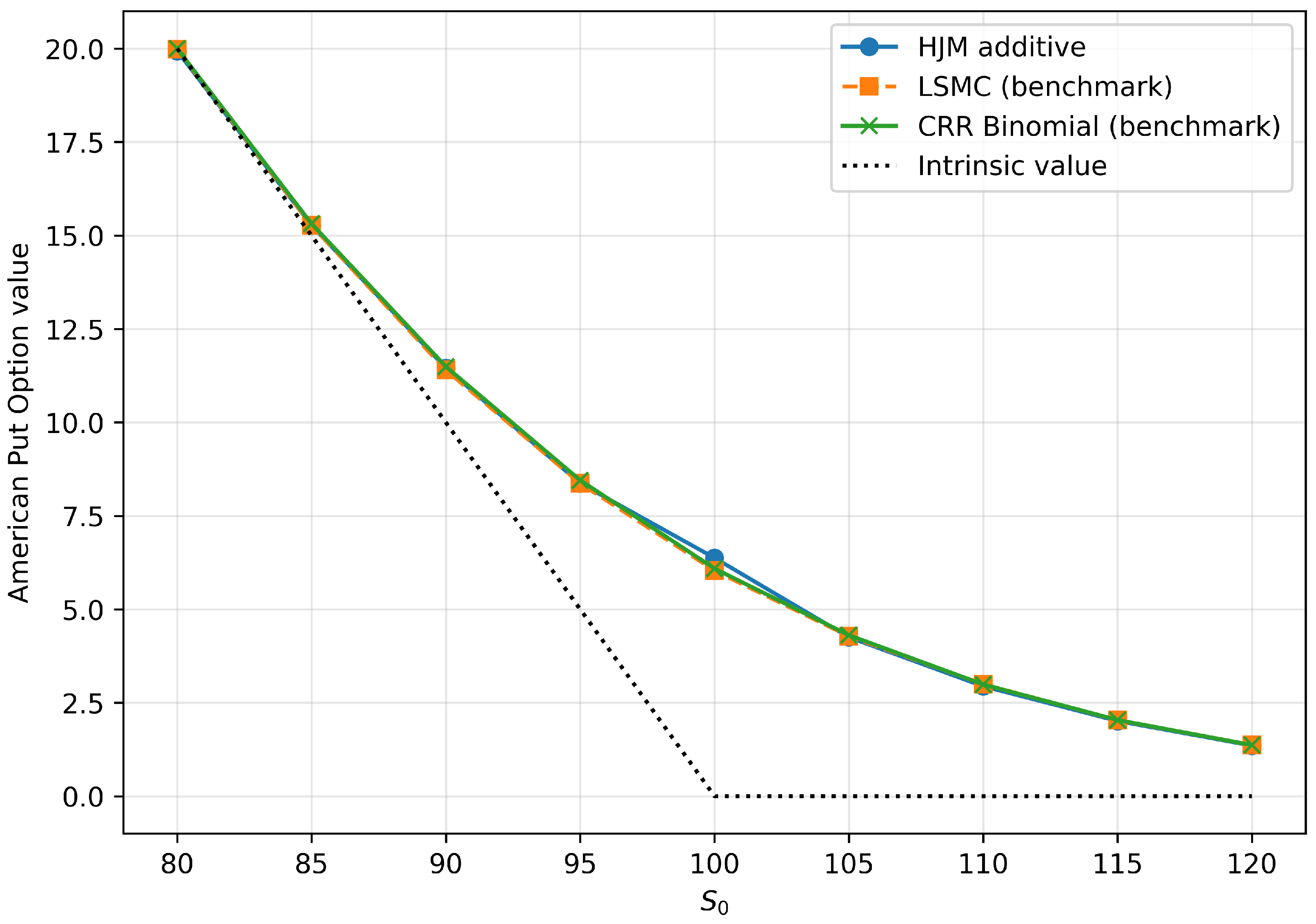
For each value of $S_0$, we simulate $\mathrm{50,000}$ risk-neutral GBM paths using $N=200$ time steps, so the Monte Carlo time increment is $\Delta t=1/200=0.005$. The LSMC algorithm provides an approximate optimal exercise policy and therefore an estimate of the optimal stopping time ${\tau }_0^{*}$ along each simulation path. Using this estimated stopping time, we evaluate the additive representation of the American put option at time zero using Equation (6), and Monte Carlo and Riemann summation. As a benchmark, we compute a CRR binomial American put price using 500 time steps, corresponding to a binomial time increment of $1/500=0.002$. In this way, the binomial price, the LSMC price, and the additive representation price can be compared directly. The implementation of this and other examples in Python 3.12.13 is publicly available.

Table 1. American put prices when $K=100, b=0.20, r=0.05$.

S0	HJM Additive ($\mathit{ϵ}=0.5$)	LSMC	Binomial	|HJM-Bin|	|LSMC-Bin|
80	19.9346	19.9801	20.0000	0.0654	0.0199
85	15.2726	15.2734	15.3150	0.0424	0.0416
90	11.4537	11.4004	11.4922	0.0385	0.0918
95	8.3691	8.3684	8.4510	0.0818	0.0825
100	6.3739	6.0352	6.0888	0.2851	0.0536
105	4.2519	4.2795	4.3066	0.0547	0.0271
110	2.9401	2.9946	2.9884	0.0483	0.0062
115	2.0109	2.0345	2.0376	0.0266	0.0031
120	1.3538	1.3680	1.3672	0.0133	0.0008

and Figure 1 report a numerical comparison of three valuation methods for the American put. Prices are computed for a range of initial stock levels $S_0\in \{80,85,\dots ,120\}$, thereby covering in-the-money, at-the-money, and out-of-the-money cases for the put.

The LSMC estimates track the binomial benchmark very closely across all $S_0$ values. As shown in Table 1, the absolute differences $|V_0^{\mathrm{LSMC}}-V_0^{\mathrm{Bin}}|$ remain on the order of ${10}^{-2}$ to ${10}^{-1}$, with the largest deviation occurring in the deep-in-the-money region. In Figure 1, the LSMC curve (orange) is visually indistinguishable from the binomial curve (green), confirming the reliability of the regression-based continuation value approximation at the simulation scale used.

In the implementation, the drift term ${\mu }_t$ was constructed from the Tanaka decomposition of the put payoff. This is explained in Equation (19), which introduces the local time term ${\displaystyle \frac{1}{2}}d{L}_t^K\left(S\right)$ at the strike K. Since the payoff is not differentiable at $S_t=K$, this term is required in the exact semimartingale decomposition. However, on a discrete simulation grid, the density $d{L}_t^K\left(S\right)/dt$ is singular and cannot be evaluated directly. To obtain a tractable approximation, we replace the Dirac delta at the strike by a Gaussian kernel,

$${\delta }_{\epsilon }(S_t-K)={\displaystyle \frac{1}{\sqrt{2\pi }\epsilon }}exp\left(-{\displaystyle \frac{{(S_t-K)}^2}{2{\epsilon }^2}}\right),$$

where $\epsilon >0$ is a bandwidth parameter. Using the occupation density heuristic for continuous semimartingales, we then approximate the local time density by

$${\displaystyle \frac{d{L}_t^K\left(S\right)}{dt}}\approx b^2{K}^2{\delta }_{\epsilon }(S_t-K).$$

Accordingly, the drift term in the Tanaka decomposition is approximated by

$${\mu }_t\approx -r{S}_t{\mathbf{1}}_{\{S_t<K\}}+{\displaystyle \frac{1}{2}}{b}^2{K}^2{\delta }_{\epsilon }(S_t-K).$$

The main numerical role of the Gaussian kernel method is stabilization. A naive indicator-based approximation would attempt to estimate local time by counting whether the simulated stock lies in a narrow band around the strike. Such estimators can have high variance and can be very sensitive to the chosen bandwidth. By contrast, the Gaussian kernel provides a smooth weighting scheme, so nearby points contribute continuously rather than discontinuously. This reduces simulation noise and produces a more stable approximation of the local time term across paths and time steps. In the reported experiments, the bandwidth parameter is fixed at $\epsilon =0.5$. Smaller values of $\epsilon$ produce a sharper but noisier approximation, whereas larger values provide greater smoothing at the cost of increased bias.

The values obtained from the additive representation also follow the CRR benchmark closely, although with slightly larger discrepancies than LSMC. Table 1 shows that the absolute deviation $|V_0^{\mathrm{HJM}}-V_0^{\mathrm{Bin}}|$ remains moderate (below $0.1$ for most $S_0$) and exhibits systematic behavior across moneyness. In particular, the additive model slightly underprices relative to CRR in the in-the-money region ($S_0=80$–95) and slightly overprices around the at-the-money level ($S_0=100$). This behavior is clearly reflected in Figure 1, where the additive curve (blue) lies just above the benchmark near $S_0=100$.

4.1.2. Example 2

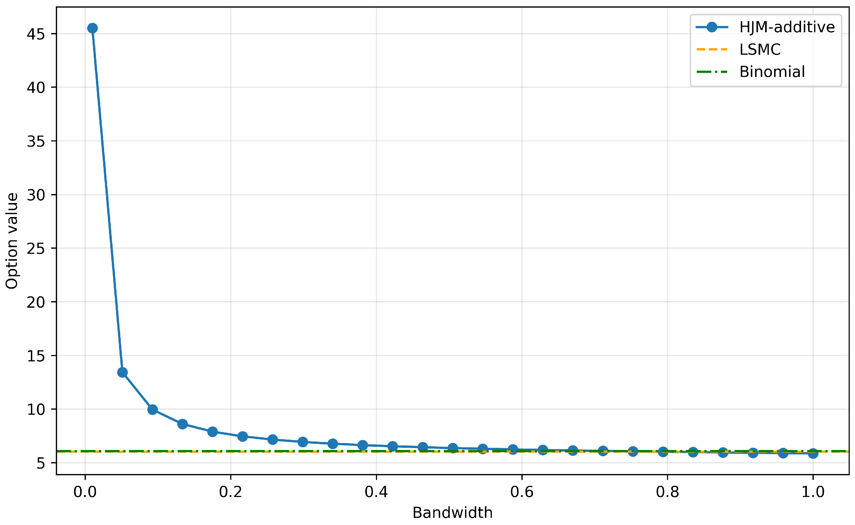
In the previous example, we have set the bandwidth parameter ($\epsilon$) used in the approximation of local time density at $0.5$. To investigate the numerical effect of the bandwidth parameter on the Gaussian kernel approximation used for the local time term, we conduct a bandwidth sensitivity study in the at-the-money case $S_0=100$. All model and simulation parameters are held fixed (i.e $K=100, b=0.20, r=0.05, T=1$), and the same simulated 50,000 stock paths with 200 time steps and LSMC-based stopping rule are used throughout. The only quantity varied is the kernel bandwidth $\epsilon$, which is allowed to range from $0.01$ to $1.00$. For each value of $\epsilon$, we recompute the HJM additive price and compare it with the fixed LSMC and CRR binomial benchmarks. This experiment is designed to isolate the impact of the smoothing parameter in the local time approximation and to evaluate the associated bias-variance trade-off. Results are provided in

Table A1. HJM additive model sensitivity to bandwidth parameter $ϵ$.

Bandwidth $\mathit{ϵ}$	HJM Additive	LSMC	Binomial	|HJM-Bin|	|HJM-LSMC|
0.0100	45.5007	6.0352	6.0888	39.4118	39.4655
0.0512	13.4336	6.0352	6.0888	7.3448	7.3984
0.0925	9.9490	6.0352	6.0888	3.8602	3.9139
0.1338	8.6071	6.0352	6.0888	2.5183	2.5719
0.1750	7.8977	6.0352	6.0888	1.8089	1.8625
0.2163	7.4568	6.0352	6.0888	1.3680	1.4216
0.2575	7.1569	6.0352	6.0888	1.0681	1.1218
0.2988	6.9382	6.0352	6.0888	0.8494	0.9030
0.3400	6.7717	6.0352	6.0888	0.6829	0.7365
0.3813	6.6395	6.0352	6.0888	0.5507	0.6043
0.4225	6.5319	6.0352	6.0888	0.4431	0.4967
0.4638	6.4418	6.0352	6.0888	0.3530	0.4066
0.5050	6.3652	6.0352	6.0888	0.2764	0.3300
0.5462	6.2987	6.0352	6.0888	0.2099	0.2635
0.5875	6.2400	6.0352	6.0888	0.1512	0.2048
0.6288	6.1876	6.0352	6.0888	0.0988	0.1525
0.6700	6.1405	6.0352	6.0888	0.0517	0.1053
0.7113	6.0974	6.0352	6.0888	0.0086	0.0622
0.7525	6.0578	6.0352	6.0888	0.0310	0.0226
0.7938	6.0209	6.0352	6.0888	0.0679	0.0142
0.8350	5.9866	6.0352	6.0888	0.1022	0.0486
0.8762	5.9543	6.0352	6.0888	0.1345	0.0809
0.9175	5.9237	6.0352	6.0888	0.1651	0.1115
0.9588	5.8945	6.0352	6.0888	0.1943	0.1406
1.0000	5.8668	6.0352	6.0888	0.2220	0.1684

and Figure A1.

The results show that the HJM additive price is highly sensitive to the bandwidth when $\epsilon$ is very small, but becomes much more stable once the bandwidth enters a moderate range. For extremely small values of $\epsilon$, the HJM additive price is dramatically inflated relative to both the LSMC and binomial benchmarks. This behavior is consistent with the fact that a very narrow Gaussian kernel produces a sharply peaked approximation to the local time density, so that a small number of simulated path points lying near the strike generate disproportionately large contributions to the Tanaka-based drift term. As a result, the local time correction becomes numerically unstable and introduces a substantial upward bias into the additive price. As the bandwidth increases, the kernel becomes less concentrated and the HJM additive price falls rapidly toward the benchmark level. This indicates that the extreme overpricing observed at very small bandwidths is primarily a variance effect caused by undersmoothing. Once the bandwidth becomes moderate, approximately in the range $0.4$ to $1.0$ in this experiment, the HJM additive price stabilizes and lies much closer to the LSMC and binomial values. In that region, the smoothing is sufficient to regularize the local time contribution without allowing it to dominate the entire pricing integral.

4.1.3. Example 3

The first numerical experiment is intended as a proof of concept for the additive representation under a single baseline specification, with fixed maturity and volatility and a moderate grid of initial stock prices. Its role is to demonstrate that the additive HJM-based valuation can be implemented numerically and produces prices close to standard benchmarks such as LSMC and the CRR binomial tree. By itself, however, that experiment is too narrow to assess robustness. Since American put valuation is sensitive to moneyness, maturity, and volatility, an agreement observed under one parameter choice may not persist across broader market conditions. For this reason, we perform a second, expanded experiment in which the same option type is studied over a larger grid of stock prices, maturities, and volatilities. This experiment is designed not merely to illustrate feasibility, but to evaluate the stability of the additive representation across in-the-money, at-the-money, and out-of-the-money configurations, as well as under short- and long-dated contracts and under low- and high-volatility regimes. In this sense, the first experiment provides an initial illustration, while this experiment provides a broader robustness check.

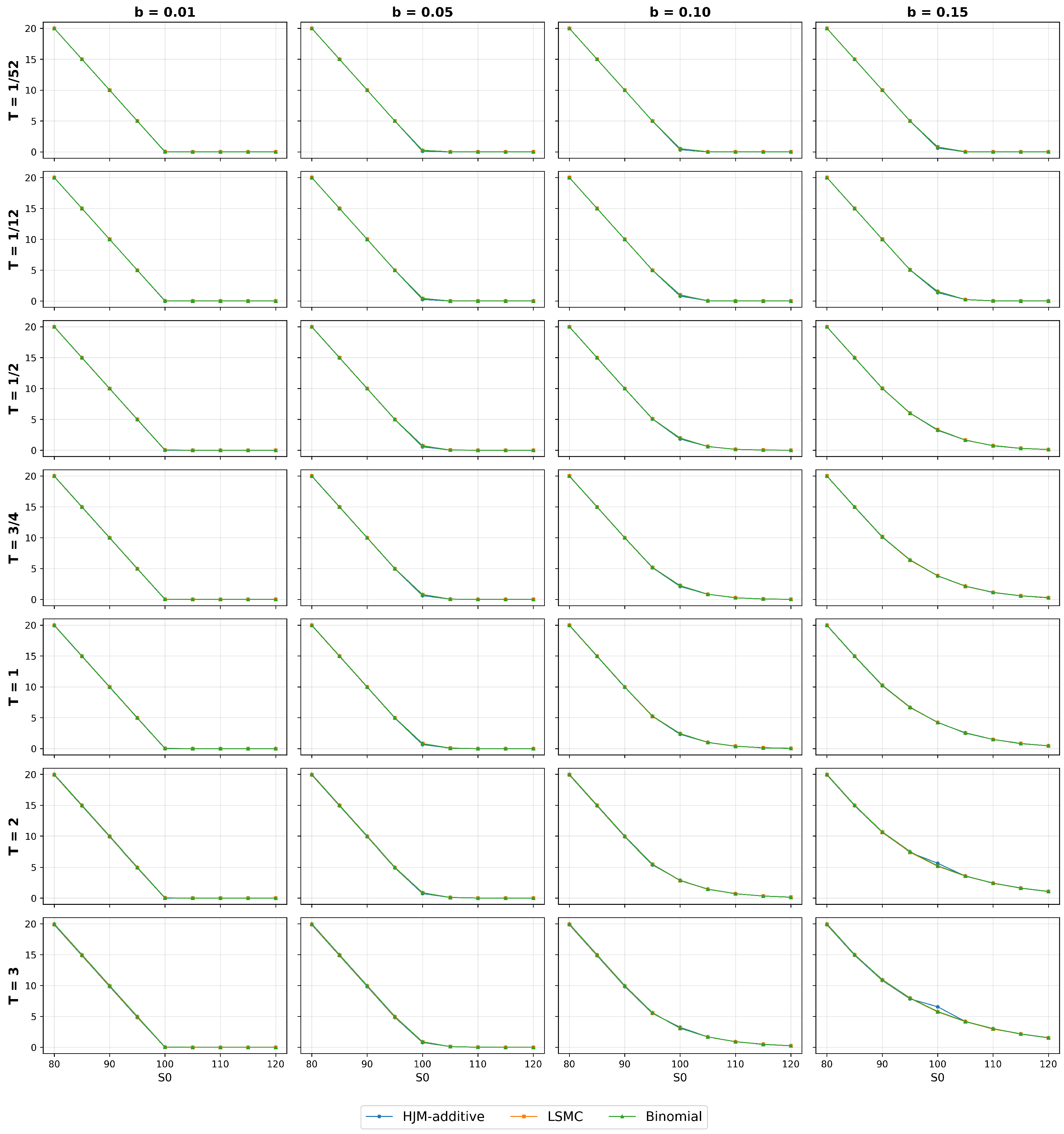
This experiment keeps the same option type as in Example 1, namely American put with strike price $K=100, r=0.05$, but broadens the other parameter space substantially by considering a grid of initial stock prices $S_0\in \{80,85,90,95,100,105,110,115,120\}$, maturities $T\in \{1/52,1/12,6/12,9/12,1,2,3\}$, and stock volatility $b\in \{0.01,0.05,0.1,0.15,0.2,0.3,$$0.5,1.0\}$. This creates a much richer family of contracts spanning deep in-the-money, near-the-money, and out-of-the-money cases, as well as short, medium, and long-dated maturities under low and high-volatility environments. The purpose is no longer just to show that the method works in one example, but to assess its robustness across a systematic range of economically relevant scenarios.

For each parameter combination, three prices were computed and compared. First, the CRR binomial tree with 500 time steps was used as the benchmark valuation method. Second, LSMC implementation was used to approximate the American put value and, importantly, to estimate the optimal exercise policy along simulated paths. Third, the additive HJM-based price was evaluated using the representation developed earlier in the paper. In that computation, the stock price paths were simulated under the risk-neutral geometric Brownian motion, the stopping times were taken from the LSMC exercise rule, and the drift term in the additive representation was approximated using the Tanaka-based decomposition of the gain process. The local time contribution was incorporated through a Gaussian kernel approximation with bandwidth 0.50. The Monte Carlo simulation used 50,000 paths and 200 time steps for each case.

The numerical procedure was therefore designed to isolate the performance of the additive representation itself rather than to solve the stopping problem independently. The LSMC method provided an approximate exercise strategy, while the additive formula translated that strategy into a forward-drift-based valuation. Comparing the resulting HJM additive prices against both LSMC and the CRR benchmark allows one to assess whether the forward representation remains accurate across a wide range of market conditions. The inclusion of multiple moneyness categories is particularly important because the early exercise feature of an American put is most pronounced in the in-the-money region, whereas the out-of-the-money region provides a useful test of the model when continuation value dominates intrinsic value. Similarly, varying maturity and volatility tests the sensitivity of the representation to both time value and dispersion in the underlying stock process.

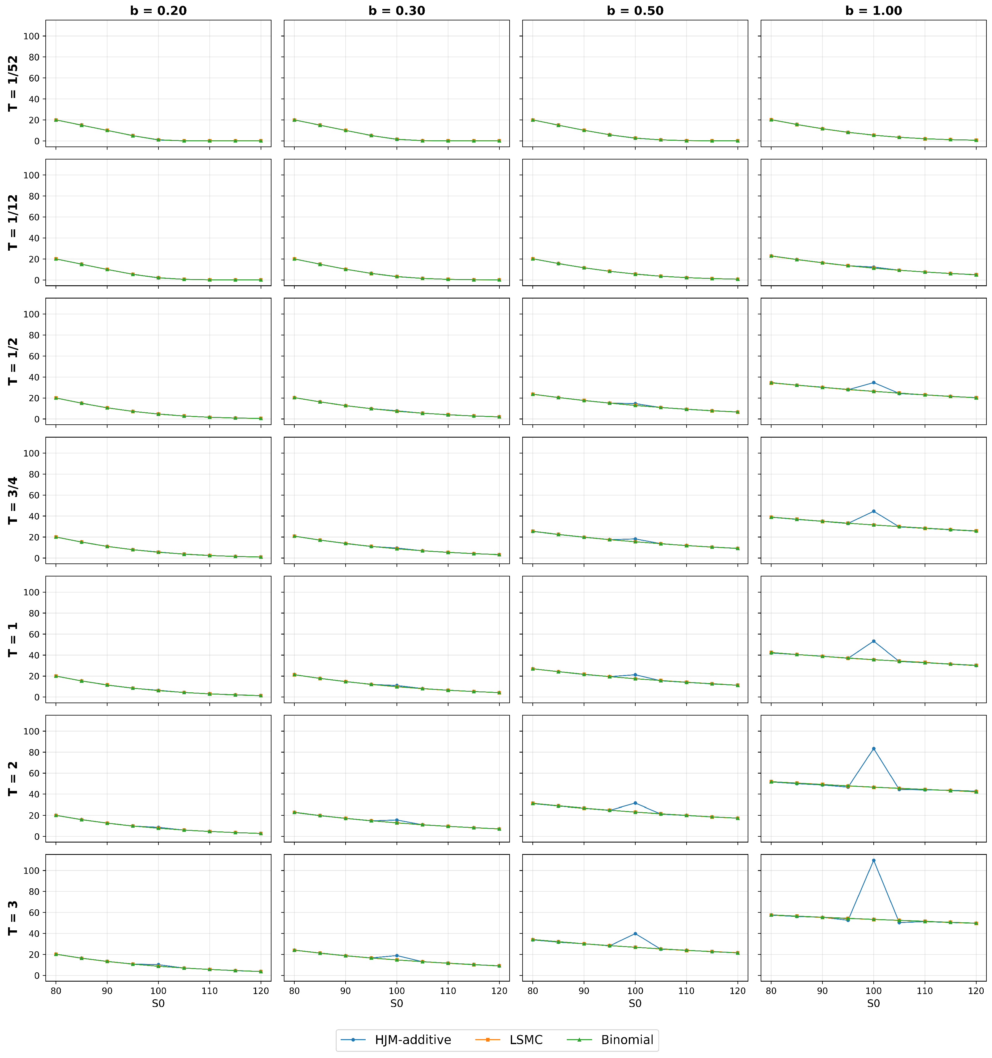
To summarize the results, we report the full pricing table for all parameter combinations, including moneyness, in

Table A2. Extended American put pricing experiment comparing the HJM additive representation, LSMC, and CRR binomial benchmark across moneyness, maturity, and volatility.

Moneyness	${\mathit{S}}_0$	T	b	HJM	LSMC	Binomial	|HJM-Bin|	|LSMC-Bin|
ITM	80.0	0.0192	0.01	19.9990	19.9995	20.0000	0.0010	0.0005
ITM	85.0	0.0192	0.01	14.9990	14.9996	15.0000	0.0010	0.0004
ITM	90.0	0.0192	0.01	9.9990	9.9995	10.0000	0.0010	0.0005
ITM	95.0	0.0192	0.01	4.9990	4.9995	5.0000	0.0010	0.0005
ATM	100.0	0.0192	0.01	−0.0097	0.0290	0.0290	0.0387	0.0001
OTM	105.0	0.0192	0.01	0.0000	0.0000	0.0000	0.0000	0.0000
OTM	110.0	0.0192	0.01	0.0000	0.0000	0.0000	0.0000	0.0000
OTM	115.0	0.0192	0.01	0.0000	0.0000	0.0000	0.0000	0.0000
OTM	120.0	0.0192	0.01	0.0000	0.0000	0.0000	0.0000	0.0000
ITM	80.0	0.0833	0.01	19.9958	19.9979	20.0000	0.0042	0.0021
ITM	85.0	0.0833	0.01	14.9958	14.9980	15.0000	0.0042	0.0020
ITM	90.0	0.0833	0.01	9.9958	9.9979	10.0000	0.0042	0.0021
ITM	95.0	0.0833	0.01	4.9958	4.9979	5.0000	0.0042	0.0021
ATM	100.0	0.0833	0.01	−0.0082	0.0347	0.0355	0.0437	0.0008
OTM	105.0	0.0833	0.01	0.0000	0.0000	0.0000	0.0000	0.0000
OTM	110.0	0.0833	0.01	0.0000	0.0000	0.0000	0.0000	0.0000
OTM	115.0	0.0833	0.01	0.0000	0.0000	0.0000	0.0000	0.0000
OTM	120.0	0.0833	0.01	0.0000	0.0000	0.0000	0.0000	0.0000
ITM	80.0	0.5000	0.01	19.9750	19.9872	20.0000	0.0250	0.0128
ITM	85.0	0.5000	0.01	14.9750	14.9874	15.0000	0.0250	0.0126
ITM	90.0	0.5000	0.01	9.9750	9.9873	10.0000	0.0250	0.0127
ITM	95.0	0.5000	0.01	4.9750	4.9876	5.0000	0.0250	0.0124
ATM	100.0	0.5000	0.01	0.0059	0.0353	0.0364	0.0305	0.0011
OTM	105.0	0.5000	0.01	0.0000	0.0000	0.0000	0.0000	0.0000
OTM	110.0	0.5000	0.01	0.0000	0.0000	0.0000	0.0000	0.0000
OTM	115.0	0.5000	0.01	0.0000	0.0000	0.0000	0.0000	0.0000
OTM	120.0	0.5000	0.01	0.0000	0.0000	0.0000	0.0000	0.0000
ITM	80.0	0.7500	0.01	19.9625	19.9814	20.0000	0.0375	0.0186
ITM	85.0	0.7500	0.01	14.9625	14.9813	15.0000	0.0375	0.0187
ITM	90.0	0.7500	0.01	9.9625	9.9812	10.0000	0.0375	0.0188
ITM	95.0	0.7500	0.01	4.9625	4.9813	5.0000	0.0375	0.0187
ATM	100.0	0.7500	0.01	0.0060	0.0353	0.0358	0.0298	0.0005
OTM	105.0	0.7500	0.01	0.0000	0.0000	0.0000	0.0000	0.0000
OTM	110.0	0.7500	0.01	0.0000	0.0000	0.0000	0.0000	0.0000
OTM	115.0	0.7500	0.01	0.0000	0.0000	0.0000	0.0000	0.0000
OTM	120.0	0.7500	0.01	0.0000	0.0000	0.0000	0.0000	0.0000
ITM	80.0	1.0000	0.01	19.9500	19.9752	20.0000	0.0500	0.0248
ITM	85.0	1.0000	0.01	14.9500	14.9750	15.0000	0.0500	0.0250
ITM	90.0	1.0000	0.01	9.9500	9.9748	10.0000	0.0500	0.0252
ITM	95.0	1.0000	0.01	4.9500	4.9745	5.0000	0.0500	0.0255
ATM	100.0	1.0000	0.01	0.0066	0.0344	0.0360	0.0294	0.0016
OTM	105.0	1.0000	0.01	0.0000	0.0000	0.0000	0.0000	0.0000
OTM	110.0	1.0000	0.01	0.0000	0.0000	0.0000	0.0000	0.0000
OTM	115.0	1.0000	0.01	0.0000	0.0000	0.0000	0.0000	0.0000
OTM	120.0	1.0000	0.01	0.0000	0.0000	0.0000	0.0000	0.0000
ITM	80.0	2.0000	0.01	19.9000	19.9496	20.0000	0.1000	0.0504
ITM	85.0	2.0000	0.01	14.9000	14.9502	15.0000	0.1000	0.0498
ITM	90.0	2.0000	0.01	9.9000	9.9494	10.0000	0.1000	0.0506
ITM	95.0	2.0000	0.01	4.9000	4.9500	5.0000	0.1000	0.0500
ATM	100.0	2.0000	0.01	0.0065	0.0325	0.0341	0.0277	0.0016
OTM	105.0	2.0000	0.01	0.0000	0.0000	0.0000	0.0000	0.0000
OTM	110.0	2.0000	0.01	0.0000	0.0000	0.0000	0.0000	0.0000
OTM	115.0	2.0000	0.01	0.0000	0.0000	0.0000	0.0000	0.0000
OTM	120.0	2.0000	0.01	0.0000	0.0000	0.0000	0.0000	0.0000
ITM	80.0	3.0000	0.01	19.8501	19.9251	20.0000	0.1499	0.0749
ITM	85.0	3.0000	0.01	14.8501	14.9259	15.0000	0.1499	0.0741
ITM	90.0	3.0000	0.01	9.8501	9.9243	10.0000	0.1499	0.0757
ITM	95.0	3.0000	0.01	4.8501	4.9251	5.0000	0.1499	0.0749
ATM	100.0	3.0000	0.01	0.0067	0.0303	0.0342	0.0274	0.0039
OTM	105.0	3.0000	0.01	0.0000	0.0000	0.0000	0.0000	0.0000
OTM	110.0	3.0000	0.01	0.0000	0.0000	0.0000	0.0000	0.0000
OTM	115.0	3.0000	0.01	0.0000	0.0000	0.0000	0.0000	0.0000
OTM	120.0	3.0000	0.01	0.0000	0.0000	0.0000	0.0000	0.0000
ITM	80.0	0.0192	0.05	19.9990	19.9995	20.0000	0.0010	0.0005
ITM	85.0	0.0192	0.05	14.9990	14.9995	15.0000	0.0010	0.0005
ITM	90.0	0.0192	0.05	9.9990	9.9996	10.0000	0.0010	0.0004
ITM	95.0	0.0192	0.05	4.9990	4.9998	5.0000	0.0010	0.0002
ATM	100.0	0.0192	0.05	0.0973	0.2372	0.2389	0.1416	0.0017
OTM	105.0	0.0192	0.05	0.0000	0.0000	0.0000	0.0000	0.0000
OTM	110.0	0.0192	0.05	0.0000	0.0000	0.0000	0.0000	0.0000
OTM	115.0	0.0192	0.05	0.0000	0.0000	0.0000	0.0000	0.0000
OTM	120.0	0.0192	0.05	0.0000	0.0000	0.0000	0.0000	0.0000
ITM	80.0	0.0833	0.05	19.9958	19.9979	20.0000	0.0042	0.0021
ITM	85.0	0.0833	0.05	14.9958	14.9978	15.0000	0.0042	0.0022
ITM	90.0	0.0833	0.05	9.9958	9.9980	10.0000	0.0042	0.0020
ITM	95.0	0.0833	0.05	4.9958	4.9983	5.0000	0.0042	0.0017
ATM	100.0	0.0833	0.05	0.2591	0.4286	0.4298	0.1707	0.0012
OTM	105.0	0.0833	0.05	0.0001	0.0001	0.0000	0.0001	0.0000
OTM	110.0	0.0833	0.05	0.0000	0.0000	0.0000	0.0000	0.0000
OTM	115.0	0.0833	0.05	0.0000	0.0000	0.0000	0.0000	0.0000
OTM	120.0	0.0833	0.05	0.0000	0.0000	0.0000	0.0000	0.0000
ITM	80.0	0.5000	0.05	19.9750	19.9888	20.0000	0.0250	0.0112
ITM	85.0	0.5000	0.05	14.9750	14.9867	15.0000	0.0250	0.0133
ITM	90.0	0.5000	0.05	9.9750	9.9870	10.0000	0.0250	0.0130
ITM	95.0	0.5000	0.05	4.9750	4.9869	5.0000	0.0250	0.0131
ATM	100.0	0.5000	0.05	0.5546	0.7206	0.7290	0.1743	0.0084
OTM	105.0	0.5000	0.05	0.0316	0.0287	0.0291	0.0025	0.0004
OTM	110.0	0.5000	0.05	0.0004	0.0006	0.0003	0.0000	0.0002
OTM	115.0	0.5000	0.05	0.0000	0.0000	0.0000	0.0000	0.0000
OTM	120.0	0.5000	0.05	0.0000	0.0000	0.0000	0.0000	0.0000
ITM	80.0	0.7500	0.05	19.9625	19.9797	20.0000	0.0375	0.0203
ITM	85.0	0.7500	0.05	14.9625	14.9813	15.0000	0.0375	0.0187
ITM	90.0	0.7500	0.05	9.9625	9.9803	10.0000	0.0375	0.0197
ITM	95.0	0.7500	0.05	4.9625	4.9812	5.0000	0.0375	0.0188
ATM	100.0	0.7500	0.05	0.6120	0.7858	0.7870	0.1750	0.0012
OTM	105.0	0.7500	0.05	0.0533	0.0497	0.0509	0.0024	0.0011
OTM	110.0	0.7500	0.05	0.0013	0.0020	0.0016	0.0003	0.0004
OTM	115.0	0.7500	0.05	0.0000	0.0000	0.0000	0.0000	0.0000
OTM	120.0	0.7500	0.05	0.0000	0.0000	0.0000	0.0000	0.0000
ITM	80.0	1.0000	0.05	19.9500	19.9763	20.0000	0.0500	0.0237
ITM	85.0	1.0000	0.05	14.9500	14.9745	15.0000	0.0500	0.0255
ITM	90.0	1.0000	0.05	9.9500	9.9736	10.0000	0.0500	0.0264
ITM	95.0	1.0000	0.05	4.9500	4.9775	5.0000	0.0500	0.0225
ATM	100.0	1.0000	0.05	0.6551	0.8171	0.8220	0.1669	0.0049
OTM	105.0	1.0000	0.05	0.0713	0.0685	0.0680	0.0033	0.0004
OTM	110.0	1.0000	0.05	0.0034	0.0040	0.0035	0.0001	0.0005
OTM	115.0	1.0000	0.05	0.0001	0.0001	0.0001	0.0000	0.0000
OTM	120.0	1.0000	0.05	0.0000	0.0000	0.0000	0.0000	0.0000
ITM	80.0	2.0000	0.05	19.9000	19.9493	20.0000	0.1000	0.0507
ITM	85.0	2.0000	0.05	14.9000	14.9518	15.0000	0.1000	0.0482
ITM	90.0	2.0000	0.05	9.9000	9.9510	10.0000	0.1000	0.0490
ITM	95.0	2.0000	0.05	4.9000	4.9513	5.0000	0.1000	0.0487
ATM	100.0	2.0000	0.05	0.7438	0.8681	0.8783	0.1345	0.0102
OTM	105.0	2.0000	0.05	0.1085	0.1043	0.1050	0.0035	0.0007
OTM	110.0	2.0000	0.05	0.0112	0.0121	0.0112	0.0000	0.0009
OTM	115.0	2.0000	0.05	0.0008	0.0016	0.0010	0.0002	0.0006
OTM	120.0	2.0000	0.05	0.0001	0.0002	0.0001	0.0000	0.0002
ITM	80.0	3.0000	0.05	19.8501	19.9241	20.0000	0.1499	0.0759
ITM	85.0	3.0000	0.05	14.8501	14.9234	15.0000	0.1499	0.0766
ITM	90.0	3.0000	0.05	9.8501	9.9302	10.0000	0.1499	0.0698
ITM	95.0	3.0000	0.05	4.8501	4.9261	5.0000	0.1499	0.0739
ATM	100.0	3.0000	0.05	0.7861	0.8808	0.8947	0.1086	0.0139
OTM	105.0	3.0000	0.05	0.1222	0.1164	0.1182	0.0040	0.0019
OTM	110.0	3.0000	0.05	0.0154	0.0155	0.0156	0.0001	0.0000
OTM	115.0	3.0000	0.05	0.0020	0.0026	0.0020	0.0000	0.0007
OTM	120.0	3.0000	0.05	0.0002	0.0006	0.0002	0.0001	0.0004
ITM	80.0	0.0192	0.10	19.9990	19.9986	20.0000	0.0010	0.0014
ITM	85.0	0.0192	0.10	14.9983	15.0009	15.0000	0.0017	0.0009
ITM	90.0	0.0192	0.10	9.9981	9.9999	10.0000	0.0019	0.0001
ITM	95.0	0.0192	0.10	4.9988	5.0000	5.0000	0.0012	0.0000
ATM	100.0	0.0192	0.10	0.3423	0.5047	0.5128	0.1706	0.0082
OTM	105.0	0.0192	0.10	0.0001	0.0001	0.0001	0.0001	0.0000
OTM	110.0	0.0192	0.10	0.0000	0.0000	0.0000	0.0000	0.0000
OTM	115.0	0.0192	0.10	0.0000	0.0000	0.0000	0.0000	0.0000
OTM	120.0	0.0192	0.10	0.0000	0.0000	0.0000	0.0000	0.0000
ITM	80.0	0.0833	0.10	19.9958	19.9962	20.0000	0.0042	0.0038
ITM	85.0	0.0833	0.10	14.9957	14.9970	15.0000	0.0043	0.0030
ITM	90.0	0.0833	0.10	9.9958	9.9978	10.0000	0.0042	0.0022
ITM	95.0	0.0833	0.10	4.9949	5.0009	5.0000	0.0051	0.0009
ATM	100.0	0.0833	0.10	0.8071	0.9902	0.9880	0.1809	0.0021
OTM	105.0	0.0833	0.10	0.0425	0.0410	0.0392	0.0032	0.0017
OTM	110.0	0.0833	0.10	0.0002	0.0004	0.0002	0.0000	0.0002
OTM	115.0	0.0833	0.10	0.0000	0.0000	0.0000	0.0000	0.0000
OTM	120.0	0.0833	0.10	0.0000	0.0000	0.0000	0.0000	0.0000
ITM	80.0	0.5000	0.10	19.9750	19.9883	20.0000	0.0250	0.0117
ITM	85.0	0.5000	0.10	14.9750	14.9883	15.0000	0.0250	0.0117
ITM	90.0	0.5000	0.10	9.9750	9.9892	10.0000	0.0250	0.0108
ITM	95.0	0.5000	0.10	5.0690	5.0892	5.0931	0.0240	0.0038
ATM	100.0	0.5000	0.10	1.8164	1.9509	1.9722	0.1558	0.0213
OTM	105.0	0.5000	0.10	0.6050	0.6056	0.6036	0.0015	0.0020
OTM	110.0	0.5000	0.10	0.1428	0.1464	0.1430	0.0002	0.0035
OTM	115.0	0.5000	0.10	0.0274	0.0283	0.0264	0.0010	0.0019
OTM	120.0	0.5000	0.10	0.0029	0.0045	0.0038	0.0010	0.0007
ITM	80.0	0.7500	0.10	19.9625	19.9826	20.0000	0.0375	0.0174
ITM	85.0	0.7500	0.10	14.9625	14.9836	15.0000	0.0375	0.0164
ITM	90.0	0.7500	0.10	9.9624	9.9781	10.0000	0.0376	0.0219
ITM	95.0	0.7500	0.10	5.1523	5.1763	5.1897	0.0374	0.0134
ATM	100.0	0.7500	0.10	2.1031	2.2311	2.2426	0.1396	0.0115
OTM	105.0	0.7500	0.10	0.8333	0.8398	0.8391	0.0058	0.0008
OTM	110.0	0.7500	0.10	0.2707	0.2741	0.2692	0.0015	0.0049
OTM	115.0	0.7500	0.10	0.0725	0.0736	0.0740	0.0015	0.0004
OTM	120.0	0.7500	0.10	0.0180	0.0190	0.0177	0.0002	0.0013
ITM	80.0	1.0000	0.10	19.9500	19.9729	20.0000	0.0500	0.0271
ITM	85.0	1.0000	0.10	14.9500	14.9753	15.0000	0.0500	0.0247
ITM	90.0	1.0000	0.10	9.9500	9.9792	10.0000	0.0500	0.0208
ITM	95.0	1.0000	0.10	5.2327	5.2265	5.2724	0.0397	0.0458
ATM	100.0	1.0000	0.10	2.3215	2.4377	2.4360	0.1145	0.0017
OTM	105.0	1.0000	0.10	1.0055	0.9916	1.0202	0.0148	0.0287
OTM	110.0	1.0000	0.10	0.3776	0.3883	0.3846	0.0070	0.0037
OTM	115.0	1.0000	0.10	0.1247	0.1265	0.1307	0.0060	0.0042
OTM	120.0	1.0000	0.10	0.0403	0.0422	0.0402	0.0000	0.0020
ITM	80.0	2.0000	0.10	19.9000	19.9505	20.0000	0.1000	0.0495
ITM	85.0	2.0000	0.10	14.9000	14.9534	15.0000	0.1000	0.0466
ITM	90.0	2.0000	0.10	9.9000	9.9511	10.0000	0.1000	0.0489
ITM	95.0	2.0000	0.10	5.3892	5.4758	5.4920	0.1029	0.0162
ATM	100.0	2.0000	0.10	2.8926	2.8360	2.8755	0.0172	0.0394
OTM	105.0	2.0000	0.10	1.4327	1.4418	1.4605	0.0278	0.0188
OTM	110.0	2.0000	0.10	0.7170	0.7194	0.7173	0.0003	0.0021
OTM	115.0	2.0000	0.10	0.3390	0.3402	0.3394	0.0004	0.0008
OTM	120.0	2.0000	0.10	0.1463	0.1546	0.1558	0.0094	0.0011
ITM	80.0	3.0000	0.10	19.8501	19.9236	20.0000	0.1499	0.0764
ITM	85.0	3.0000	0.10	14.8501	14.9273	15.0000	0.1499	0.0727
ITM	90.0	3.0000	0.10	9.8501	9.9158	10.0000	0.1499	0.0842
ITM	95.0	3.0000	0.10	5.4970	5.5756	5.6109	0.1139	0.0352
ATM	100.0	3.0000	0.10	3.2445	3.0950	3.0922	0.1523	0.0028
OTM	105.0	3.0000	0.10	1.6799	1.6789	1.6904	0.0105	0.0115
OTM	110.0	3.0000	0.10	0.9061	0.9066	0.9139	0.0078	0.0073
OTM	115.0	3.0000	0.10	0.4724	0.4861	0.4874	0.0150	0.0013
OTM	120.0	3.0000	0.10	0.2496	0.2582	0.2569	0.0073	0.0013
ITM	80.0	0.0192	0.15	19.9983	19.9995	20.0000	0.0017	0.0005
ITM	85.0	0.0192	0.15	14.9988	14.9999	15.0000	0.0012	0.0001
ITM	90.0	0.0192	0.15	9.9989	9.9992	10.0000	0.0011	0.0008
ITM	95.0	0.0192	0.15	4.9983	5.0005	5.0000	0.0017	0.0005
ATM	100.0	0.0192	0.15	0.6112	0.7901	0.7882	0.1770	0.0019
OTM	105.0	0.0192	0.15	0.0068	0.0056	0.0059	0.0009	0.0003
OTM	110.0	0.0192	0.15	0.0000	0.0000	0.0000	0.0000	0.0000
OTM	115.0	0.0192	0.15	0.0000	0.0000	0.0000	0.0000	0.0000
OTM	120.0	0.0192	0.15	0.0000	0.0000	0.0000	0.0000	0.0000
ITM	80.0	0.0833	0.15	19.9953	19.9981	20.0000	0.0047	0.0019
ITM	85.0	0.0833	0.15	14.9953	14.9987	15.0000	0.0047	0.0013
ITM	90.0	0.0833	0.15	9.9958	9.9980	10.0000	0.0042	0.0020
ITM	95.0	0.0833	0.15	5.0544	5.0564	5.0638	0.0094	0.0074
ATM	100.0	0.0833	0.15	1.3669	1.5480	1.5557	0.1888	0.0077
OTM	105.0	0.0833	0.15	0.2432	0.2374	0.2403	0.0029	0.0028
OTM	110.0	0.0833	0.15	0.0177	0.0176	0.0168	0.0008	0.0007
OTM	115.0	0.0833	0.15	0.0005	0.0006	0.0005	0.0000	0.0001
OTM	120.0	0.0833	0.15	0.0000	0.0000	0.0000	0.0000	0.0000
ITM	80.0	0.5000	0.15	19.9750	19.9918	20.0000	0.0250	0.0082
ITM	85.0	0.5000	0.15	14.9750	14.9830	15.0000	0.0250	0.0170
ITM	90.0	0.5000	0.15	10.0041	10.0346	10.0330	0.0289	0.0016
ITM	95.0	0.5000	0.15	6.0159	5.9795	6.0258	0.0099	0.0463
ATM	100.0	0.5000	0.15	3.2275	3.3212	3.2997	0.0723	0.0215
OTM	105.0	0.5000	0.15	1.6500	1.6469	1.6404	0.0096	0.0065
OTM	110.0	0.5000	0.15	0.7265	0.7448	0.7386	0.0120	0.0062
OTM	115.0	0.5000	0.15	0.3004	0.3143	0.3033	0.0030	0.0110
OTM	120.0	0.5000	0.15	0.1138	0.1154	0.1136	0.0002	0.0018
ITM	80.0	0.7500	0.15	19.9625	19.9846	20.0000	0.0375	0.0154
ITM	85.0	0.7500	0.15	14.9615	14.9818	15.0000	0.0385	0.0182
ITM	90.0	0.7500	0.15	10.0978	10.1417	10.1431	0.0453	0.0014
ITM	95.0	0.7500	0.15	6.3616	6.3362	6.4171	0.0555	0.0810
ATM	100.0	0.7500	0.15	3.8159	3.8342	3.8313	0.0154	0.0029
OTM	105.0	0.7500	0.15	2.1280	2.1192	2.1580	0.0300	0.0389
OTM	110.0	0.7500	0.15	1.1218	1.1461	1.1461	0.0243	0.0000
OTM	115.0	0.7500	0.15	0.5726	0.5872	0.5746	0.0020	0.0125
OTM	120.0	0.7500	0.15	0.2671	0.2831	0.2744	0.0073	0.0087
ITM	80.0	1.0000	0.15	19.9500	19.9779	20.0000	0.0500	0.0221
ITM	85.0	1.0000	0.15	14.9495	14.9720	15.0000	0.0505	0.0280
ITM	90.0	1.0000	0.15	10.2029	10.2401	10.2661	0.0632	0.0260
ITM	95.0	1.0000	0.15	6.6559	6.6586	6.7235	0.0675	0.0648
ATM	100.0	1.0000	0.15	4.2624	4.2351	4.2315	0.0309	0.0036
OTM	105.0	1.0000	0.15	2.5108	2.5543	2.5611	0.0503	0.0068
OTM	110.0	1.0000	0.15	1.4893	1.4864	1.4874	0.0019	0.0010
OTM	115.0	1.0000	0.15	0.8036	0.8272	0.8338	0.0302	0.0066
OTM	120.0	1.0000	0.15	0.4492	0.4472	0.4508	0.0016	0.0036
ITM	80.0	2.0000	0.15	19.8991	19.9488	20.0000	0.1009	0.0512
ITM	85.0	2.0000	0.15	14.9144	14.9583	15.0000	0.0856	0.0417
ITM	90.0	2.0000	0.15	10.5848	10.6124	10.6818	0.0969	0.0693
ITM	95.0	2.0000	0.15	7.4028	7.4256	7.5226	0.1198	0.0971
ATM	100.0	2.0000	0.15	5.6510	5.1623	5.2316	0.4194	0.0693
OTM	105.0	2.0000	0.15	3.5629	3.5668	3.5968	0.0339	0.0300
OTM	110.0	2.0000	0.15	2.4092	2.4175	2.4383	0.0291	0.0209
OTM	115.0	2.0000	0.15	1.6081	1.6131	1.6372	0.0290	0.0241
OTM	120.0	2.0000	0.15	1.0662	1.0923	1.0863	0.0202	0.0059
ITM	80.0	3.0000	0.15	19.8501	19.9349	20.0000	0.1499	0.0651
ITM	85.0	3.0000	0.15	14.9099	14.9934	15.0247	0.1148	0.0313
ITM	90.0	3.0000	0.15	10.8229	10.9063	10.9656	0.1426	0.0593
ITM	95.0	3.0000	0.15	7.8550	7.9450	7.9881	0.1331	0.0430
ATM	100.0	3.0000	0.15	6.5648	5.7287	5.7993	0.7656	0.0705
OTM	105.0	3.0000	0.15	4.1824	4.1572	4.1968	0.0145	0.0397
OTM	110.0	3.0000	0.15	3.0229	2.9566	3.0254	0.0025	0.0687
OTM	115.0	3.0000	0.15	2.1523	2.1710	2.1721	0.0199	0.0012
OTM	120.0	3.0000	0.15	1.5260	1.5357	1.5556	0.0295	0.0198
ITM	80.0	0.0192	0.20	19.9980	20.0005	20.0000	0.0020	0.0005
ITM	85.0	0.0192	0.20	14.9984	14.9994	15.0000	0.0016	0.0006
ITM	90.0	0.0192	0.20	9.9990	9.9990	10.0000	0.0010	0.0010
ITM	95.0	0.0192	0.20	5.0016	5.0078	5.0029	0.0012	0.0049
ATM	100.0	0.0192	0.20	0.8798	1.0631	1.0639	0.1841	0.0008
OTM	105.0	0.0192	0.20	0.0438	0.0420	0.0413	0.0025	0.0007
OTM	110.0	0.0192	0.20	0.0002	0.0001	0.0002	0.0000	0.0000
OTM	115.0	0.0192	0.20	0.0000	0.0000	0.0000	0.0000	0.0000
OTM	120.0	0.0192	0.20	0.0000	0.0000	0.0000	0.0000	0.0000
ITM	80.0	0.0833	0.20	19.9939	20.0008	20.0000	0.0061	0.0008
ITM	85.0	0.0833	0.20	14.9936	14.9978	15.0000	0.0064	0.0022
ITM	90.0	0.0833	0.20	9.9926	9.9973	10.0000	0.0074	0.0027
ITM	95.0	0.0833	0.20	5.3372	5.3337	5.3561	0.0189	0.0224
ATM	100.0	0.0833	0.20	1.9606	2.1137	2.1262	0.1656	0.0125
OTM	105.0	0.0833	0.20	0.5804	0.5678	0.5807	0.0003	0.0129
OTM	110.0	0.0833	0.20	0.1058	0.1049	0.1053	0.0005	0.0003
OTM	115.0	0.0833	0.20	0.0116	0.0121	0.0126	0.0010	0.0005
OTM	120.0	0.0833	0.20	0.0010	0.0011	0.0010	0.0001	0.0000
ITM	80.0	0.5000	0.20	19.9701	19.9940	20.0000	0.0299	0.0060
ITM	85.0	0.5000	0.20	14.9943	15.0067	15.0206	0.0263	0.0139
ITM	90.0	0.5000	0.20	10.6199	10.5899	10.6670	0.0470	0.0771
ITM	95.0	0.5000	0.20	7.1732	7.1859	7.2233	0.0501	0.0374
ATM	100.0	0.5000	0.20	4.6915	4.6296	4.6544	0.0371	0.0248
OTM	105.0	0.5000	0.20	2.8297	2.8253	2.8555	0.0258	0.0302
OTM	110.0	0.5000	0.20	1.6526	1.6634	1.6698	0.0172	0.0064
OTM	115.0	0.5000	0.20	0.9188	0.9090	0.9297	0.0109	0.0207
OTM	120.0	0.5000	0.20	0.4875	0.4959	0.4981	0.0106	0.0022
ITM	80.0	0.7500	0.20	19.9625	19.9828	20.0000	0.0375	0.0172
ITM	85.0	0.7500	0.20	15.0995	15.1671	15.1495	0.0500	0.0176
ITM	90.0	0.7500	0.20	11.0616	11.0284	11.1107	0.0490	0.0822
ITM	95.0	0.7500	0.20	7.8570	7.8556	7.9122	0.0552	0.0566
ATM	100.0	0.7500	0.20	5.6606	5.4253	5.4641	0.1966	0.0387
OTM	105.0	0.7500	0.20	3.6433	3.7072	3.6672	0.0238	0.0400
OTM	110.0	0.7500	0.20	2.3647	2.3950	2.3921	0.0274	0.0029
OTM	115.0	0.7500	0.20	1.5120	1.5038	1.5182	0.0062	0.0144
OTM	120.0	0.7500	0.20	0.9266	0.9381	0.9426	0.0160	0.0045
ITM	80.0	1.0000	0.20	19.9493	19.9726	20.0000	0.0507	0.0274
ITM	85.0	1.0000	0.20	15.2534	15.2650	15.3150	0.0616	0.0500
ITM	90.0	1.0000	0.20	11.4213	11.5004	11.4922	0.0709	0.0082
ITM	95.0	1.0000	0.20	8.3743	8.4686	8.4510	0.0766	0.0176
ATM	100.0	1.0000	0.20	6.3911	6.0762	6.0888	0.3023	0.0126
OTM	105.0	1.0000	0.20	4.2432	4.3098	4.3066	0.0634	0.0032
OTM	110.0	1.0000	0.20	2.9584	2.9833	2.9884	0.0300	0.0051
OTM	115.0	1.0000	0.20	1.9918	2.0336	2.0376	0.0457	0.0040
OTM	120.0	1.0000	0.20	1.3586	1.3408	1.3672	0.0086	0.0264
ITM	80.0	2.0000	0.20	20.0145	20.0539	20.0887	0.0742	0.0349
ITM	85.0	2.0000	0.20	15.8363	15.8950	15.9500	0.1138	0.0550
ITM	90.0	2.0000	0.20	12.5257	12.5452	12.5952	0.0695	0.0500
ITM	95.0	2.0000	0.20	9.8101	9.8613	9.8885	0.0784	0.0273
ATM	100.0	2.0000	0.20	8.6468	7.7699	7.7211	0.9257	0.0488
OTM	105.0	2.0000	0.20	5.9223	5.9664	5.9986	0.0763	0.0322
OTM	110.0	2.0000	0.20	4.6115	4.6660	4.6390	0.0275	0.0270
OTM	115.0	2.0000	0.20	3.5374	3.5493	3.5710	0.0336	0.0217
OTM	120.0	2.0000	0.20	2.7373	2.7448	2.7348	0.0025	0.0100
ITM	80.0	3.0000	0.20	20.1691	20.2095	20.2793	0.1102	0.0698
ITM	85.0	3.0000	0.20	16.3212	16.3431	16.4300	0.1088	0.0869
ITM	90.0	3.0000	0.20	13.2073	13.2090	13.3081	0.1008	0.0991
ITM	95.0	3.0000	0.20	10.6769	10.7148	10.7717	0.0949	0.0569
ATM	100.0	3.0000	0.20	10.2491	8.7483	8.7080	1.5411	0.0403
OTM	105.0	3.0000	0.20	6.9608	6.9971	7.0409	0.0801	0.0438
OTM	110.0	3.0000	0.20	5.6808	5.6625	5.6808	0.0001	0.0183
OTM	115.0	3.0000	0.20	4.4659	4.5727	4.5871	0.1212	0.0145
OTM	120.0	3.0000	0.20	3.6270	3.6839	3.6962	0.0692	0.0123
ITM	80.0	0.0192	0.30	19.9990	19.9987	20.0000	0.0010	0.0013
ITM	85.0	0.0192	0.30	14.9787	15.0096	15.0000	0.0213	0.0096
ITM	90.0	0.0192	0.30	9.9869	10.0106	10.0000	0.0131	0.0106
ITM	95.0	0.0192	0.30	5.1349	5.1085	5.1563	0.0214	0.0478
ATM	100.0	0.0192	0.30	1.4307	1.5867	1.6159	0.1852	0.0292
OTM	105.0	0.0192	0.30	0.2442	0.2422	0.2413	0.0029	0.0009
OTM	110.0	0.0192	0.30	0.0148	0.0152	0.0153	0.0005	0.0001
OTM	115.0	0.0192	0.30	0.0005	0.0006	0.0004	0.0001	0.0002
OTM	120.0	0.0192	0.30	0.0000	0.0000	0.0000	0.0000	0.0000
ITM	80.0	0.0833	0.30	19.9928	20.0029	20.0000	0.0072	0.0029
ITM	85.0	0.0833	0.30	14.9940	15.0036	15.0000	0.0060	0.0036
ITM	90.0	0.0833	0.30	10.2078	10.2353	10.2313	0.0235	0.0040
ITM	95.0	0.0833	0.30	6.1863	6.1361	6.2098	0.0236	0.0738
ATM	100.0	0.0833	0.30	3.1205	3.2712	3.2701	0.1496	0.0011
OTM	105.0	0.0833	0.30	1.4652	1.4769	1.4763	0.0111	0.0007
OTM	110.0	0.0833	0.30	0.5648	0.5696	0.5675	0.0028	0.0021
OTM	115.0	0.0833	0.30	0.1783	0.1832	0.1859	0.0076	0.0027
OTM	120.0	0.0833	0.30	0.0536	0.0556	0.0529	0.0007	0.0027
ITM	80.0	0.5000	0.30	20.3056	20.2995	20.3646	0.0590	0.0651
ITM	85.0	0.5000	0.30	16.2171	16.2101	16.2723	0.0552	0.0622
ITM	90.0	0.5000	0.30	12.7054	12.6627	12.7524	0.0470	0.0897
ITM	95.0	0.5000	0.30	9.7999	9.7619	9.8027	0.0028	0.0408
ATM	100.0	0.5000	0.30	7.7901	7.2801	7.3918	0.3983	0.1117
OTM	105.0	0.5000	0.30	5.4254	5.4709	5.4849	0.0595	0.0140
OTM	110.0	0.5000	0.30	4.0119	3.9976	3.9937	0.0181	0.0038
OTM	115.0	0.5000	0.30	2.8362	2.8764	2.8715	0.0352	0.0049
OTM	120.0	0.5000	0.30	2.0068	2.0584	2.0333	0.0264	0.0251
ITM	80.0	0.7500	0.30	20.7811	20.8297	20.8472	0.0661	0.0176
ITM	85.0	0.7500	0.30	16.9879	17.0616	17.0718	0.0840	0.0103
ITM	90.0	0.7500	0.30	13.7723	13.8792	13.8290	0.0567	0.0502
ITM	95.0	0.7500	0.30	10.9662	11.1085	11.0755	0.1092	0.0331
ATM	100.0	0.7500	0.30	9.5153	8.7076	8.7752	0.7401	0.0677
OTM	105.0	0.7500	0.30	6.8252	6.8365	6.8910	0.0657	0.0545
OTM	110.0	0.7500	0.30	5.3118	5.3766	5.3623	0.0505	0.0143
OTM	115.0	0.7500	0.30	4.0709	4.1415	4.1371	0.0663	0.0044
OTM	120.0	0.7500	0.30	3.1424	3.1151	3.1731	0.0307	0.0579
ITM	80.0	1.0000	0.30	21.2584	21.2967	21.3257	0.0673	0.0289
ITM	85.0	1.0000	0.30	17.6946	17.7270	17.7720	0.0774	0.0450
ITM	90.0	1.0000	0.30	14.6132	14.7134	14.7053	0.0921	0.0082
ITM	95.0	1.0000	0.30	12.0184	11.9956	12.0854	0.0670	0.0898
ATM	100.0	1.0000	0.30	11.0245	9.7646	9.8673	1.1572	0.1027
OTM	105.0	1.0000	0.30	8.0640	7.9066	8.0160	0.0480	0.1093
OTM	110.0	1.0000	0.30	6.4352	6.3512	6.4775	0.0422	0.1263
OTM	115.0	1.0000	0.30	5.1892	5.1803	5.2044	0.0152	0.0240
OTM	120.0	1.0000	0.30	4.1293	4.1261	4.1666	0.0374	0.0405
ITM	80.0	2.0000	0.30	22.7491	22.8542	22.9128	0.1637	0.0586
ITM	85.0	2.0000	0.30	19.6928	19.8134	19.8555	0.1627	0.0421
ITM	90.0	2.0000	0.30	17.0853	17.1165	17.1855	0.1002	0.0690
ITM	95.0	2.0000	0.30	14.7146	14.8762	14.8655	0.1509	0.0106
ATM	100.0	2.0000	0.30	15.5810	12.7530	12.8388	2.7422	0.0858
OTM	105.0	2.0000	0.30	10.9533	11.0380	11.0948	0.1414	0.0568
OTM	110.0	2.0000	0.30	9.5795	9.5519	9.5805	0.0010	0.0286
OTM	115.0	2.0000	0.30	8.2352	8.2004	8.2674	0.0322	0.0671
OTM	120.0	2.0000	0.30	7.0647	7.0585	7.1314	0.0666	0.0728
ITM	80.0	3.0000	0.30	23.9589	23.9761	24.0695	0.1106	0.0934
ITM	85.0	3.0000	0.30	21.1590	21.1577	21.2658	0.1068	0.1081
ITM	90.0	3.0000	0.30	18.6320	18.7158	18.8039	0.1720	0.0881
ITM	95.0	3.0000	0.30	16.6048	16.4807	16.6396	0.0349	0.1590
ATM	100.0	3.0000	0.30	18.9203	14.7020	14.7364	4.1839	0.0344
OTM	105.0	3.0000	0.30	12.9764	12.9677	13.0660	0.0897	0.0984
OTM	110.0	3.0000	0.30	11.5315	11.5009	11.5943	0.0628	0.0934
OTM	115.0	3.0000	0.30	10.2364	10.2223	10.2962	0.0598	0.0738
OTM	120.0	3.0000	0.30	8.9986	9.1167	9.1552	0.1566	0.0386
ITM	80.0	0.0192	0.50	19.9914	20.0087	20.0000	0.0086	0.0087
ITM	85.0	0.0192	0.50	14.9988	15.0133	15.0000	0.0012	0.0133
ITM	90.0	0.0192	0.50	10.1114	10.1204	10.1295	0.0181	0.0091
ITM	95.0	0.0192	0.50	5.8088	5.8128	5.8424	0.0336	0.0296
ATM	100.0	0.0192	0.50	2.5763	2.7270	2.7203	0.1440	0.0067
OTM	105.0	0.0192	0.50	0.9678	0.9874	0.9857	0.0179	0.0017
OTM	110.0	0.0192	0.50	0.2685	0.2629	0.2737	0.0052	0.0108
OTM	115.0	0.0192	0.50	0.0583	0.0621	0.0582	0.0001	0.0038
OTM	120.0	0.0192	0.50	0.0093	0.0106	0.0096	0.0003	0.0010
ITM	80.0	0.0833	0.50	20.1297	20.1683	20.1446	0.0150	0.0236
ITM	85.0	0.0833	0.50	15.5827	15.6219	15.6263	0.0436	0.0044
ITM	90.0	0.0833	0.50	11.5541	11.5815	11.6082	0.0541	0.0267
ITM	95.0	0.0833	0.50	8.1919	8.2613	8.2294	0.0375	0.0319
ATM	100.0	0.0833	0.50	5.5650	5.5096	5.5601	0.0049	0.0506
OTM	105.0	0.0833	0.50	3.5650	3.5440	3.5842	0.0192	0.0402
OTM	110.0	0.0833	0.50	2.1899	2.1717	2.2048	0.0149	0.0331
OTM	115.0	0.0833	0.50	1.2975	1.3275	1.2958	0.0018	0.0317
OTM	120.0	0.0833	0.50	0.7162	0.7059	0.7305	0.0143	0.0247
ITM	80.0	0.5000	0.50	23.6118	23.5390	23.6730	0.0612	0.1340
ITM	85.0	0.5000	0.50	20.4053	20.4323	20.4715	0.0662	0.0392
ITM	90.0	0.5000	0.50	17.5113	17.5619	17.6215	0.1103	0.0596
ITM	95.0	0.5000	0.50	15.0232	15.1004	15.1006	0.0775	0.0002
ATM	100.0	0.5000	0.50	14.6375	13.0078	12.8794	1.7581	0.1284
OTM	105.0	0.5000	0.50	10.9041	10.9443	10.9660	0.0619	0.0217
OTM	110.0	0.5000	0.50	9.1862	9.3018	9.2884	0.1023	0.0134
OTM	115.0	0.5000	0.50	7.7304	7.7980	7.8653	0.1350	0.0673
OTM	120.0	0.5000	0.50	6.5722	6.5733	6.6341	0.0619	0.0608
ITM	80.0	0.7500	0.50	25.2778	25.4278	25.4231	0.1454	0.0047
ITM	85.0	0.7500	0.50	22.4173	22.4933	22.4971	0.0798	0.0038
ITM	90.0	0.7500	0.50	19.7373	19.8491	19.8705	0.1332	0.0215
ITM	95.0	0.7500	0.50	17.3758	17.3643	17.5213	0.1455	0.1569
ATM	100.0	0.7500	0.50	18.1749	15.4028	15.4143	2.7606	0.0115
OTM	105.0	0.7500	0.50	13.5869	13.6024	13.5630	0.0239	0.0394
OTM	110.0	0.7500	0.50	11.8867	11.8043	11.9181	0.0313	0.1137
OTM	115.0	0.7500	0.50	10.3494	10.3874	10.4610	0.1116	0.0736
OTM	120.0	0.7500	0.50	9.0585	9.1727	9.1748	0.1163	0.0021
ITM	80.0	1.0000	0.50	26.8643	26.8026	26.8926	0.0283	0.0901
ITM	85.0	1.0000	0.50	24.1087	24.0942	24.1659	0.0572	0.0717
ITM	90.0	1.0000	0.50	21.5498	21.7375	21.6936	0.1438	0.0439
ITM	95.0	1.0000	0.50	19.4412	19.4836	19.4581	0.0170	0.0255
ATM	100.0	1.0000	0.50	21.2535	17.3522	17.4432	3.8102	0.0910
OTM	105.0	1.0000	0.50	15.4556	15.7829	15.6433	0.1876	0.1397
OTM	110.0	1.0000	0.50	13.9199	14.0702	14.0259	0.1060	0.0443
OTM	115.0	1.0000	0.50	12.4883	12.6464	12.5737	0.0854	0.0727
OTM	120.0	1.0000	0.50	11.2388	11.2742	11.2704	0.0316	0.0038
ITM	80.0	2.0000	0.50	30.9865	31.3373	31.2195	0.2330	0.1177
ITM	85.0	2.0000	0.50	28.6744	28.8950	28.9147	0.2402	0.0196
ITM	90.0	2.0000	0.50	26.5670	26.6646	26.8042	0.2372	0.1396
ITM	95.0	2.0000	0.50	24.6479	24.8451	24.8673	0.2193	0.0222
ATM	100.0	2.0000	0.50	31.5358	22.9941	23.0859	8.4499	0.0918
OTM	105.0	2.0000	0.50	21.1762	21.4566	21.4727	0.2965	0.0161
OTM	110.0	2.0000	0.50	19.9019	20.0544	19.9833	0.0814	0.0711
OTM	115.0	2.0000	0.50	18.4850	18.3545	18.6013	0.1163	0.2468
OTM	120.0	2.0000	0.50	17.3795	17.3508	17.3327	0.0467	0.0181
ITM	80.0	3.0000	0.50	33.7694	34.0849	34.1249	0.3555	0.0400
ITM	85.0	3.0000	0.50	31.6469	32.0336	32.0596	0.4128	0.0260
ITM	90.0	3.0000	0.50	30.1450	30.1072	30.1684	0.0234	0.0612
ITM	95.0	3.0000	0.50	28.1306	28.3055	28.4143	0.2837	0.1088
ATM	100.0	3.0000	0.50	39.8251	26.8411	26.7789	13.0462	0.0622
OTM	105.0	3.0000	0.50	24.9051	25.1233	25.2976	0.3925	0.1743
OTM	110.0	3.0000	0.50	23.9049	23.7091	23.9010	0.0039	0.1919
OTM	115.0	3.0000	0.50	22.4931	22.7269	22.6100	0.1168	0.1170
OTM	120.0	3.0000	0.50	21.4738	21.5456	21.4129	0.0609	0.1327
ITM	80.0	0.0192	1.00	20.1720	20.1500	20.2239	0.0519	0.0739
ITM	85.0	0.0192	1.00	15.6249	15.6203	15.6941	0.0692	0.0739
ITM	90.0	0.0192	1.00	11.5689	11.5374	11.6333	0.0644	0.0960
ITM	95.0	0.0192	1.00	8.1483	8.1033	8.1973	0.0490	0.0940
ATM	100.0	0.0192	1.00	5.4859	5.4684	5.4794	0.0065	0.0110
OTM	105.0	0.0192	1.00	3.4331	3.4472	3.4766	0.0434	0.0294
OTM	110.0	0.0192	1.00	2.0734	2.0656	2.0974	0.0239	0.0317
OTM	115.0	0.0192	1.00	1.1797	1.1811	1.2032	0.0235	0.0221
OTM	120.0	0.0192	1.00	0.6503	0.6691	0.6595	0.0092	0.0097
ITM	80.0	0.0833	1.00	22.9030	22.7683	22.9732	0.0702	0.2049
ITM	85.0	0.0833	1.00	19.3457	19.3671	19.4854	0.1397	0.1183
ITM	90.0	0.0833	1.00	16.3196	16.2552	16.3703	0.0507	0.1151
ITM	95.0	0.0833	1.00	13.5381	13.5198	13.6349	0.0968	0.1152
ATM	100.0	0.0833	1.00	12.3177	11.2168	11.2668	1.0509	0.0500
OTM	105.0	0.0833	1.00	9.2059	9.1856	9.2461	0.0403	0.0605
OTM	110.0	0.0833	1.00	7.5330	7.5550	7.5391	0.0061	0.0159
OTM	115.0	0.0833	1.00	6.0456	6.1460	6.1076	0.0619	0.0384
OTM	120.0	0.0833	1.00	4.8840	4.9468	4.9126	0.0286	0.0342
ITM	80.0	0.5000	1.00	34.5300	34.3769	34.6087	0.0786	0.2318
ITM	85.0	0.5000	1.00	32.2694	32.1991	32.2977	0.0284	0.0987
ITM	90.0	0.5000	1.00	30.2871	30.0374	30.1547	0.1323	0.1174
ITM	95.0	0.5000	1.00	27.8045	27.9463	28.1643	0.3598	0.2180
ATM	100.0	0.5000	1.00	34.7106	26.2188	26.3116	8.3990	0.0929
OTM	105.0	0.5000	1.00	24.2506	24.6640	24.6244	0.3738	0.0396
OTM	110.0	0.5000	1.00	22.9707	22.9570	23.0511	0.0804	0.0940
OTM	115.0	0.5000	1.00	21.4118	21.4857	21.5760	0.1642	0.0904
OTM	120.0	0.5000	1.00	20.3429	20.2221	20.2100	0.1329	0.0122
ITM	80.0	0.7500	1.00	38.8242	38.9397	38.9424	0.1182	0.0026
ITM	85.0	0.7500	1.00	36.7536	36.9790	36.8865	0.1329	0.0924
ITM	90.0	0.7500	1.00	34.8874	34.9180	34.9827	0.0953	0.0647
ITM	95.0	0.7500	1.00	32.9133	33.1653	33.1896	0.2763	0.0243
ATM	100.0	0.7500	1.00	44.5582	31.5530	31.4898	13.0684	0.0631
OTM	105.0	0.7500	1.00	29.6176	29.9047	29.9469	0.3292	0.0422
OTM	110.0	0.7500	1.00	28.1900	28.3136	28.4695	0.2795	0.1559
OTM	115.0	0.7500	1.00	26.8627	27.0436	27.0896	0.2269	0.0460
OTM	120.0	0.7500	1.00	25.5284	25.7164	25.8029	0.2745	0.0865
ITM	80.0	1.0000	1.00	42.0031	42.5024	42.4372	0.4341	0.0652
ITM	85.0	1.0000	1.00	40.4871	40.4833	40.5559	0.0688	0.0726
ITM	90.0	1.0000	1.00	38.9266	38.7553	38.8030	0.1236	0.0477
ITM	95.0	1.0000	1.00	36.8383	36.9296	37.1670	0.3288	0.2374
ATM	100.0	1.0000	1.00	53.2976	35.4886	35.5902	17.7074	0.1016
OTM	105.0	1.0000	1.00	33.7766	34.2100	34.1623	0.3857	0.0476
OTM	110.0	1.0000	1.00	32.7565	33.0312	32.7640	0.0075	0.2672
OTM	115.0	1.0000	1.00	31.3162	31.3987	31.4918	0.1756	0.0931
OTM	120.0	1.0000	1.00	29.9443	30.1275	30.2385	0.2942	0.1110
ITM	80.0	2.0000	1.00	51.6023	51.8020	51.8677	0.2655	0.0658
ITM	85.0	2.0000	1.00	49.9348	50.5696	50.4562	0.5213	0.1134
ITM	90.0	2.0000	1.00	48.6610	49.2405	49.1077	0.4466	0.1328
ITM	95.0	2.0000	1.00	46.6030	47.7235	47.8542	1.2512	0.1307
ATM	100.0	2.0000	1.00	83.4005	46.5002	46.6182	36.7823	0.1180
OTM	105.0	2.0000	1.00	44.3025	45.3752	45.5048	1.2024	0.1296
OTM	110.0	2.0000	1.00	43.9599	44.4477	44.4090	0.4490	0.0387
OTM	115.0	2.0000	1.00	43.5768	43.2749	43.3536	0.2232	0.0787
OTM	120.0	2.0000	1.00	42.7179	42.1505	42.3841	0.3338	0.2336
ITM	80.0	3.0000	1.00	57.3951	57.5177	57.6564	0.2613	0.1387
ITM	85.0	3.0000	1.00	56.1141	56.5854	56.4798	0.3657	0.1056
ITM	90.0	3.0000	1.00	55.2803	55.1039	55.4053	0.1250	0.3014
ITM	95.0	3.0000	1.00	52.5335	54.1429	54.3683	1.8348	0.2254
ATM	100.0	3.0000	1.00	109.7266	53.2842	53.3495	56.3771	0.0652
OTM	105.0	3.0000	1.00	50.3250	52.3553	52.4327	2.1077	0.0774
OTM	110.0	3.0000	1.00	51.2762	51.4681	51.5349	0.2587	0.0669
OTM	115.0	3.0000	1.00	50.3876	50.5594	50.6504	0.2629	0.0910
OTM	120.0	3.0000	1.00	49.6344	49.6287	49.8278	0.1934	0.1991

. Next, we report the Mean Absolute Errors relative to the binomial benchmark grouped by b and T in

Table A3. Mean absolute pricing errors of the HJM additive and LSMC methods relative to the CRR binomial benchmark, grouped by volatility b and maturity T.

b	T	MAE (HJM-Bin)	MAE (LSMC-Bin)
0.01	1/52	0.00473	0.00023
0.01	1/12	0.00671	0.00101
0.01	1/2	0.01450	0.00573
0.01	3/4	0.01998	0.00837
0.01	1	0.02549	0.01135
0.01	2	0.04751	0.02250
0.01	3	0.06969	0.03373
0.05	1/52	0.01617	0.00037
0.05	1/12	0.02083	0.00102
0.05	1/2	0.03077	0.00661
0.05	3/4	0.03641	0.00892
0.05	1	0.04115	0.01154
0.05	2	0.05980	0.02323
0.05	3	0.07917	0.03478
0.10	1/52	0.01960	0.00119
0.10	1/12	0.02245	0.00156
0.10	1/2	0.02871	0.00749
0.10	3/4	0.03317	0.00977
0.10	1	0.03688	0.01764
0.10	2	0.05088	0.02483
0.10	3	0.08408	0.03253
0.15	1/52	0.02039	0.00045
0.15	1/12	0.02395	0.00266
0.15	1/2	0.02066	0.01334
0.15	3/4	0.02843	0.01989
0.15	1	0.03847	0.01806
0.15	2	0.10389	0.04550
0.15	3	0.15249	0.04430
0.20	1/52	0.02139	0.00097
0.20	1/12	0.02293	0.00605
0.20	1/2	0.02834	0.02431
0.20	3/4	0.05131	0.03047
0.20	1	0.07887	0.01717
0.20	2	0.15571	0.03409
0.20	3	0.24737	0.04910
0.30	1/52	0.02728	0.01109
0.30	1/12	0.02578	0.01041
0.30	1/2	0.07796	0.04638
0.30	3/4	0.14103	0.03443
0.30	1	0.17820	0.06386
0.30	2	0.39566	0.05460
0.30	3	0.55299	0.08746
0.50	1/52	0.02545	0.00941
0.50	1/12	0.02282	0.02966
0.50	1/2	0.27047	0.05830
0.50	3/4	0.39419	0.04746
0.50	1	0.49635	0.06474
0.50	2	1.10229	0.08255
0.50	3	1.63284	0.10157
1.00	1/52	0.03790	0.04908
1.00	1/12	0.17168	0.08362
1.00	1/2	1.08327	0.11055
1.00	3/4	1.64459	0.06420
1.00	1	2.16952	0.11594
1.00	2	4.60838	0.11570
1.00	3	6.86517	0.14119

, and by the moneyness class in

Table A4. Mean absolute pricing errors of the HJM additive and LSMC methods relative to the CRR binomial benchmark, grouped by moneyness.

Moneyness	MAE (HJM-Bin)	MAE (LSMC-Bin)
ITM	0.09046	0.04418
ATM	3.21739	0.03341
OTM	0.05608	0.02593

. In addition, for each volatility level, we plot the HJM additive, LSMC, and binomial prices as functions of $S_0$ across the maturity grid. This is provided in Figure A2. This structure makes it possible to evaluate not only overall accuracy, but also systematic patterns in where the additive representation performs particularly well or where approximation error becomes more pronounced.

The expanded experiment shows that the additive HJM representation performs well across a broad range of American put configurations, particularly in low-volatility and shorter-maturity settings. Its largest discrepancies relative to the CRR benchmark occur in at-the-money cases and become more pronounced as maturity and volatility increase. Since the LSMC prices remain close to the benchmark throughout, these deviations appear to be driven primarily by the numerical approximation of the local time contribution and the accumulation of integration error in the additive representation, rather than by the stopping rule estimation alone.

4.1.4. Example 4

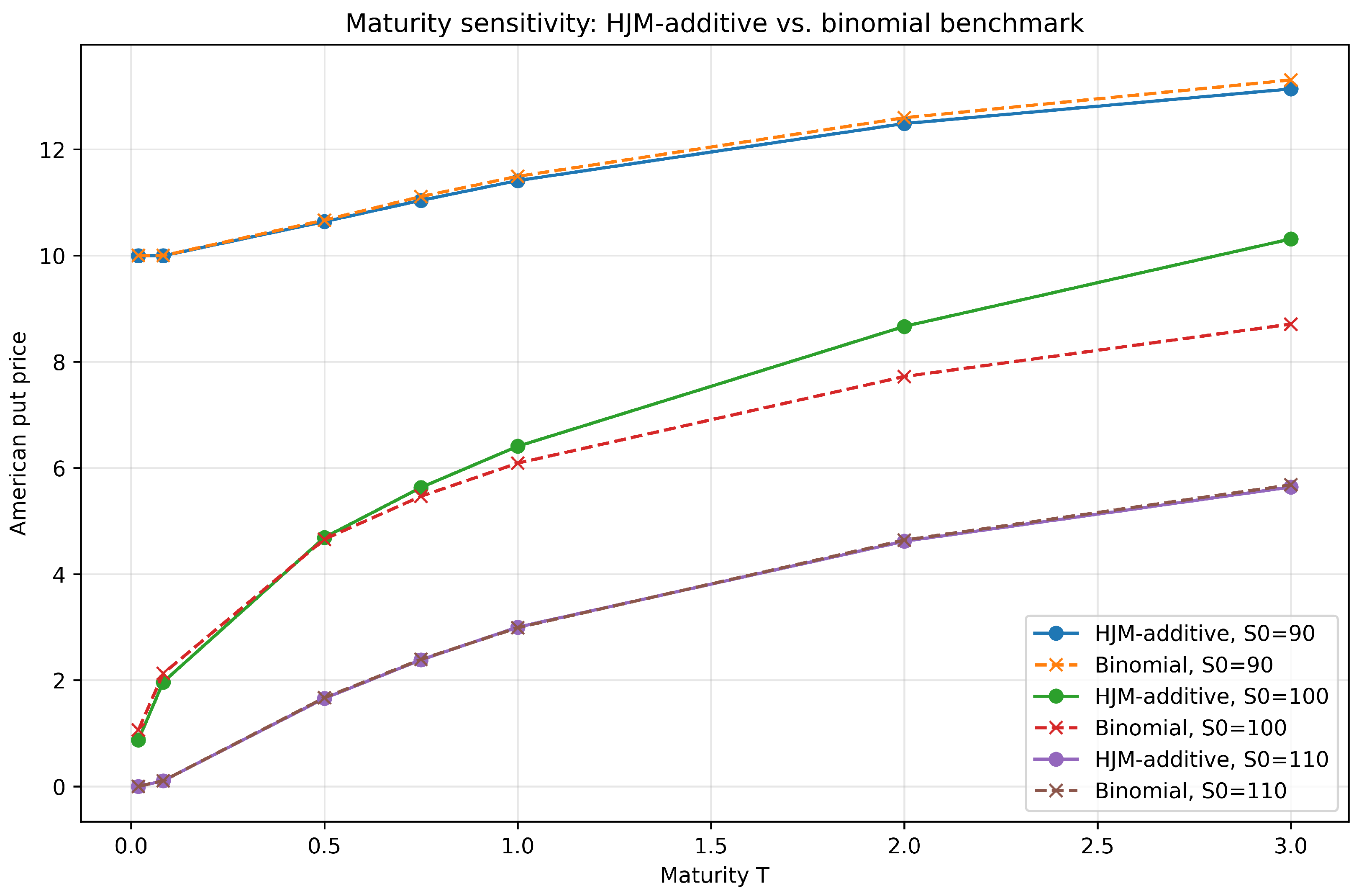
To address the sensitivity of the additive representation with respect to maturity, we isolate a maturity-only experiment from the broader robustness study. In this experiment, the strike is fixed at $K=100$, the risk-free rate $r=0.05$, HJM additive model approximation parameter $ϵ=0.5$, the stock volatility is fixed at $b=0.20$ and the initial stock prices are chosen to represent in-the-money ($S_0=90$), at-the-money($S_0=100$), and out-of-the-money ($S_0=110$) cases. For each value of $S_0$, we vary maturity over $T\in \{1/52,1/12,6/12,9/12,1,2,3\}$. This design allows us to examine the effect of time to maturity while holding the remaining model inputs fixed. The HJM additive prices are compared against the CRR binomial benchmark.

Figure 2 shows that the additive representation remains close to the binomial benchmark for the in-the-money and out-of-the-money cases across the full maturity range. For $S_0=90$, the HJM additive method slightly underprices the benchmark, with the absolute error increasing gradually as maturity increases. For $S_0=110$, the pricing errors remain very small across all maturities. The largest deviations occur in the at-the-money case $S_0=100$, especially for longer maturities. In this case, the HJM additive price overestimates the binomial benchmark for medium and long maturities, with the discrepancy increasing as maturity grows. This behavior is consistent with the structure of the additive representation. Near the money, the payoff kink at $S=K$, the local time contribution in the Tanaka decomposition, and the early-exercise boundary play a more prominent role. Since the numerical implementation approximates the local time density using a Gaussian kernel, errors in this approximation can accumulate over longer maturities. Thus, the maturity experiment indicates that the additive representation is numerically stable away from the at-the-money region, while the at-the-money long-maturity case is the most sensitive configuration.

4.1.5. Example 5

To investigate the source of the relatively large pricing error ($0.2851$) observed near the at-the-money case, in Example 1, we conduct a targeted numerical experiment focused on the American put with $S_0=100$, $K=100$, $r=0.05$, $b=0.20$, and $T=1$. The underlying stock price is simulated under the risk-neutral geometric Brownian motion using 200 time steps and 50,000 Monte Carlo paths in each replication. For each simulated sample, we first compute the American put value and the associated pathwise stopping rule using the LSMC method with the polynomial basis $[1,S,S^2]$ applied only to in-the-money paths. We then compare this with a CRR binomial tree benchmark computed with 1000 steps.

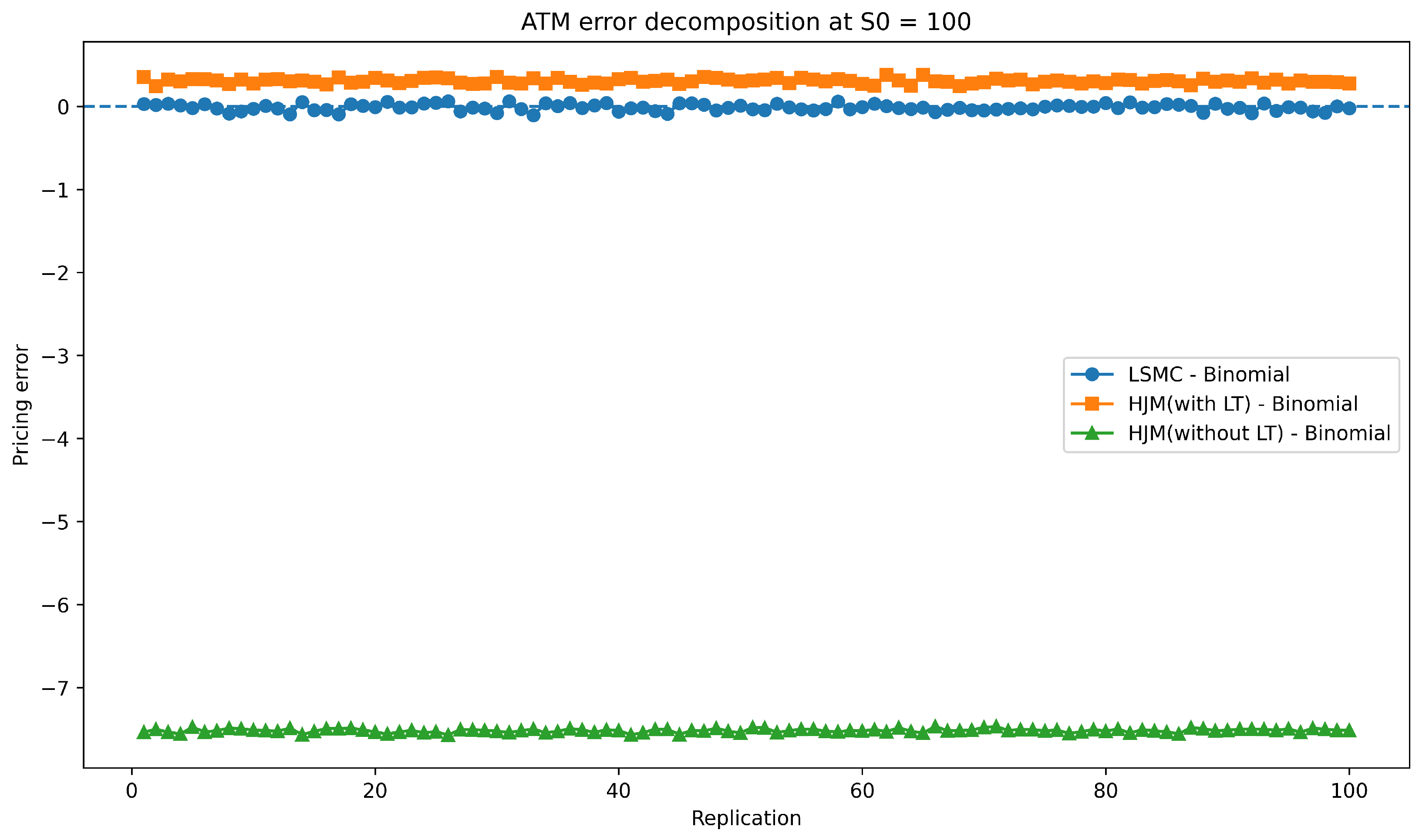
The main objective of this experiment is to decompose the additive model error into several interpretable components. To that end, for each replication, we compute five quantities: the binomial benchmark price, the LSMC price, the price induced directly by the LSMC stopping rule, the additive HJM price with the local time term included, and the additive HJM price with the local time term omitted. In the additive valuation, the local time contribution is approximated by a Gaussian kernel estimator with bandwidth $\epsilon =0.50$. Repeating this procedure over 100 independent replications allows us to assess whether the discrepancy near $S_0=100$ is driven primarily by the LSMC approximation of the stopping time, by the additive integration step conditional on the same stopping rule, or by the treatment of the local time term itself.

More specifically, the experiment reports the errors of the LSMC price and the stopping-rule-induced price relative to the binomial benchmark, the errors of the additive price with and without the local time term, the incremental contribution of the local time correction, and the residual additive integration error conditional on the same estimated stopping rule. In this way, the numerical setup provides a structured diagnostic of the at-the-money pricing error rather than only a single aggregate discrepancy measure.

The summary results are given in

Table A5. Mean errors and standard deviations from the at-the-money diagnostic experiment comparing LSMC, stopping-rule-induced, HJM-with-local-time, and HJM-without-local-time prices relative to the CRR binomial benchmark.

Metric Description	Value
Mean LSMC error vs. binomial	−0.0145
Std. dev. LSMC error vs. binomial	0.0397
Mean stopping rule price error vs. binomial	−0.0145
Std. dev. stopping rule price error vs. binomial	0.0397
Mean HJM with local time error vs. binomial	0.3036
Std. dev. HJM with local time error vs. binomial	0.0288
Mean HJM-without local time error vs. binomial	−7.5169
Std. dev. HJM without local time error vs. binomial	0.0226
Mean increment from local time	7.8206
Std. dev. increment from local time	0.0392
Mean additive integration error given same stopping rule	0.3182
Std. dev. additive integration error given same stopping rule	0.0511

, showing that the LSMC approximation is not the main source of the discrepancy: the mean LSMC error relative to the binomial benchmark is only $-0.0145$, indicating that the estimated stopping rule is accurate on average. By contrast, the local time term is crucial. When it is included, the mean HJM additive error is $0.3036$, which is close to the large discrepancy observed in Table 1 at $S_0=100$; when it is omitted, the mean error deteriorates dramatically to $-7.5169$. The mean incremental contribution of the local time term is $7.2056$, showing that neglecting this term produces a very large downward bias near the money. After including the local time correction, the remaining discrepancy is attributable mainly to the numerical approximation of the additive pricing formula itself, rather than to the stopping-rule estimation. Thus, the evidence indicates that the relatively large error at $S_0=100$ is driven primarily by the importance of the local time term and its numerical treatment, not by a failure of the LSMC stopping time approximation. Figure 3 illustrates this graphically.

4.2. European Put: Numerical Consistency with the Black-Scholes Benchmark

The theoretical results in Lemma 4 show that, when early exercise is absent, the proposed HJM additive representation is consistent with the classical risk-neutral valuation framework. To complement this theoretical result, we include a numerical experiment for a European put option. The purpose of this experiment is to verify, in a direct computational setting, that the HJM additive representation reproduces the standard Black-Scholes European put values when the optimal stopping feature is removed.

This experiment is useful for two reasons. First, it provides a benchmark case in which the correct option value is known in closed form. Second, it isolates the effect of the forward drift representation from the additional numerical complications introduced by early exercise. In the American case, the implementation depends on the estimated stopping rule and the approximation of the continuation region. In the European case, exercise occurs only at maturity, so the comparison with the Black-Scholes formula gives a more direct test of the valuation representation itself.

Example 6

We consider a European put option under the same risk-neutral stock price dynamics used in the previous numerical examples. The strike price, risk-free rate, volatility, and maturity are fixed at $K=100, r=0.05, b=0.20, T=1$. The initial stock price is varied over $S_0\in \{80,85,90,95,100,105,110,115,120\},$ so that the experiment covers in-the-money, at-the-money, and out-of-the-money cases. For each value of $S_0$, we compute three prices: the HJM additive value, CRR binomial, and the closed-form Black-Scholes European put price. The HJM additive value is computed using the same approach as in the previous American put experiments. However, because the option is European, there is no early-exercise decision, and no estimated stopping boundary is needed. The local time contribution arising from the payoff kink at the strike is approximated using the same Gaussian kernel method used in the American put examples with bandwidth parameter $ϵ=0.5$. This allows the European experiment to serve as a consistency check for the numerical implementation while keeping the computational framework aligned with the preceding American option experiments. The CRR binomial value was calculated using a 1000-step binomial tree. The results are reported in

Table 2. European put prices: HJM additive approximation ($ϵ=0.5$), CRR binomial estimate, and Black-Scholes benchmark with $K=100$, $r=0.05$, $b=0.20$, and $T=1$.

S0	HJM Additive	Binomial	Black Scholes	|HJM-BS|	|Bin-BS|
80	16.9758	16.9826	16.9824	0.0065	0.0002
85	13.3288	13.3360	13.3365	0.0077	0.0006
90	10.2171	10.2151	10.2142	0.0029	0.0009
95	7.6243	7.6325	7.6338	0.0095	0.0013
100	5.5733	5.5715	5.5735	0.0002	0.0020
105	3.9702	3.9807	3.9808	0.0106	0.0001
110	2.7936	2.7873	2.7859	0.0077	0.0015
115	1.9137	1.9125	1.9135	0.0002	0.0010
120	1.2933	1.2928	1.2920	0.0013	0.0008

.

Table 2 shows that the HJM additive values are close to the Black-Scholes benchmark across the full range of initial stock prices. This agreement is observed for in-the-money, at-the-money, and out-of-the-money options. The standard CRR binomial estimates also track the Black-Scholes values closely, as expected. The small differences between the HJM additive values and the Black-Scholes benchmark are due to numerical approximation error. In particular, the HJM additive implementation uses a Monte Carlo simulation, time discretization of the valuation integral, and a Gaussian kernel approximation of the local time term. These sources of error are absent from the closed-form Black-Scholes formula. Nevertheless, the numerical results confirm that the HJM additive representation reproduces the classical European valuation framework to a high degree of accuracy. This experiment therefore provides a useful numerical validation of the theoretical consistency result. In the absence of early exercise, the proposed additive representation does not introduce a different valuation principle; rather, it recovers the standard Black-Scholes European put prices up to numerical approximation error. The European case consequently serves as a benchmark confirming that the proposed framework is consistent with classical option pricing before the additional complexity of American-style exercise is introduced.

4.3. Modeling a Term Structure of European Put Prices Across Maturities

The multiplicative forward-rate framework is most naturally suited for modeling a term structure of option prices across maturities. In contrast to the additive representation, which is designed to incorporate the early-exercise premium of an American option, the multiplicative model should be interpreted as a dynamic model for the maturity-indexed price curve $T\mapsto V_t\left(T\right).$ Thus, the objective of this section is not to solve an optimal stopping problem. Rather, the goal is to illustrate how a given option price curve can be represented through multiplicative forward rates and how this curve evolves when those forward rates are assigned HJM-type stochastic dynamics. For a fixed observation time t, the multiplicative representation is

$$V_t\left(T\right)=V_t\left(t\right)exp\left(-{\int }_t^T{f}_t\left(u\right)du\right),$$

where $f_t\left(T\right)$ is the multiplicative forward rate associated with the option price curve. The quantity $f_t\left(T\right)$ is not an interest-rate forward rate. Instead, it measures the rate at which the logarithm of the option value changes with respect to maturity. Whenever the maturity map $T\mapsto V_t\left(T\right)$ is differentiable and strictly positive, we define $f_t\left(T\right)=-{\displaystyle \frac{\partial }{\partial T}}log{V}_t\left(T\right).$ This definition is directly analogous to extracting a forward-rate curve from a bond price curve in the classical HJM framework.

In the numerical examples below, we use European put options rather than American put options. This choice is intentional. Since European options do not involve an early-exercise decision, they provide a clean setting in which to illustrate the multiplicative term-structure representation. The multiplicative model is therefore being used here to describe and simulate the maturity curve of option prices, not to determine an optimal exercise boundary.

4.3.1. Example 7

We consider a European put option in the Black-Scholes setting with parameters $S_0=100, K=100, r=0.05, b=0.20$. The maturity grid is $T\in \{0.25,0.50,0.75,1.00,1.50,2.00\}$. For each maturity $T_j$, we first compute the Black-Scholes European put price $V^{BS}\left(T_j\right)$ using the closed form formula. These prices form the initial maturity-indexed option price curve. The next step is to convert this price curve into an initial multiplicative forward-rate curve. Since the maturity grid is discrete, we approximate $f_0\left(T\right)=-{\displaystyle \frac{\partial }{\partial T}}log{V}_0\left(T\right)$ by finite differences. For adjacent maturities $T_j$ and $T_{j+1}$, define $\Delta T_j=T_{j+1}-T_j.$ Then time-zero forward rate over the $j^{th}$ maturity interval is approximated by $f_0^{\left(j\right)}=-{\displaystyle \frac{log{V}^{BS}\left(T_{j+1}\right)-log{V}^{BS}\left(T_j\right)}{\Delta T_j}}.$ Thus, the forward rates are interval-based quantities. In this example, there are six maturities but only five maturity intervals, and hence five discrete forward rates.

After obtaining the forward rates, we reconstruct the original option price curve deterministically. Since the maturity grid begins at $T_1=0.25$, the reconstruction is anchored at $V^{BS}\left(T_1\right)$, rather than at $V^{BS}\left(0\right)$. This is important because, for an at-the-money put with $S_0=K$, the instantaneous maturity payoff is ${(K-S_0)}^{+}=0,$ and the logarithm of this value is not defined. Therefore, the numerical implementation uses the first strictly positive maturity price as the anchor. For $j\ge 2$, the reconstructed price is

$$V^{rec}\left(T_j\right)=V^{BS}\left(T_1\right)exp\left(-{\displaystyle \sum _{i=1}^{j-1}}{f}_0^{\left(i\right)}\Delta T_i\right).$$

Equivalently, this is the discrete version of

$$V^{rec}\left(T\right)=V^{BS}\left(T_1\right)exp\left(-{\int }_{T_1}^T{f}_0\left(u\right)du\right).$$

Because the initial forward rates are computed directly from the Black-Scholes price curve, the deterministic reconstruction simply reverses the logarithmic finite-difference calculation. Hence, the reconstructed curve matches the original Black-Scholes curve up to numerical precision. This confirms that the multiplicative representation can encode the initial maturity curve $T\mapsto V_0\left(T\right)$ in forward-rate form.

However, this reconstruction is only a static verification: it represents the option price curve at the initial time and does not describe how the curve evolves. To illustrate the dynamic role of the multiplicative HJM framework, we next allow the forward-rate curve to evolve stochastically. This step shows how the entire maturity-indexed option price curve $T\mapsto V_t\left(T\right)$ may move over time in an arbitrage-consistent way. The next step is therefore to illustrate the stochastic HJM evolution of this forward-rate curve. We assume a one-factor multiplicative HJM specification given in Equation (34). For simplicity, we use a constant forward-rate volatility ${\beta }_t\left(T\right)=\beta ,$ with $\beta =0.3$. Under the multiplicative HJM no-arbitrage restriction, the drift is given by Equation (36). In the constant-volatility case, Equation (41) shows that this restriction on drift simplifies to ${\alpha }_t\left(T\right)={\beta }^2(T-t).$ In the discrete maturity-grid implementation, this drift is approximated over the maturity intervals used in the simulation.

Starting from the initial forward-rate curve extracted from the Black-Scholes prices, we simulate the forward rates using the Euler discretization

$$f_{t+\Delta t}^{\left(j\right)}=f_t^{\left(j\right)}+{\alpha }_t^{\left(j\right)}\Delta t+\beta \Delta W_t,\Delta W_t=\sqrt{\Delta t}{Z}_t,Z_t\sim N(0,1).$$

Here $f_t^{\left(j\right)}$ denotes the simulated multiplicative forward rate at time t on the maturity interval $[T_j,T_{j+1}]$, and ${\alpha }_t^{\left(j\right)}$ denotes the corresponding drift for that interval. In the simulation, we use $\Delta t=0.01$ over 200 time steps. The same Brownian increment is applied to all maturity intervals, so this is a one-factor simulation of the entire forward-rate curve. At the end of the simulation, the terminal forward-rate curve is converted back into an option price curve using the same multiplicative reconstruction formula:

$$V^{sim}\left(T_j\right)=V^{BS}\left(T_1\right)exp\left(-{\displaystyle \sum _{i=1}^{j-1}}{f}_{sim}^{\left(i\right)}\Delta T_i\right).$$

This produces one simulated future maturity curve of European put prices.

Table 3. Black–Scholes European put prices, multiplicative forward-rate reconstruction, and simulated multiplicative HJM prices across maturities, with $S_0=K=100$, $r=0.05$, $b=0.20$, and forward-rate volatility $\beta =0.30$.

T	BS Price	Reconstructed	Simulated	|Rec-BS|	|Sim-BS|
0.25	3.3728	3.3728	3.3728	0.0000	0.0000
0.50	4.4197	4.4197	3.6648	0.0000	0.7549
0.75	5.0917	5.0917	3.4619	0.0000	1.6298
1.00	5.5735	5.5735	3.0727	0.0000	2.5008
1.50	6.2173	6.2173	2.1548	0.0000	4.0624
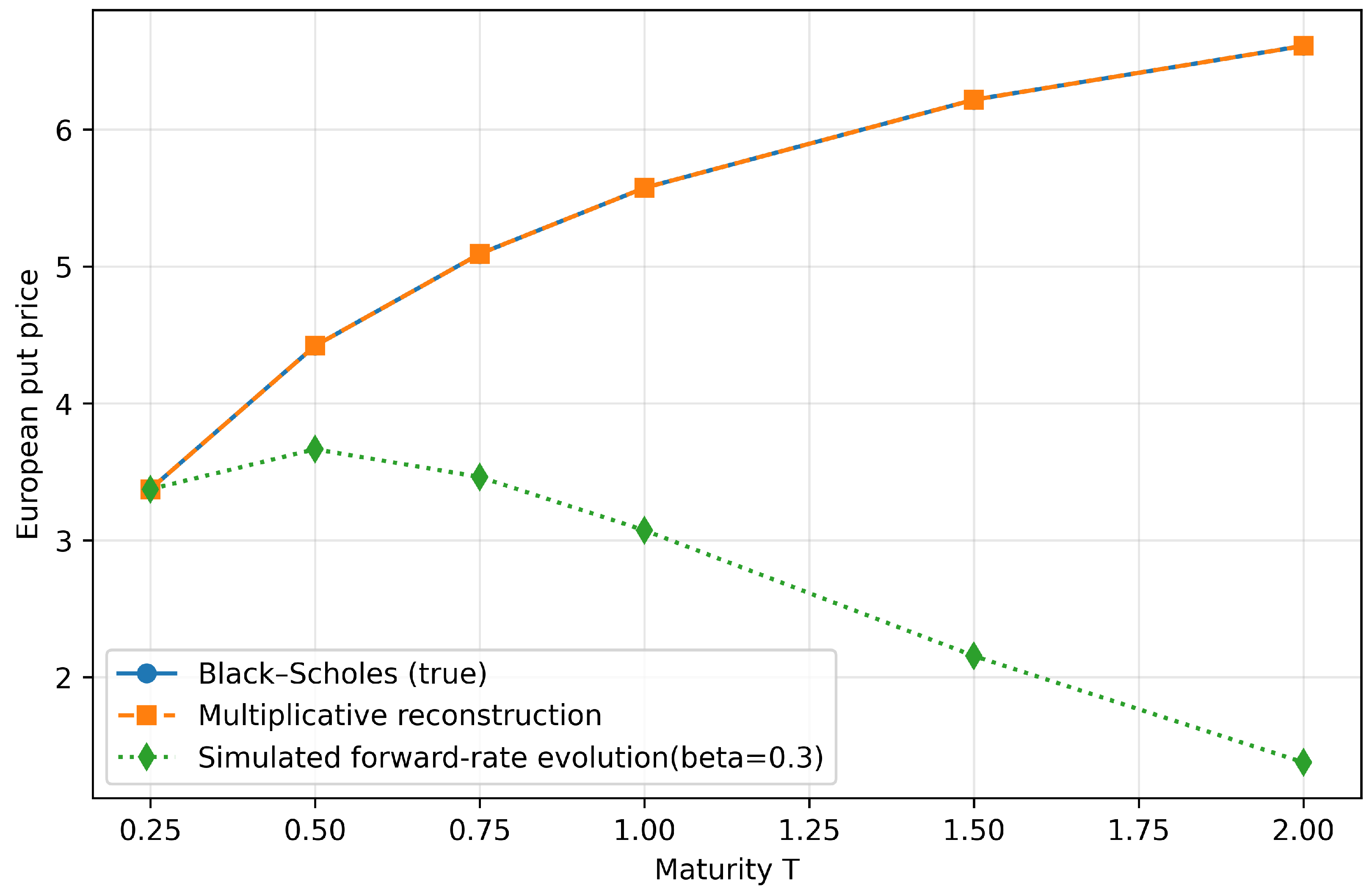
2.00	6.6105	6.6105	1.3773	0.0000	5.2332

and Figure 4 compare three objects:

• the Black-Scholes benchmark curve $V^{BS}\left(T\right)$;
• the deterministic multiplicative reconstruction $V^{rec}\left(T\right)$;
• the HJM multiplicative model based simulated curve $V^{sim}\left(T\right)$ obtained after stochastic evolution of the forward rates.

The reconstructed prices agree with the Black-Scholes prices up to numerical precision. This confirms that the multiplicative representation is internally consistent: if the forward rates are extracted from a given price curve, integrating those same forward rates reconstructs the original curve. By contrast, the HJM-simulated curve is not expected to coincide with the Black-Scholes curve path by path. Once a nonzero forward-rate volatility $\beta$ is introduced, the forward-rate curve evolves randomly. Therefore, the simulated price curve represents one possible stochastic evolution of the initial maturity structure, rather than a deterministic reproduction of the original Black-Scholes prices. In this sense, the purpose of the simulation is not to improve upon the Black-Scholes formula for a single European option. Instead, it demonstrates how the multiplicative HJM model can be used to generate dynamic, arbitrage-consistent movements of an entire option price term structure.

The results show two distinct effects. First, the deterministic reconstruction matches the Black-Scholes curve exactly, confirming that the multiplicative representation correctly encodes the initial maturity curve. Second, the simulated curve differs from the Black-Scholes benchmark because the forward rates have been allowed to evolve stochastically with $\beta =0.3$. The discrepancy increases with maturity because longer maturities accumulate more forward-rate variation through the integral ${\int }_{T_1}^T{f}_t\left(u\right)du.$ Thus, the example illustrates both the exact encoding of an initial option price curve and the stochastic evolution of that curve under the multiplicative HJM dynamics.

4.3.2. Example 8

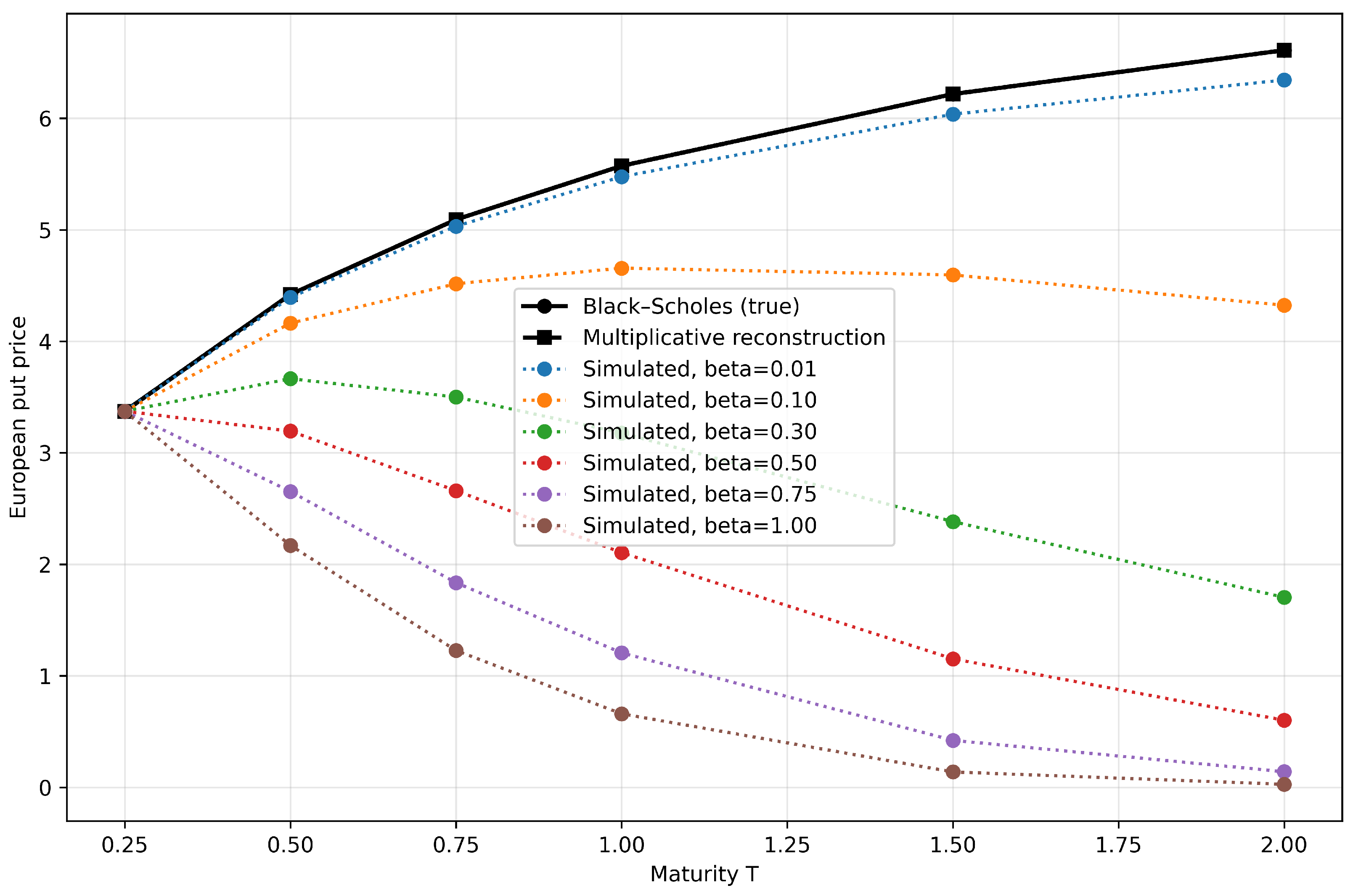
To examine the effect of the forward volatility parameter in the multiplicative model, we conduct a sensitivity experiment in which the constant parameter $\beta$ is varied over a grid from $0.01$ to $1.00$. The purpose of this experiment is to show how the size of $\beta$ affects the simulated maturity curve generated by the HJM dynamics. The initial European put term structure is first generated under the Black-Scholes model with the parameters $S_0=100$, $K=100$, $r=0.05$, and $b=0.20$ on the maturity grid $T\in \{0.25,0.5,0.75,1.0,1.5,2.0\}$. From these prices, we compute the initial multiplicative forward rate curve using the discrete approximation $f_0\left(T\right)\approx -{\partial }_{T}ln{V}_0\left(T\right)$. For each value of $\beta$, we then simulate a one-factor HJM-type evolution of the forward rates over 200 time steps, using Equation (34), with step size $dt=0.01$, starting from the same initial forward curve. The simulated terminal forward rate curve is subsequently transformed back into an option-price term structure using the multiplicative reconstruction formula. This setup allows us to compare, across different values of $\beta$, the resulting forward rate curves, the simulated option-price term structures, and their deviations from the original Black-Scholes benchmark. A detailed price comparison for selected beta values is given in

Table A6. Detailed beta-sensitivity results for the multiplicative HJM simulation, comparing Black–Scholes European put prices with simulated prices across selected forward-rate volatility values $\beta$ and maturities.

$\mathit{\beta }$	T	BS Price	Simulated Price	|BS-Sim|
0.01	0.25	3.3728	3.3728	0.0000
0.01	0.50	4.4197	4.3938	0.0259
0.01	0.75	5.0917	5.0322	0.0596
0.01	1.00	5.5735	5.4760	0.0975
0.01	1.50	6.2173	6.0369	0.1804
0.01	2.00	6.6105	6.3435	0.2670
0.10	0.25	3.3728	3.3728	0.0000
0.10	0.50	4.4197	4.1626	0.2572
0.10	0.75	5.0917	4.5164	0.5753
0.10	1.00	5.5735	4.6562	0.9174
0.10	1.50	6.2173	4.5957	1.6216
0.10	2.00	6.6105	4.3235	2.2870
0.30	0.25	3.3728	3.3728	0.0000
0.30	0.50	4.4197	3.6648	0.7549
0.30	0.75	5.0917	3.5009	1.5908
0.30	1.00	5.5735	3.1776	2.3959
0.30	1.50	6.2173	2.3832	3.8340
0.30	2.00	6.6105	1.7037	4.9068
0.50	0.25	3.3728	3.3728	0.0000
0.50	0.50	4.4197	3.1946	1.2251
0.50	0.75	5.0917	2.6602	2.4315
0.50	1.00	5.5735	2.1048	3.4687
0.50	1.50	6.2173	1.1527	5.0645
0.50	2.00	6.6105	0.6017	6.0088
0.75	0.25	3.3728	3.3728	0.0000
0.75	0.50	4.4197	2.6534	1.7663
0.75	0.75	5.0917	1.8352	3.2565
0.75	1.00	5.5735	1.2061	4.3675
0.75	1.50	6.2173	0.4216	5.7957
0.75	2.00	6.6105	0.1405	6.4700
1.00	0.25	3.3728	3.3728	0.0000
1.00	0.50	4.4197	2.1699	2.2498
1.00	0.75	5.0917	1.2273	3.8644
1.00	1.00	5.5735	0.6596	4.9139
1.00	1.50	6.2173	0.1383	6.0790
1.00	2.00	6.6105	0.0276	6.5829

.

Figure 5 illustrates the sensitivity of the multiplicative model to the forward volatility parameter $\beta$. As expected, the multiplicative reconstruction coincides almost exactly with the Black-Scholes term structure, confirming that the representation is internally consistent when applied to a deterministic initial curve. By contrast, the simulated price curves deviate increasingly from the Black-Scholes benchmark as $\beta$ rises. For very small values, such as $\beta =0.01$, the simulated curve remains close to the original term structure across all maturities. However, as $\beta$ increases, the simulated curves bend downward and progressively understate long-maturity put prices. This effect becomes substantial for $\beta \ge 0.30$ and is especially pronounced at $T=1.5$ and $T=2.0$. The figure therefore shows that the forward volatility parameter has a cumulative impact on the reconstructed option-price curve, with larger values of $\beta$ generating stronger departures from the initial market-consistent term structure. This sensitivity highlights the importance of calibrating $\beta$ to market data rather than selecting it arbitrarily.

A natural question is why the HJM-simulated curves lie below the initial European put price term structure. This occurs because, when the forward-rate volatility $\beta$ is nonzero, the multiplicative HJM drift restriction introduces a positive drift in the forward-rate process. As the simulated forward rates increase, the cumulative integral ${\int }_{T_1}^T{f}_t\left(u\right)du$ becomes larger, which reduces the reconstructed price $V_t\left(T\right)=V_t\left(T_1\right)exp\left(-{\int }_{T_1}^T{f}_t\left(u\right)du\right).$ The effect becomes stronger for longer maturities because the integral is accumulated over a larger interval. Thus, the simulated price matches the Black-Scholes price at the initial maturity due to initialization, but the gap widens as maturity increases, as shown in Figure 5.

5. Calibration to Market Data

The preceding sections developed the additive and multiplicative forward drift representations as theoretical valuation frameworks and illustrated them with numerical experiments under Black-Scholes dynamics. A natural and important question, raised in the refereeing process, is how the forward drift processes $\left\{f_t\left(T\right)\right\}$ could be calibrated to real market data. In this section, we outline calibration strategies for both models, discuss the data requirements and computational considerations involved, and identify the main challenges that arise in practice.

5.1. Calibration of the Multiplicative Model

The multiplicative model is more straightforward to calibrate than the additive model because its forward rate is defined directly from the observed maturity curve of option values. In practice, however, calibration is performed not on raw market quotes themselves, but on a smoothed and arbitrage-consistent fitted term structure obtained from those quotes.

5.1.1. Extracting the Initial Forward Rate Curve

Fix an observation time t, and suppose that option prices ${\left\{V_t^{\mathrm{mkt}}\left(T_j\right)\right\}}_{j=1}^J$ are observed for a common strike across maturities $T_1<T_2<\cdots <T_J$. After interpolation and smoothing, let ${\tilde{V}}_t\left(T\right)$ denote the fitted maturity-price curve. The initial forward rate is then defined by

$$f_t\left(T\right)=-{\displaystyle \frac{\partial }{\partial T}}ln{\tilde{V}}_t\left(T\right).$$

(47)

When the data are available only on a discrete maturity grid, a finite-difference approximation may be used:

$${\widehat{f}}_t\left(T_j\right)\approx -{\displaystyle \frac{ln{\tilde{V}}_t\left(T_{j+1}\right)-ln{\tilde{V}}_t\left(T_j\right)}{T_{j+1}-T_j}},j=1,\dots ,J-1.$$

(48)

Because differentiation amplifies noise, the smoothing stage is essential. A practical calibration pipeline proceeds as follows:

• Quote cleaning. Filter illiquid or unreliable observations using bid-ask spreads, volume, and open interest.
• Curve fitting. Fit a smooth maturity-price curve $T\mapsto {\tilde{V}}_t\left(T\right)$ to the filtered quotes. In practice, one may fit either option prices directly or a transformed object such as implied volatility, provided the resulting fitted curve is sufficiently smooth for differentiation.
• Forward rate extraction. Compute the initial forward curve from Equation (47), either analytically from the fitted parametrization or numerically on a refined maturity grid.

Once $f_t\left(T\right)$ has been extracted from the fitted curve, the multiplicative representation ${\tilde{V}}_t\left(T\right)={\tilde{V}}_t\left(t\right)exp\left(-{\int }_t^T{f}_t\left(u\right)du\right)$ reproduces the fitted maturity curve by construction. Thus, the initial cross sectional calibration is exact relative to the smoothed term structure, though not necessarily relative to every raw market quote.

5.1.2. Calibrating the Forward Rate Dynamics

The initial forward curve describes the cross section at time t, but dynamic simulation requires a specification of the forward rate volatility ${\beta }_t\left(T\right)$ in Equation (34) with drift ${\alpha }_t\left(T\right)$ determined by the no-arbitrage restriction given in Equation (36). In the one-factor constant-volatility case, ${\beta }_t\left(T\right)\equiv \beta$, and the drift takes the corresponding simplified form given by Equation (41). More generally, ${\beta }_t\left(T\right)$ may be modeled as a function of time to maturity. In practice, the volatility term may be estimated in several ways.

• Historical estimation. If a time series of option-price curves is available, one may first construct a sequence of fitted forward curves $\left\{f_{t_i}\left(T\right)\right\}$, and then estimate the volatility of forward rate innovations. For a fixed time to maturity $\tau =T-t$, define

  $$\Delta f_{t_i}\left(\tau \right):=f_{t_{i+1}}(t_{i+1}+\tau )-f_{t_i}(t_i+\tau ).$$

  (49)
  The sample variability of these increments yields an empirical estimate of $\beta \left(\tau \right)$. Since these increments are themselves computed from smoothed option data, the resulting estimate should be viewed as a market-informed proxy rather than a noise-free observation of the true forward rate volatility.
• Parametric volatility specification. A tractable alternative is to posit a parametric form such as a constant volatility ${\beta }_t\left(T\right)=\beta$, an exponentially decaying specification ${\beta }_t\left(T\right)={\beta }_0{e}^{-\kappa (T-t)}$, or a piecewise constant function over maturity buckets. The parameters may then be estimated either from historical forward rate innovations or by fitting model-implied dynamics to the option panel data.
• Panel-data calibration. Given the option prices observed across multiple dates and maturities, one may estimate the parameters $\theta$ of a chosen volatility specification by minimizing

  $$\underset{\theta }{min}\sum _{i,j}{w}_{ij}{\left(V_{t_i}^{\mathrm{model}}(T_j;\theta )-V_{t_i}^{\mathrm{mkt}}\left(T_j\right)\right)}^2,$$

  (50)

  where the weights $w_{ij}$ may be selected to reflect liquidity or vega sensitivity.

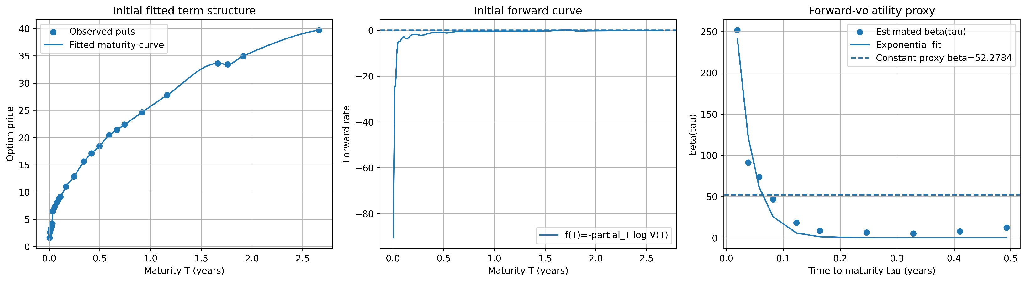
In the empirical illustration of this paper, we adopt the simplest market-informed version of this program. We first fit an initial maturity-price curve from observed option quotes and extract the corresponding initial forward curve. We then estimate a constant volatility parameter $\beta$ from recent changes in the fitted forward curve across maturities. The resulting simulation should be interpreted as a market-informed illustration of the multiplicative model rather than as a full institutional-grade calibration engine.

5.1.3. Example 9

The calibration exercise in this section is intended as a simplified market-informed illustration of the multiplicative model rather than a full empirical calibration study. The procedure consists of four steps. First, we obtain a contemporaneous cross section of listed AAPL put-option quotes from Yahoo Finance through yfinance. The data are filtered to retain only contracts with positive mid prices, open interest of at least 10, and relative bid-ask spreads not exceeding 35%. Second, we restrict attention to a single strike that is common across the selected expirations and closest to the observed spot price. This produces a maturity-indexed panel of put prices for one fixed strike. Third, we fit a smooth initial maturity-price curve to the filtered option prices using a shape-preserving interpolation method. This fitted curve is used to extract the initial multiplicative forward curve. Fourth, we estimate a constant forward volatility parameter from recent changes in the fitted forward curve across maturities. The calibrated parameter is therefore the constant forward volatility proxy in the simplified multiplicative specification, while the initial forward curve is obtained directly from the fitted market price curve.

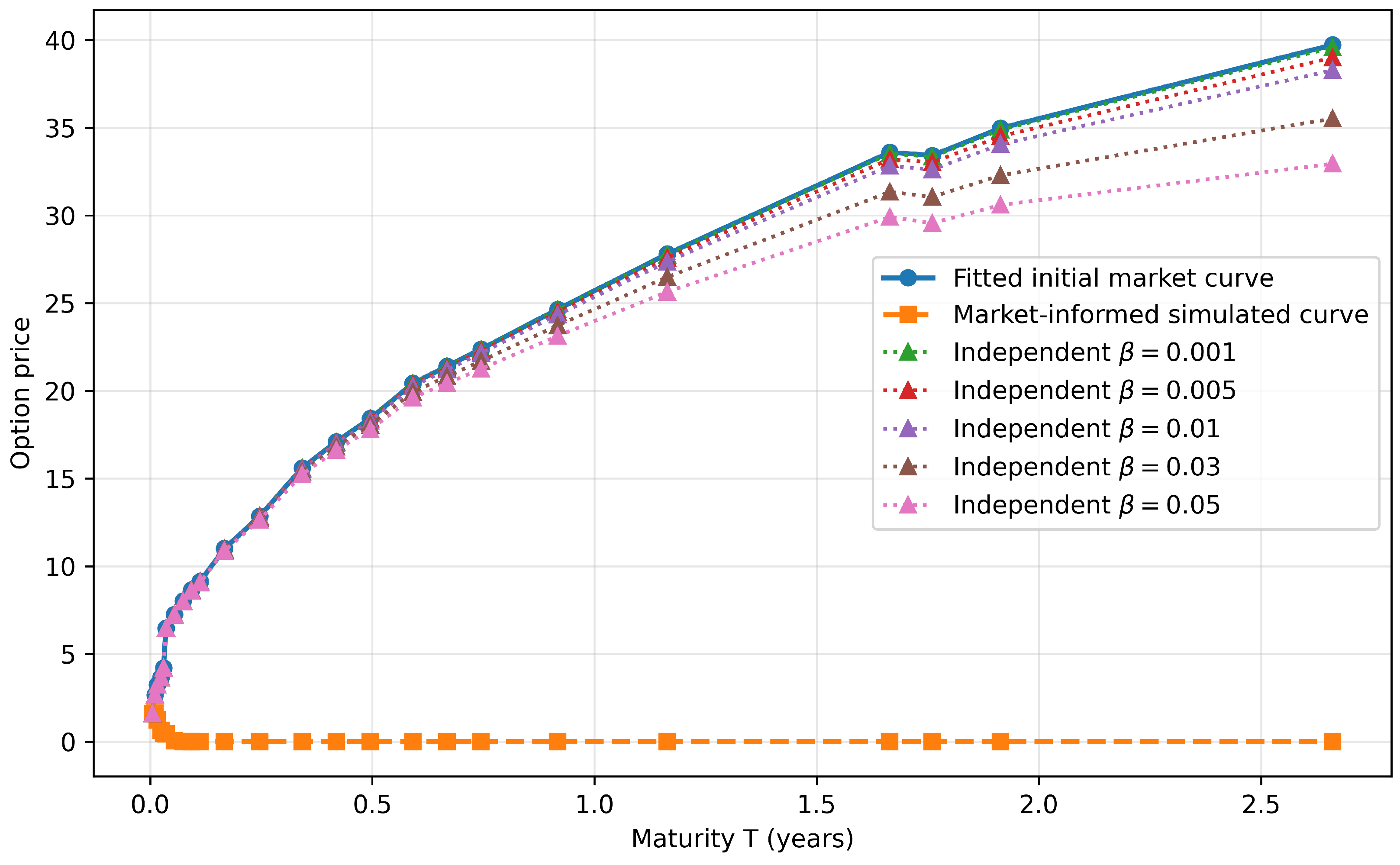
The quality of the calibration is assessed in two ways. The fit of the initial maturity-price curve is checked by comparing the fitted prices with the observed market mid prices at the selected maturities. The adequacy of the simplified dynamic specification is then assessed by comparing the fitted initial market curve with the simulated curve generated by the multiplicative model using the estimated volatility proxy. Because the example uses a single constant volatility parameter, the simulated curve is not expected to reproduce all features of the observed market term structure. Thus, the calibration results should be interpreted as evidence of the feasibility and limitations of the proposed workflow, rather than as a production-level calibration to option market data.

For the market-informed numerical illustration of the multiplicative model, we use put-option data for the ticker AAPL, obtained through yfinance from Yahoo Finance. On the script execution date, 18 April 2026, we collected the contemporaneous cross section of listed AAPL put options and selected a single strike, $K=270.00$, which is common across expirations and closest to the observed spot price $S_0=270.23$. Since these are single-name U.S. equity options, the quoted contracts are American-style by market convention. Accordingly, this example should be interpreted as a market-informed illustration of the multiplicative calibration workflow applied to an observed put-price term structure, rather than as a strict calibration to a purely European option market. To improve quote quality, we retain only contracts with strictly positive mid prices, open interest of at least 10, and relative bid-ask spreads not exceeding $35\%$, where the relative spread is defined as $(\mathrm{ask}-\mathrm{bid})/\mathrm{mid}$ and $\mathrm{mid}=(\mathrm{bid}+\mathrm{ask})/2$. The expiration dates of the selected AAPL put contracts determine the maturity grid, with time to maturity measured in year fractions from the observation date to each expiration date. We then fit a smooth maturity-price curve, $T\mapsto {\tilde{V}}_t\left(T\right)$, by interpolating the filtered market prices with a shape-preserving spline; this fitted curve serves as the continuous term structure from which the multiplicative forward curve is extracted via $f_t\left(T\right)=-{\partial }_{T}ln{\tilde{V}}_t\left(T\right)$. To obtain a market-informed proxy for the forward volatility term, we use daily historical data for the same selected option contracts over the preceding one-month window, specified in the code by HISTORY_PERIOD = “1mo”. These daily observations are converted into fitted forward curves on maturity buckets corresponding to $\tau \in \{7,14,21,30,45,60,90,120,150,180\}$ calendar days. For each fixed time to maturity $\tau$, we then compute the forward rate innovations $\Delta f_{t_i}\left(\tau \right)$ using the historical estimation approach described earlier, and use the sample variability of these increments as a market-informed proxy for the forward volatility function $\beta \left(\tau \right)$. Thus, $\beta \left(\tau \right)$ is inferred from the empirical day-to-day fluctuations of the fitted forward curve. For simplicity, we also report a constant-$\beta$ proxy obtained by averaging the estimated values across maturity buckets. This estimated constant volatility parameter is then used in Equations (34) and (41) to generate a one-factor illustrative simulation of the multiplicative model, and the resulting simulated maturity-price curve is compared with the initial fitted AAPL put term structure.

Table A7. Market observations for AAPL put options.

Expiration	T	Strike	Bid	Ask	Last	Mid	OI	Vol
2026-04-20	0.0055	270.0	1.56	1.65	1.60	1.60	67	16,249
2026-04-22	0.0110	270.0	2.56	2.75	2.65	2.66	31	1593
2026-04-24	0.0164	270.0	3.15	3.35	3.26	3.25	2702	4727
2026-04-27	0.0246	270.0	3.45	3.85	3.70	3.65	81	219
2026-04-29	0.0301	270.0	4.05	4.35	4.15	4.20	19	267
2026-05-01	0.0356	270.0	6.35	6.60	6.35	6.48	259	1094
2026-05-08	0.0548	270.0	7.10	7.40	7.30	7.25	72	230
2026-05-15	0.0739	270.0	7.95	8.10	8.02	8.02	14,970	1862
2026-05-22	0.0931	270.0	8.45	8.85	8.55	8.65	233	51
2026-05-29	0.1123	270.0	8.95	9.30	9.25	9.12	24	375
2026-06-18	0.1670	270.0	10.90	11.10	10.97	11.00	3734	1103
2026-07-17	0.2464	270.0	12.75	12.95	12.90	12.85	1561	254
2026-08-21	0.3422	270.0	15.50	15.70	15.60	15.60	1945	920
2026-09-18	0.4189	270.0	17.00	17.20	17.00	17.10	4758	177
2026-10-16	0.4956	270.0	18.35	18.50	18.40	18.42	367	3273
2026-11-20	0.5914	270.0	20.20	20.65	20.20	20.42	108	5
2026-12-18	0.6680	270.0	21.30	21.50	21.40	21.40	3007	233
2027-01-15	0.7447	270.0	22.25	22.50	22.39	22.38	6304	84
2027-03-19	0.9172	270.0	24.35	24.95	24.90	24.65	321	90
2027-06-17	1.1636	270.0	27.65	27.95	27.83	27.80	1961	69
2027-12-17	1.6646	270.0	32.15	35.05	32.15	33.60	562	2
2028-01-21	1.7604	270.0	32.75	34.10	33.93	33.42	584	6
2028-03-17	1.9138	270.0	34.20	35.75	38.15	34.98	289	11
2028-12-15	2.6612	270.0	39.05	40.40	39.63	39.72	210	39

presents real-world market data for AAPL put options used in the empirical validation of the pricing models. It includes strikes, time to maturity (T), and market prices derived from bid-ask midpoints.

Table A8. Observed AAPL put market prices and PCHIP-interpolated fitted prices evaluated at the observed maturities.

${\mathit{T}}_{\mathit{i}}$ (Years)	Observed Price ${\mathit{V}}_{\mathit{i}}\left({\mathit{T}}_{\mathit{i}}\right)$	Fitted Price ${\mathit{V}}_{\mathbf{fit}}\left({\mathit{T}}_{\mathit{i}}\right)$	Absolute Difference
0.0055	1.6050	1.6050	0.000000
0.0110	2.6550	2.6550	0.000000
0.0164	3.2500	3.2500	0.000000
0.0246	3.6500	3.6500	0.000000
0.0301	4.2000	4.2000	0.000000
0.0356	6.4750	6.4750	0.000000
0.0548	7.2500	7.2500	0.000000
0.0739	8.0250	8.0250	0.000000
0.0931	8.6500	8.6500	0.000000
0.1123	9.1250	9.1250	0.000000
0.1670	11.0000	11.0000	0.000000
0.2464	12.8500	12.8500	0.000000
0.3422	15.6000	15.6000	0.000000
0.4189	17.1000	17.1000	0.000000
0.4956	18.4250	18.4250	0.000000
0.5914	20.4250	20.4250	0.000000
0.6680	21.4000	21.4000	0.000000
0.7447	22.3750	22.3750	0.000000
0.9172	24.6500	24.6500	0.000000
1.1636	27.8000	27.8000	0.000000
1.6646	33.6000	33.6000	0.000000
1.7604	33.4250	33.4250	0.000000
1.9138	34.9750	34.9750	0.000000
2.6612	39.7250	39.7250	0.000000

presents the results of the curve-fitting process, comparing the observed AAPL market prices with the prices generated by the fitted curve across maturities T. As noted earlier, the fitted curve is obtained by interpolating the filtered market prices with a shape-preserving spline; accordingly, the fit is exact at the observed maturity points. Finally,

Table A9. Market-informed estimates of the multiplicative HJM forward-rate volatility $\widehat{\beta }\left(\tau \right)$ and the corresponding fitted exponential volatility curve ${\beta }_{\mathrm{fit}}\left(\tau \right)$ across maturity buckets.

$\mathit{\tau }$ (Maturity Buckets)	$\widehat{\mathit{\beta }}\left(\mathit{\tau }\right)$ (Market)	${\mathit{\beta }}_{\mathbf{fit}}$ (Model)
0.0192	251.9501	242.1000
0.0383	91.3633	122.1422
0.0575	73.7594	61.6221
0.0821	46.8018	25.5690
0.1232	18.3660	5.9021
0.1643	8.5722	1.3624
0.2464	6.5194	0.0726
0.3285	5.3100	0.0039
0.4107	7.7815	0.0002
0.4928	12.3600	0.0000

reports the estimated values of $\beta \left(\tau \right)$, computed from daily historical data, together with the corresponding fitted values obtained from the exponential specification applied to the $\beta \left(\tau \right)$ estimates.

Figure 6 reports the market-informed calibration results for the multiplicative model using the filtered AAPL put-option cross section. The left panel shows that the fitted maturity-price curve closely tracks the observed market quotes, indicating that the spline-based preprocessing provides a smooth and numerically stable term structure for forward rate extraction. The middle panel shows the corresponding initial forward curve, $f_t\left(T\right)=-{\partial }_{T}ln{\tilde{V}}_t\left(T\right)$, which is sharply negative at the very short end and then quickly flattens toward values near zero as maturity increases. This behavior reflects the steep slope of the fitted option-price curve close to expiration. The right panel reports the empirical proxy for the forward volatility function $\beta \left(\tau \right)$, which is very large for short maturities and decays rapidly as $\tau$ increases. When these estimated values are averaged to form a constant-$\beta$ proxy, the resulting value is dominated by the short-end observations. Consequently, the one-factor simulation using this constant volatility generates a maturity-price curve, given in Figure 7, that collapses toward zero and lies far below the fitted initial term structure. These results suggest that, in this dataset, a constant-$\beta$ specification is too crude to represent the highly maturity-dependent forward rate variability implied by market data. Thus, while the initial cross sectional fit is satisfactory, the simulation results indicate that a more flexible volatility specification, such as a maturity-dependent $\beta \left(\tau \right)$, is needed for a realistic dynamic implementation of the multiplicative model.

5.2. Calibration of the Additive Model

A full market calibration of the additive model is considerably more difficult than in the multiplicative case because the additive forward drift is not determined solely by the observed maturity-price curve. In the additive framework, the forward drift depends on the continuation region and hence on the optimal stopping rule, while the optimal stopping rule itself depends on the value function generated by that same forward drift. This creates a circular calibration problem. Although one may extract a market-informed proxy for the initial forward drift from the observed early-exercise premium, a full calibration would additionally require estimation of the exercise boundary and repeated updating of the value function until consistency is achieved. In practice, this is further complicated by the sparse maturity grid of listed American options, the need for interpolation and smoothing, and the additional numerical error introduced by estimating the stopping boundary. For these reasons, a full market calibration of the additive model would require a substantially more elaborate iterative procedure and would still rely on approximation at several stages. Accordingly, in the present paper, we do not pursue a full market calibration of the additive model and instead focus on its theoretical structure and controlled numerical illustrations.

5.3. Summary

The multiplicative model can be calibrated in a relatively standard fashion: the initial forward rate curve is extracted from observed option prices via numerical differentiation, and the forward rate volatility is estimated from historical data or cross sectional fitting. The additive model requires additional care due to the dependence of the forward drift on the optimal stopping boundary, but can be calibrated either by direct extraction from the maturity structure of the early-exercise premium or through an iterative scheme that alternates between boundary estimation and forward drift computation. Both approaches are anchored by the spot consistency condition, which provides a model-free constraint at the short end of the forward curve. A full empirical calibration study, including out-of-sample pricing tests and comparison with alternative frameworks, is an important direction for future research.

6. Conclusions

This paper develops a forward-drift-based valuation framework for equity derivatives inspired by the Heath–Jarrow–Morton approach in interest-rate modeling. Two complementary representations are introduced: an additive forward-drift model tailored to American options and a multiplicative forward-rate model designed for arbitrage-free modeling of maturity-indexed option price curves.

The additive model rewrites the American option value as the current gain plus an integral of forward drifts. This integral represents the continuation premium and vanishes at the optimal exercise boundary. We established the associated no-arbitrage drift restriction, derived the spot consistency condition, and connected the forward drift representation to the Snell envelope formulation of American option valuation. Numerical experiments for American puts under Black–Scholes dynamics show that the additive representation produces values broadly consistent with Longstaff–Schwartz and CRR binomial benchmarks. The experiments also highlight the numerical role of the Tanaka local-time term, the sensitivity to Gaussian-kernel bandwidth, and the larger approximation errors that can arise near the at-the-money region and for longer maturities.

The multiplicative model, in contrast, specifies an arbitrage-free evolution of the maturity-indexed price curve $T\mapsto V_t\left(T\right)$ through a forward decay process satisfying an HJM-type drift condition. While this representation does not encode the optimal stopping boundary and therefore cannot independently solve the American exercise problem, it is useful in settings where the maturity curve itself is central. These include the term-structure modeling of European option prices, scenario analysis, and market-informed simulation of maturity-indexed option price curves. We showed that, when early exercise is not relevant, the multiplicative representation is consistent with Black–Scholes valuation and can reproduce the initial price curve when calibrated to it.

Taken together, the additive and multiplicative formulations extend the HJM paradigm to equity-based derivatives in two distinct but complementary directions. The additive model provides a forward-looking structural decomposition of the American continuation premium, while the multiplicative model provides a flexible framework for modeling option prices across maturities. These results open several avenues for future research, including estimation of additive forward drifts from market data, multi-factor forward drift dynamics, regularized calibration of multiplicative forward-rate volatilities, and extensions to stochastic volatility, jump-diffusion, and data-driven market calibration settings.

References

1. Broszkiewicz-Suwaj, Ewa, and Aleksander Weron. 2006. Calibration of the multi-factor HJM model for energy market. Acta Physica Polonica B 37: 1455–66. [Google Scholar]
2. Carmona, René A. 2007. HJM: A unified approach to dynamic models for fixed income, credit and equity markets. In Paris-Princeton Lectures on Mathematical Finance 2004. Berlin/Heidelberg: Springer, pp. 1–50. [Google Scholar]
3. Cont, Rama. 2005. Modeling term structure dynamics: An infinite dimensional approach. International Journal of Theoretical and Applied Finance 8: 357–80. [Google Scholar] [CrossRef]
4. Cont, Rama, and José da Fonseca. 2002. Dynamics of implied volatility surfaces. Quantitative Finance 2: 45–60. [Google Scholar] [CrossRef]
5. Cox, John C., Stephen A. Ross, and Mark Rubinstein. 1979. Option pricing: A simplified approach. Journal of Financial Economics 7: 229–63. [Google Scholar] [CrossRef]
6. Fritsch, F. N., and J. Butland. 1984. A method for constructing local monotone piecewise cubic interpolants. SIAM Journal on Scientific and Statistical Computing 5: 300–4. [Google Scholar] [CrossRef]
7. Fritsch, F. N., and R. E. Carlson. 1980. Monotone piecewise cubic interpolation. SIAM Journal on Numerical Analysis 17: 238–46. [Google Scholar] [CrossRef]
8. Geske, Robert, and Kuldeep Shastri. 1985. Valuation by approximation: A comparison of alternative option valuation techniques. Journal of Financial and Quantitative Analysis 20: 45–71. [Google Scholar] [CrossRef]
9. Heath, David, Robert Jarrow, and Andrew Morton. 1992. Bond pricing and the term structure of interest rates: A new methodology for contingent claims valuation. Econometrica 60: 77–105. [Google Scholar] [CrossRef]
10. Jacod, Jean, and Philip Protter. 2010. Risk-neutral compatibility with option prices. Finance and Stochastics 14: 285–315. [Google Scholar] [CrossRef]
11. Kallsen, Jan, and Paul Krühner. 2015. On a Heath-Jarrow-Morton approach for stock options. Finance and Stochastics 19: 583–615. [Google Scholar] [CrossRef]
12. Kamizono, Kenji, and Takeaki Kariya. 1996. An implementation of the HJM model with application to Japanese interest futures. Financial Engineering and the Japanese Markets 3: 151–70. [Google Scholar] [CrossRef]
13. Karatzas, Ioannis, and Steven E. Shreve. 1991. Brownian Motion and Stochastic Calculus, 2nd ed. New York: Springer. [Google Scholar]
14. Le Gall, Jean-François. 2016. Brownian Motion, Martingales, and Stochastic Calculus. New York: Springer. [Google Scholar]
15. Longstaff, Francis A., and Eduardo S. Schwartz. 2001. Valuing American options by simulation: A simple least-squares approach. The Review of Financial Studies 14: 113–47. [Google Scholar] [CrossRef]
16. Peskir, Goran, and Albert Shiryaev. 2006. Optimal Stopping and Free-Boundary Problems. Basel: Birkhäuser. [Google Scholar]
17. Privault, Nicolas. 2013. Stochastic Finance: An Introduction with Market Examples. Boca Raton: CRC Press. [Google Scholar]
18. Rubinstein, Mark. 2000. On the relation between binomial and trinomial option pricing models. The Journal of Derivatives 8: 47–50. [Google Scholar] [CrossRef]
19. Schweizer, Martin, and Johannes Wissel. 2008. Term structures of implied volatilities: Absence of arbitrage and existence results. Mathematical Finance 18: 77–114. [Google Scholar] [CrossRef]
20. Zou, Wenhua. 2012. A Unified Treatment of Derivative Pricing and Forward Decision Problems Within HJM Framework. Ph.D. thesis, University of North Carolina at Charlotte, Charlotte, NC, USA. [Google Scholar]
Figure 1. American put prices for HJM additive ( ϵ = 0.5 ) vs. LSMC vs. binomial when K = 100 ,   b = 0.20 , r = 0.05 .
Risks 14 00123 g001
Figure 2. Maturity sensitivity of American put prices under the HJM additive representation and the CRR binomial benchmark for S 0 = 90 , 100 , 110 , with K = 100 ,   r = 0.05 ,   ϵ = 0.5 , and b = 0.20 .
Risks 14 00123 g002
Figure 3. Decomposition of ATM American put pricing error with local time correction where S 0 = 100 , K = 100 ,   r = 0.05 ,   ϵ = 0.5 , and b = 0.20 .
Risks 14 00123 g003
Figure 4. Stochastic evolution of the European put price term structure under the multiplicative HJM model with constant forward volatility β = 0.3 .
Risks 14 00123 g004
Figure 5. Sensitivity of the multiplicative HJM European put price term structure to the forward-rate volatility parameter β .
Risks 14 00123 g005
Figure 6. Market-informed calibration results for the multiplicative model based on filtered AAPL put-option data: fitted initial term structure (left), extracted forward curve (middle), and estimated forward volatility proxy β ( τ ) with exponential fit and constant- β proxy (right).
Risks 14 00123 g006
Figure 7. Comparison of the fitted AAPL put price term structure with the simulated curve obtained using the market-informed constant forward-rate volatility estimate β = 52.2783 and simulated curves obtained using independently selected constant volatility values β .
Risks 14 00123 g007