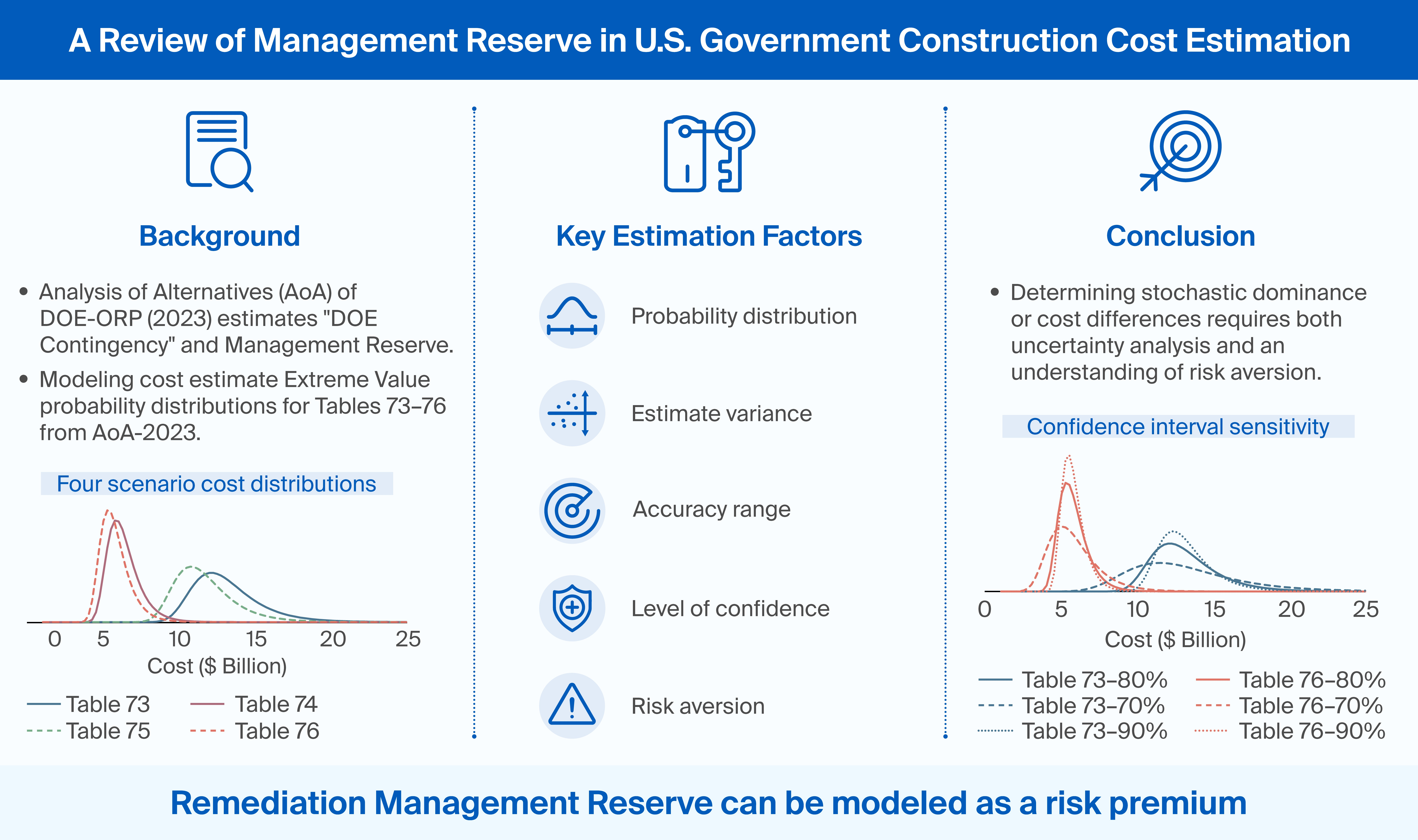
A Review of Management Reserves in U.S. Government Construction Cost Estimation

Abstract

While there is some agreement on estimating construction cost contingency for “known unknowns,” there is little consensus on estimating management reserves for “unknown unknowns.” Definitions of risk and uncertainty also differ between the economics and finance literature and the cost engineering literature. This paper examines how cost engineering guidance on estimating management reserves is applied in government-sponsored project cost estimates. This lack of consensus is evident in a specific program: the management, treatment, and disposal of 212,000 cubic meters of mixed radioactive and hazardous chemical waste generated by plutonium production at the Hanford Nuclear Site. Over $30 billion has been invested in treatment facilities, vitrification plants, and laboratories analyzing gases, liquids, sludges, and salt cake from 177 aging storage tanks. The remaining construction and operating costs are highly uncertain, with estimates ranging from $300 billion to $640 billion. Analyses of alternatives for constructing Hanford waste treatment facilities assume 15% contingencies and 40% management reserves. A method is presented to compute the implicit moments of Extreme Value distributions of cost estimates for different options, helping determine whether one alternative’s cost estimate stochastically dominates others. Adopting industry definitions of contingency and management reserves by federal government agencies could improve construction cost estimation in government-financed programs.

1. Introduction: Estimating “Known Unknowns” and “Unknown Unknowns”

There is an intellectual gap between economics, finance, and other fields regarding the definitions of “risk” and “uncertainty.” This gap makes it difficult to apply modern finance theory to the estimation of a risk-adjusted construction cost. In economics and finance, the consensus definitions of risk and uncertainty are based on Knight’s (1921) work (p. 20; cited at least 36,000 times according to Google Scholar): “The crucial character of the distinction between measurable risk and unmeasurable uncertainty will become apparent in this discussion.” Alhabeeb (2021) writes, “(De Groot and Thurik 2018) reported that 88.3% of articles in this topic, across the related fields, did not adhere to the distinction between risk and uncertainty, rendering all the undesirable theoretical and empirical consequences.”

In everyday language, risk and uncertainty are often framed as “known unknowns” and “unknown unknowns.” Former U.S. Secretary of Defense Donald Rumsfeld (Rumsfeld 2010) famously said (regarding U.S. combat operations in Iraq):

“because as we know, there are known knowns: there are things we know we know. We also know there are known unknowns: that is to say, we know there are some things (we know) we do not know. But there are also unknown unknowns—the ones we don’t know we don’t know …, it is the latter category that tends to be the difficult one.”

Žižek (2006) notes, “In March 2003, Donald Rumsfeld engaged in a little bit of amateur philosophizing about the relationship between the known and the unknown… What he forgot to add was the crucial fourth term, the ‘unknown knowns,’ things we don’t know that we know,” for example, incidents of cognitive dissonance.

Thus, Knightian risk and uncertainty can be expressed in Rumsfeld’s language: risks are known unknowns that can be managed, for example, through diversification (covered by cost contingency and under the funder’s control), while uncertainties are unknown unknowns, covered by management reserve (MR) (Prieto 2021) and under the contractor’s control with funder oversight. Lee et al. (2017):

“Since estimating an MR is difficult because the inherent risks are unpredictable, the traditional percentage method is still used for this purpose. To address this shortcoming, this study proposes an MR estimation method based on the cost and schedule performance ratios of international construction projects.”

This and other papers use empirical data and statistical methods to estimate the costs of unknown unknowns. However, for megaprojects (>$1 billion), the sample is too heterogeneous to support statistical analysis. See Locatelli and Denicol (2024) for a discussion of megaprojects.

On the other hand, GAO (2009, p. 17) and GAO (2020b, p. 13) contradict these interpretations of MR (emphasis added):

“For our purposes in this Cost Guide, contingency reserve represents funds held at or above the government program office for ‘unknown unknowns’ that are outside a contractor’s control… Management reserve funds, in contrast, are for ‘known unknowns’ that are tied to the contract’s scope and managed at the contractor level… The value of the contract includes these known unknowns in the budget base, and the contractor decides how much money to set aside. We recognize that other organizations may use the terms differently.”

(A GAO official verified these definitions in a personal communication on 21 January 2026).

Further, GAO (2018, p. 22) adds, “The cost guide further states that [MR] funds should be included in the budget to cover uncertainties such as unanticipated effort resulting from accidents, errors, technical redirections, or contractor-initiated studies,” i.e., unknown unknowns. As Kwon and Kang (2018) point out,

“Previous studies on this topic have only addressed estimation methods that consider project budget reserves against identified risks [known unknowns]. As a result, project managers still face the challenge of completing projects within given budgets but without the relevant tools to deal with unidentified risks [unknown unknowns]. This study proposes an approach for estimating reserves for both identified and unidentified risks separately. The study also suggests using the three-point estimation technique.”

The three-point estimation technique is a weighted average of (1) optimistic, O, (2) realistic, R, and (3) pessimistic, P, project cost estimates. The three-point “program evaluation and review technique” estimate is [(O + 4R + P)/6], and its standard deviation is [(P − O)/6].

The project management literature and cost engineering literature generally follow the definitions of risk and uncertainty in the Association for the Advancement of Cost Engineering, International (AACEI) recommended practices, RPs (AACEI 2008, p. 2):

“It is AACE’s recommended practice that whenever the term ‘risk’ is used, that the term’s meaning be clearly defined for the purposes at hand… risk means ‘an undesirable potential outcome and/or its probability of occurrence,’ i.e., ‘downside uncertainty (a.k.a. threats).’ Opportunity, on the other hand, is ‘a desirable potential outcome and/or its probability of occurrence,’ i.e., ‘upside uncertainty’… Range estimating is a risk analysis technology that combines Monte Carlo sampling, a focus on a few critical items, and heuristics (rules of thumb) to rank critical risks and opportunities.”

According to the AACEI recommended practices, cost-estimating guidance on contingency and MR for Department of Energy contractors is provided in the DOE Office of Project Management, DOE-OPM (2018a, pp. 51–52):

“This section is compatible with the guidance provided in DOE G 413.3-7A, Risk Management Guide, dated January 2011, for the consistent use and development of Contingency and Management Reserve (MR) in capital asset projects’ cost estimates. Contingency and MR are project cost elements directly related to project risks and are an integral part of project cost estimates… Use of MR should follow [Earned Value Management, EVM, System] rules as per ANSI/EIA-748A.”

On EVM, see GAO (2020b, pp. 207–304). On ANSI/EIA-748 (American National Standards Institute/Electronic Industries Alliance-748), see ASTM International (2017): “Reserve… used to provide insurance against a project or program failing to complete on budget or for the revision of a budget in the case of changed management or program direction and requirement.” AACEI (2020b, Table 1, p. 3) provides a comparison of terms (

Table 1. Translating U.S. government contracting terms into common practice.

Level/Type of Cost	Terms Used in EIA-748/ Capital Programming Guide Reference	Terms Used in Common Commercial Practice
Owner Cost Contingency	Contingency	Management Reserve
Owner Schedule Contingency	Contingency	Schedule Contingency
Contractor Cost Contingency	Management Reserve	Cost Contingency
Contractor Schedule Contingency	Schedule Margin	Schedule Contingency

Source: AACEI (2020b, Table 1, p. 3).

):

To make this literature even more confusing, Hollmann (2022) notes, “One of the more complete treatments of long-range estimates found (in nuclear decommissioning) took” a definitional approach. Hollmann cites NEA and IAEA (2017, p. 15), which introduces new definitions:

“While ‘contingency’ is a commonly used generic term in cost estimation for any financial provision that is above an estimated base cost, contingency may also be given a specific, more limited meaning in particular contexts, for example, in the ISDC [International Structure for Decommissioning Costing]. Therefore, in order to reduce possible ambiguity and confusion, instead of the term ‘contingency,’ the terms ‘estimating uncertainty’ and ‘funded risk’ are used in this report. The term ‘estimating uncertainty’ is used in this report for the provision related to uncertainties within the defined project scope…”

Unfortunately, the term “estimating uncertainty” can be misinterpreted as “estimate uncertainty,” creating confusion. NEA and IAEA (2017, p. 57) illustrates this ambiguity in Table B-3.

Alternative methods for MR estimation have been proposed. For example, Yahia et al. (2020) states, “The [Management Reserve Estimation] model consists of three modules: (1) risk identification, (2) risk uncertainty treatment using a hybrid system that combines fuzzy logic and Monte Carlo simulation techniques, and (3) MR quantification using an integration of Monte Carlo simulation and the expected monetary value. The model has been validated using a real estate development project.”

Given the confusion surrounding definitions of cost contingency and management reserve, and the lack of a literature review on the estimation and use of management reserves in government-financed megaprojects, this paper reviews federal government, project management, and cost engineering guidance on estimating MR. The model introduced in Rothwell (2005) was extended to incorporate risk aversion in Rothwell (2025) and, in Rothwell (2026), further extended to compute confidence intervals for cost contingency estimates. Section 2 reviews the cost engineering literature as interpreted in government cost-estimating guidelines regarding MR. Section 3 reviews MR in construction cost estimates for the remediation of the Hanford Nuclear Site, the U.S. government’s largest environmental liability. Section 4 applies an Extreme Value (Gumbel) statistical model to compute the implied standard deviations of cost estimates, given the assumed contingency and MR rates, enabling tests of implicit statistically significant differences between alternative cost estimates. Section 5 discusses these results, offers conclusions, and suggests future research.

2. A Review of Federal and Industry Management Reserve Guidelines

According to GAO (2025), the five U.S. federal departments with the highest contractor funding are the Department of Defense ($445 billion in Fiscal Year, FY, 2024; the largest program is the missile defense system, with a $151 billion ceiling over 10 years), the Department of Veterans Affairs ($67 billion; the largest construction project is the Louisville Medical Center, at $970 million), the Department of Energy ($48 billion; the largest program is the cleanup of the Hanford Site outside Richland, Washington, estimated to cost at least $300 billion), the Department of Health and Human Services ($37 billion, of which less than $10 billion was spent on construction projects in FY 2024), and the General Services Administration ($27 billion, with $1.8 billion in direct investments in new construction and federal building repair and alteration projects).

The majority of contracts in both the military and civilian sectors are awarded through market competition (“competed”), and the majority of competed and non-competed contracts are fixed-price, as GAO (2020b, p. 230) notes:

“Research has found that programs typically set their contract value so they can set aside 5 to 10 percent as a management reserve. This amount may not be sufficient for some programs and may be more than others need. One way to derive the amount of management reserve needed is to conduct a risk analysis for schedule (to determine the schedule reserve needed) and for cost (to determine the management reserve for cost). Risk and uncertainty analysis should be used to specify the probability that work will be performed within budget. The likelihood of meeting the budget can then be increased by establishing a sufficient management reserve budget.”

Department of Defense (DOD) cost estimators and contractors rely on DOD (2022), GAO (2020b), and U.S. Army Corps of Engineers (USACE) guidelines. (Much of the DOD guidance is available through the Defense Acquisition University (https://www.dau.edu), which requires trainee registration to access it). DOD (2022, p. 20) discusses risk and uncertainty:

“Analysts often use the terms risk and uncertainty interchangeably. In fact, they are distinct from one another. Uncertainty is the indefiniteness of the outcome of a situation. Uncertainty captures the entire range of possible positive and negative outcomes associated with a given value or calculated result. In a cost estimating model, an analyst generally addresses uncertainty first. The analyst then addresses risks/opportunities if and only if the uncertainty assessment has not already captured them.”

Christensen and Templin (2000) analyzed the use of MR in DOD contracts:

“This paper provides [an analysis of] the amount and use of MR budget on hundreds of defense acquisition contracts from 1975 to 1998. Results indicate statistically significant differences in the median MR budget percentage across contract types (cost-reimbursable and [fixed-]price) and the military services managing the contracts (Army, Air Force, Navy).”

Further, USACE (2020, p. A-9-3) states, “Planning, pre-concept, concept, and final design cost estimates shall be thoroughly documented to explain the basis of the estimate and to include contingencies associated with any unknowns or risk factors.” However, these documents neither define MR nor specify how to estimate it.

The Department of Veterans Affairs (VA) also relies on USACE. According to GAO (2017), “the VA has 26 ongoing medical-facility construction projects… [T]his report assesses… opportunities for improvements in managing these projects, particularly VA’s medical facility in Denver, the only project outsourced to USACE that is under construction.” GAO (2017, p. 22):

“A cost estimate is considered credible when any limitations of the analysis are discussed, and the estimate’s results are cross-checked. We found USACE’s estimate substantially meets this characteristic. A formal cost risk and uncertainty analysis was performed, and it was used to set the amount needed for cost contingency for the program.”

However, GAO (2017, p. 26) states, “Contingency is a reserve of extra time to account for known and quantified risks and uncertainty,” i.e., known unknowns, which appears to contradict GAO (2009, p. 17) and GAO (2020b, p. 13), as quoted above.

In general, the Department of Health and Human Services (HHS) follows the GAO cost-estimating guidelines and General Services Administration (GSA) reporting regulations (GSA 2025). HHS-specific guidance is provided in HHS (2025). Guidance on determining contingency, but not management reserve, is available in GSA (2022). Robert-Santiago et al. (2024) explain, “Contingencies should be determined by the level of risk in a project. Currently, GSA uses 7% for new Capital Construction and 10% for [repair and alteration] work. This might change in the future if we successfully deploy a Risk-Based Contingency Model,” e.g., as proposed in Ordóñez and Park (2011).

For projects funded by the U.S. Department of Energy (DOE), cost-estimating guidance on risk and uncertainty analysis is provided in DOE-OPM (2018a) and DOE-OPM (2021). The DOE Cost Estimating Guides describe how to estimate project costs in accordance with GAO (2009): “An independent cost review is a vital step in providing consistent, professionally prepared cost estimates (Step 7, GAO 12 Key Steps Development Process, GAO (2009)).” DOE-OPM (2021, p. 11.1) discusses confidence levels for cost contingency and MR, stating, “At a minimum, project performance baselines should be estimated, budgeted, and funded to provide a range of 70–90 percent [P70 to P90] confidence level for DOE capital asset projects.”

DOE-OPM (2018a, p. 61) notes, “One approach to account for estimate uncertainty is to use uncertainty ranges established by professional societies such as AACE International [AACEI].” (These “uncertainty ranges” are likely AACEI “accuracy ranges.”) Each DOE Cost Estimating Guide includes AACEI Recommended Practice No. 18R-97 as an appendix. DOE-OPM (2018b, p. 54) also states:

“The DOE Contingency discussed here is the contingency needed to mitigate project risks that are within the project baseline but are generally beyond the contractor’s control. It is additive to the MR... The steps to follow for DOE Contingency are similar as for MR.”

Regarding total contingency, DOE-OPM (2021, p. 54) states, “Add the cost contingency (derived from the risk analysis) to the cost estimate uncertainty contingency, at the same confidence levels, to derive the total MR for the contractor.”

Table 2. AACEI (2020a). Estimate classes and accuracy ranges.

Estimate Class	Estimate Designation	AACEI Low-End Accuracy Range	AACEI High-End Accuracy Range	Narrow Accuracy	Wide Accuracy
5	Conceptual Screening	−50% to −20%	+30% to +100%	−20% to +30%	−50% to +100%
4	Feasibility Study	−30% to −15%	+20% to +50%	−15% to +20%	−30% to +50%
3	Budget Authorization	−20% to −10%	+10% to +30%	−10% to +10%	−20% to +30%
2	Control or Bid	−15% to −5%	+5% to +20%	−5% to +5%	−15% to +20%
1	Check Estimate	−10% to −3%	+3 to +15%	−3% to +3%	−10% to +15%

Source: based on AACEI (2020a, Table 1).

presents cost estimate classes, project stages, and accuracy ranges, based on AACEI (2020a).

DOE-OPM (2019, pp. 2–3) discusses confidence levels for project cost approvals:

“When the Office of Project Management (PM) completes an independent cost review (ICR) or an independent cost estimate (ICE) report, the team often refers back to [AACEI (2020a, Table 1)] to determine the estimate class, and based on the estimate class determination, it assigns expected estimate uncertainty ranges.”

However, DOE-OPM (2018a, p. 64) warns, “It should be cautioned that the recommended contingency levels in these documents do not provide a basis for the recommended confidence levels (70–90 percent [P70 to P90]) in this Guide for the derivation of contingency and management reserve by quantitative risk analysis.”

The DOENational Nuclear Security Administration (DOE-NNSA) follows guidance similar to that of DOE-Environmental Management (DOE-EM). In DOE-CF (2025, p. 538), regarding the design and construction of the Naval Reactors Facility Project in Idaho:

“The cost range approved with CD-1 [Critical Decision 1: Approve Alternate Selection and Cost Range] is $1,630,000,000 to $5,000,000,000 (then-year dollars). The point estimate associated with the current stage of the project (conceptual design) is $3,228,500,000 (then-year dollars). The management reserve and government contingency included in the cost estimate provides approximately 80% confidence [P80] in the project cost.”

In contrast, other DOE offices hold different understandings of contingency and MR. For example, DOE-LM (2023, p. 79), which manages historic sites and remediation projects, states, “The methodology used for calculating management reserve, otherwise known as contingency dollars for each site, is documented within the appropriate risk register.”

Federal government and industry guidelines do not distinguish between cost-uncertainty analysis for estimating contingency funds under the program office’s control (known unknowns at the time of contract signing) and management reserve funds under the contractor’s control (unknown unknowns at the time of contract signing). An interpretation of the guidance suggests that either both contingency and MR cover “known unknowns” but are controlled by different parties, or that contingency covers “probable unknowns” and MR covers “improbable unknowns.” The government cost-estimating guidance is unclear about whether management reserves are intended to ensure against “known unknowns” or “unknown unknowns.” This confusion is evident in the extremely high and uncertain cost estimates for the Hanford Nuclear Site cleanup.

3. A Review of Management Reserves in Hanford Cost Estimates

Hanford remediation is the U.S. federal government’s largest environmental liability. DOE-RL (2019, p. 2.6), Table 2.2, “Hanford Site Remaining Cleanup Cost Estimated Ranges by [Project Baseline Summary] (Billions $),” reports “Total Remaining Estimated Costs $323.2–$677.0.” The Hanford cleanup is the responsibility of DOE-EM’s Hanford Field Office (DOE-HFO), formed in October 2024 by merging the Office of River Protection (DOE-ORP) and the Richland Operations Office (DOE-RL).

DOE-HFO oversees the management and disposal of approximately 212,000 cubic meters (56,000,000 gallons) of mixed waste, including gases, liquids, sludges, and salt cake, that contain dozens of radioisotopes and hazardous chemicals. (See Invernizzi et al. 2020 for comparison with other nuclear site decontamination and demolition, D&D, projects). It is estimated that 90% of this waste is Low Activity Waste (LAW). This waste, stored in 177 single- and double-shell tanks, was generated during the reprocessing of spent nuclear fuel to produce weapons-grade plutonium (Silverio and de Queiroz Lamas 2011). The Pacific Northwest National Laboratory (PNNL) provided an assessment of Hanford remediation for the DOE-RL in Wood et al. (2001, p. 1.2):

“The sheer expanse of the Hanford Site [1518 square km or 586 square miles], the inherent hazards associated with the significant inventory of nuclear materials and wastes, the large number of aging contaminated facilities, the diverse nature and extent of environmental contamination, and the proximity to the Columbia River [the largest river in the Western Hemisphere flowing into the Pacific Ocean] make the Hanford Site perhaps the world’s largest and most complex environmental cleanup project.”

Andrews (2015) suggests that project complexity depends on lifecycle size and duration, Technology Readiness Levels, risk (as described in DOE-OPM 2021), and regulatory requirements.

As noted in DOE-RL’s (2011) Hanford Lifecycle Scope, Schedule and Cost Reports (p. ES-1), “The 2011 Lifecycle Report [LCR] is based on scope, schedule, and cost estimate information and incorporates regulatory milestones from the Consent Decree [settling State of Washington v. Chu] and TPA [Tri-Party Agreement] Settlement Package that became effective 25 October 2010.” The three parties to the TPA are the DOE-EM, the Environmental Protection Agency (EPA), and the Washington State Department of Ecology. The TPA was initially signed in 1989, amended multiple times (DOE-HFO 2025b), and updated in 2025 (Ecology 2025).

Table 3. Hanford remediation accounts and base costs, Tables D-02 to D-12, DOE-RL (2019).

Table	Account	Base Cost (Billions)	Title
D-02	RL-0013C	$9.40	Solid Waste Stabilization and Disposition—200 Area
D-03	RL-0020	$10.10	Safeguards and Security
D-04	RL-0030	$7.90	Soil and Water Remediation—Groundwater
D-05	RL-0040	$13.70	Nuclear Facility D&D—Remainder of Hanford
D-06	RL-0041	$1.40	Nuclear Facility D&D—River Corridor Closure Project
D-07	RL-0042	$0.70	Nuclear Facility D&D—Fast Flux Test Facility Project
D-08	RL-0100	$1.07	Richland Community and Regulatory Support
D-09	RL-0201	$20.40	Hanford Sitewide Services
D-10	RL-LTS	$12.22	Long-Term Stewardship
D-11	ORP-0014	$213.90	Radioactive Liquid Tank Waste Stabilization and Disposition
D-12	ORP-0060	$15.50	Major Construction—Waste Treatment Plant (WTP)
Total	Base Cost	$306.29

Source: DOE-RL (2019, Appendix D); these values were not updated in later LCR reports.

lists the projects in the Hanford remediation program.

Rothwell (2026) models cost contingency estimates for a specific construction project in the DOE-HFO portfolio under the DOE-EM account ORP-0060 (GAO 2023): the Waste Treatment Plant (WTP). The WTP includes the High-Level Waste (HLW) facility, the Pre-Treatment (PT) facility, the Direct-Feed Low Activity Waste (DFLAW, GAO 2022) system, the Analytical Laboratory (LAB), and the Balance of Facilities (BOF, including the Tank-Side Cesium Removal, TSCR, facility).1

The DFLAW complex was not part of the original program to meet the TPA requirements. Construction of the original WTP began in 2000, but by 2012, significant technical uncertainties had emerged regarding HLW and PT technologies. In response, DOE-EM shifted its focus to vitrifying LAW by constructing the LAW-Vit plant and associated facilities and infrastructure.2 The TSCR facility was built between 2019 and 2021 by Washington River Protection Solutions (WRPS, owned by Amentum and BWX Technologies, BWXT) and has operated since 2022 (Marcial et al. 2024). DOE-EM (2023) stated, “The team completed TSCR construction and started operations three months ahead of schedule and $29 million under the approved total project cost of $164 million.” Regarding the DFLAW system cost, GAO (2022) noted, “DOE estimates that it will complete the work to start DFLAW operations by 31 December 2023, at a cost of approximately $8.3 billion.”

Bechtel National, Inc. (BNI) is the prime contractor responsible for designing, constructing, and commissioning the WTP, including DFLAW. Hanford Tank Waste Operations and Closure, LLC (H2C, a joint venture of Amentum, BWXT, and Fluor) began vitrifying LAW in October 2025 (ANS 2025a).

Table 4. The Direct-Feed Low Activity Waste (DFLAW) complex.

Facility	Function
Tank Farm	Double-shell Tank AP-107 collects and transfers liquid waste to TSCR
TSCR	Filters cesium, strontium, and suspended transuranic solids from liquid waste
IXC	Ion Exchange Column (IXC) stores waste removed by TSCR
HLW-Vit	The High-Level Waste Vitrification facility will vitrify waste from IXC and ETF
Tank Farm	TSCR-treated LAW is stored in Tank AP-106 and transferred to the LAW-Vit Facility
222-S Lab	Provides analytical services for Tank Farms and LAW-Vit feed qualification
LAW-Vit	Mixes LAW with glass-forming materials in two high-temperature melters
EMF	Concentrates liquid secondary waste from LAW-Vit through evaporation
ETF	Treats concentrated liquid from EMF and other sources to remove contaminants
LAB	Provides laboratory services to confirm that the LAW-Vit Facility is operating properly
ILAW-Trans	Transports ILAW glass-filled containers from LAW-Vit to the IDF
IDF	Accepts containers of vitrified LAW for disposal and other solid LAW waste forms
BOF	Provides essential services to support DFLAW system operations
Infrastructure	Provides electricity, water, sewage, security, emergency, and IT services, and roads

Notes: AP refers to the newest 4200-cubic-meter (1,000,000-gallon) double-shelled tanks at the Hanford tank farm, constructed between 1982 and 1986; ILAW is Immobilized LAW; and IDF is the Integrated Disposal Facility (~1,500,000 m³). Source: DOE-HFO (2024).

lists the DFLAW subsystems. H2C operates under an Indefinite Delivery/Indefinite Quantity (IDIQ) contract with a maximum value of $45 billion over 10 years (DOE-EM 2024). (CRS 2024, defines “an IDIQ contract as one that provides for an indefinite quantity, within stated limits, of supplies or services during a fixed period”). HLW will be stored onsite until the HLW vitrification facility (HLW-Vit in Table 4) is completed, as mandated by 2033. It will then be vitrified and shipped to a geologic repository, such as the Waste Isolation Pilot Project (WIPP) in New Mexico.

Regarding Hanford remediation, the Project 2025 Advisory Board (2023, p. 395) proposed,

“The Hanford site in Washington State is a particular challenge. The [TPA] has hampered attempts to accelerate and innovate the cleanup. A central challenge at Hanford is the classification of radioactive waste. High-Level Waste (HLW) and Low-Level Waste (LLW) classifications drive the remediation and disposal process… changes in waste classification from HLW to LLW… would allow LLW to be grouted rather than vitrified.”

On the use of grouting instead of vitrification, see Bates et al. (2023) and Stang (2025).

In DOE-CF (2017, p. 87), spending in the WPT account (ORP-0060: Major Construction—Waste Treatment Plant) from 1997 to 2016 totaled $10.2 billion, with projected lifecycle costs in the “low range” of $11.2 billion and the “high range” of $11.2 billion, implying a remaining cost of $1 billion. In DOE-CF (2024, p. 39), expenditures from 1997 to 2023 reached $14.8 billion, with a projected total lifecycle cost from FY 2024–2091 in the “low range” of $30.2 billion and the “high range” of $31.6 billion (melters will need to be replaced periodically). Thus, the remaining cost was estimated to be between $15.4 billion and $16.8 billion, requiring more spending than what had already been spent. The estimated cost of the “Radioactive Liquid Tank Waste Stabilization and Disposition” project (account ORP-0014) increased from a total cost between $53 billion and $61 billion in DOE-CF (2017, p. 87) to between $178 billion and $329 billion in DOE-CF (2024, p. 39), i.e., with additional spending of between $165 billion and $316 billion.

Estimating Hanford remediation costs is challenging because the mission is a large-scale Research, Development, Demonstration, Decontamination, and Demolition (RDDD&D) project. As Alexander (2018, pp. vii–viii) explains,

“Design, performance, or technical requirements, which drive traditional parametric models or translate analogous system costs, are often unavailable in the early life-cycle stages of basic or applied technology development… Researchers have proposed or developed frameworks, analyses, and modeling concepts that apply predictors such as Technology Readiness Levels (TRLs).”

TRLs are outlined in DOE-OPM (2015) and GAO (2020a, Appendix VIII): TRL-1 is “basic principles reported,” TRL-4 is “laboratory validation,” TRL-7 is “prototype demonstration,” and TRL-9 is “successful mission operation.” In other words, “Research” spans TRL-1 through TRL-3, “Development” includes TRL-4 and TRL-5, “Demonstration” spans TRL-6 through TRL-8, and “Deployment” occurs at TRL-9. Fraizinger (2019) discusses the relationships between the estimate classes in Table 2 and TRLs. However, the literature linking TRL levels to cost contingencies or management reserves is limited.

DOE-RL provided estimates of Hanford remediation costs, along with an uncertainty analysis to determine contingency and MR, for the Hanford Lifecycle Scope, Schedule and Cost Reports (LCRs). DOE-RL (2011, p. E-10), “Table E-6. [Spent Nuclear Fuel] Stabilization and Disposition ([Project Baseline Summary] RL-0012) Near-Term Schedule and Costs, Level 3, by Fiscal Year ($1000, Escalated),” projected a total D&D spending for the K Basin, including the area known as “K West,” at $571,600,000, with 12% ($68,800,000) allocated to “Cost and/or Schedule Uncertainty” and 19% ($107,520,000) to “Management Reserve–Basins Operations and Maintenance.” (According to Prieto (2021), “Typically, management reserves for large, long-duration projects tend to fall within the 5–15 percent range, dependent on project complexity.”).

DOE-RL (2022) summarizes the 2019 LCR results in Table 2.2, “Hanford Site Remaining Cleanup Cost Estimated Ranges by [Project Baseline Summary],” for ORP-0060, with estimated construction costs ranging from $19.6 billion to $31.1 billion (DOE-RL 2022, p. C-69). The report notes that “Cost ranges are shown in this table to reflect cost and schedule uncertainty; the lower number is used throughout this report.”

DOE-RL (2013, p. D-1) states, “cost and/or schedule uncertainty [is] also referred to as contingency.” In the 2011 and 2012 LCRs, MR was reported for various accounts, whereas from 2013 to 2015, MR was combined with contractor fees.3 In DOE-RL (2014, Table 3-2, p. 3.5), the MR category includes “contractor’s fee, management reserve, and Government & Administrative allocations.” In Table 3-3, “[Usage-Based Services], [General and Administrative], and Direct Distribution” includes the contractor’s fee and management reserve. DOE-RL (2022, p. 1.12) describes management reserve:

“Cost and schedule uncertainty are included in the development of Total Project Cost and… are reserved to accommodate additional work scope related to risk events that may occur from conditions and events that were not known during project planning and other unanticipated changes or uncertainties [unknown unknowns]. This includes estimates for cost and schedule uncertainty based on risk analysis methods that comply with DOE guidelines and orders.”

This text was revised in DOE-HFO (2025a, p. 1.12): “Quantitative risk analysis is used to estimate the impact of estimation uncertainty and risks in terms of joint cost and schedule, as outlined in the Cost Estimating and Assessment Guide.”

DOE-RL (2022) does not provide an uncertainty analysis for any account. Additionally, in the most recent LCR (DOE-HFO 2025a, p. v), the estimated construction cost for ORP-0060 is between $10.1 billion and $20.3 billion: “The contingency for the [WTP] is contained within the total project cost; the high-range includes the Pretreatment Facility.” However, there is no explanation of the origins of these values, nor is there an uncertainty analysis, as in DOE-RL (2019). Moreover, DOE-HFO (2025a, p. 1.12) might confuse “estimate uncertainty” with “estimating uncertainty” as in NEA and IAEA (2017): “Estimating uncertainty refers to the fact that because a cost/schedule estimate is a forecast, the actual cost/schedule will likely differ from the original base estimate.”

Also, there are the Analysis of Alternatives (AoAs). DOE-ORP (2023, p. 159) states,

“To accommodate the possible deficiencies identified by the [Office of Project Management] review of the USACE parametric analysis (USACE 2018), the AoA estimate includes slightly higher allowances for MR and DOE Contingency than those used by USACE. The adders included by the AoA Team are 40% (compared to 36.3% by USACE) and 15% (compared to 13.4% by USACE), respectively, for MR and DOE Contingency.”

Although DOE-ORP (2023) did not conduct a quantitative risk analysis, it identified uncertainties stemming from the limited technological readiness of Hanford vitrification technologies (DOE-ORP 2023, p. 4; on vitrification technologies, see Goel et al. 2019; ANS 2025b):

“(DOE-OPM 2018b) requires that critical technologies for Major System Acquisition (MSA) projects achieve Technical Readiness Level TRL-4 prior to [Approval of the Alternative Selection and Cost Range]… (DOE-OPM 2018b) also requires that all critical technologies achieve TRL-7 prior to [the Approval of the Performance Baseline]. Given the difficulty that DOE has had in resolving the [issues] associated with the new tank mixing technologies for the WTP PT Facility, the AoA Team will not evaluate HLW processing alternatives that use critical technologies that have not been demonstrated for HLW processing.”

The lack of transparency regarding MR use prompted a DOE-OIG audit of a Hanford contractor. DOE-OIG (2017, p. 3) states,

“During the course of the audit, we held discussions with the [OPM] concerning the proper use of management reserve, and the unique facts and circumstances associated with the Sludge Removal Project. The [OPM] agreed that the use of management reserve to reset the baseline for already completed work scope would, under normal circumstances, be noncompliant with the American National Standards Institute 748-C Earned Value Management Intent Guide.”

DOE-OAM (2014) stated, “Burden of proof is on the contractor to demonstrate it is an authorized use [of MR].” Given conflicting guidance on whether MR covers “measurable risks” or “unmeasurable uncertainties,” there is confusion at Hanford about how to estimate and apply MR. In fact, Hanford cost estimators calculate contingency and MR in the same way; they simply add them together under the heading “Cost and Schedule Uncertainty.” When combined, what might be the implicit probability distributions of the resulting construction cost estimates?

4. A Method of Determining the Implicit Statistical Significance of Differences in Cost Estimates

Does the estimation of MR in Hanford remediation cost estimates follow DOE guidelines? DOE-ORP (2023, pp. 161–164), i.e., AoA-2023, presents “DOE Contingency” and MR for various Hanford cleanup scenarios.

Table 5. Estimated total spending plan to complete HLW with and without the PT Facility.

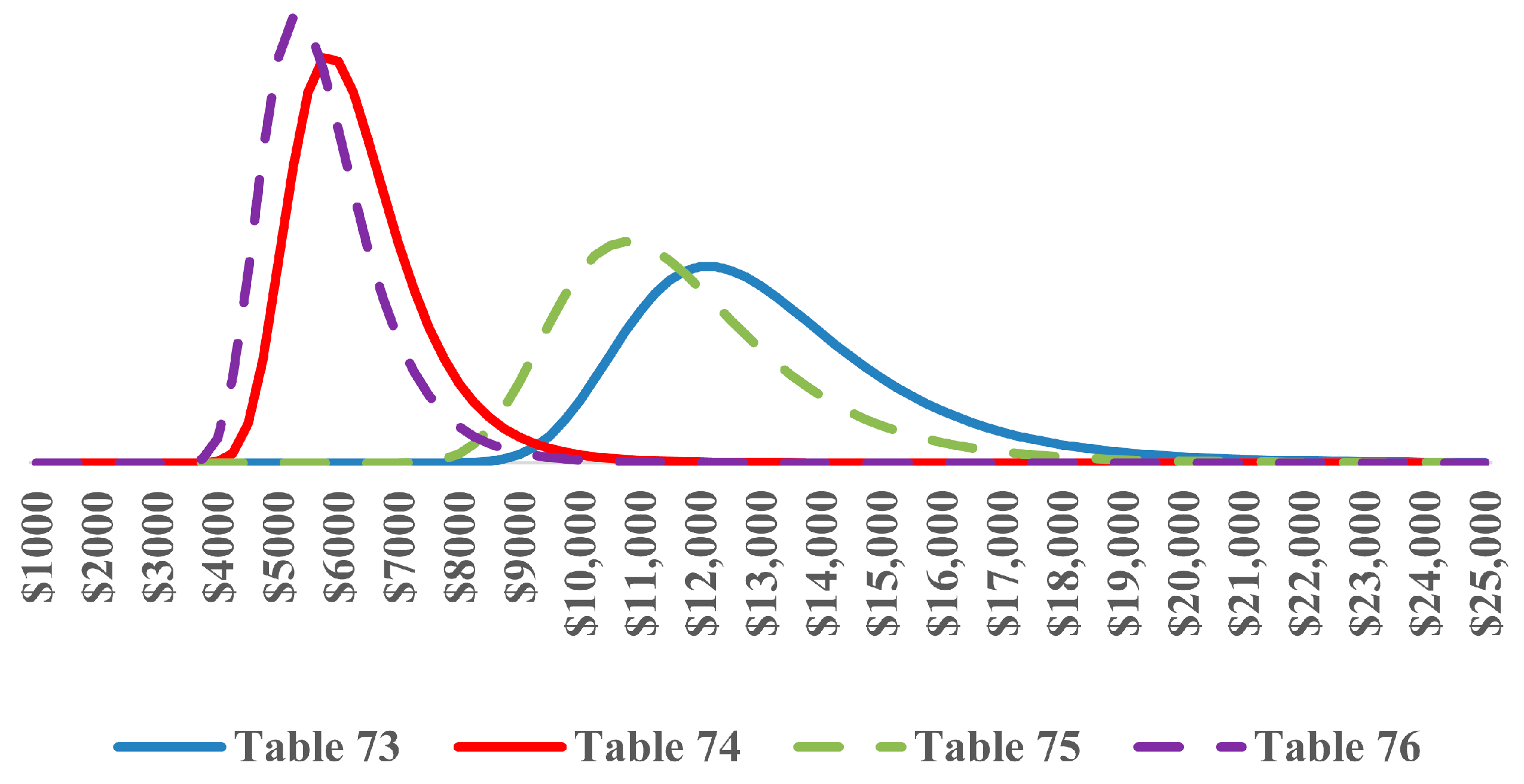
	Table 73	Table 74	Table 75	Table 76
	Base Case:	HLW	HLW and	Minimal Direct Feed
	HLW and PT	Completion	Re-Purposed	HLW Completion
	Completion	Only (No PT)	PT	Only (No PT)
Element	(In Millions)	(In Millions)	(In Millions)	(In Millions)
PT	$3569	$0	$2904	$0
HLW	$1829	$1829	$1829	$1829
Melter	$68	$68	$68	$0
BOF	$180	$162	$180	$146
LAB	$100	$90	$100	$81
Added Scope: DFHLW	$0	$480	$0	$318
Project + Facility Services	$2422	$1116	$2151	$1006
ORP Direct Support	$330	$330	$330	$330
Base Costs	$8497	$4074	$7561	$3708
Escalation	$3904	$1906	$3470	$1739
Escalation %	45.95%	46.78%	45.89%	46.89%
Fee	$729	$352	$649	$320
Fee%	5.88%	5.88%	5.88%	5.88%
Escalated Base Cost	$13,130	$6332	$11,679	$5767
MR%—Fee	40.0%	40.0%	40.0%	40.0%
MR	$4960	$2392	$4412	$2179
CON%—Fee	15.0%	15.0%	15.0%	15.0%
DOE Contingency	$1860	$897	$1655	$817
Total	$19,951	$9621	$17,746	$8763

Notes: PT is the Pre-Treatment Facility; HLW is the High-Level Waste Facility; the melter mixes molten glass-making materials, such as silica, with radioactive and hazardous chemical waste at 1150 °C; BOF is the Balance of Facilities; LAB is the Analytical Laboratory; DFHLW is a Direct-Feed High-Level Waste Facility; ORP is the Office of River Protection (a precursor to HFO); and CON% is the cost contingency percentage. Source: DOE-ORP (2023, pp. 161–164).

summarizes Tables 73–76 from AoA-2023. (The contractor’s fee is excluded from calculations of MR or contingency values). The values of 15% for DOE Contingency and 40% for MR are based on USACE (2018), as cited in DOE-ORP (2023, p. 159). However, AoA-2023 did not conduct a probability analysis because the values for DOE Contingency and MR are identical across alternatives. (One would expect MR to be lower in alternatives without a PT because they would be less complex). Without an uncertainty analysis, DOE-HFO cannot determine which alternative is (first-order) stochastically dominant (Wolfstetter 1996).

A Monte Carlo simulation yields an expected mean cost estimate, CE, and a standard deviation, SD, for a given probability distribution. (Rothwell (2025) reconstructs a Monte Carlo simulation of the Work Breakdown Structure (WBS) for the decommissioning cost of the Kewaunee Nuclear Power Plant, yielding an expected cost and a standard deviation; this entails assigning a cost and a probability distribution to each input for every task in the WBS). Equation (1) in Rothwell (2025) defines the contingency rate, CON%, as a function of (1) the ratio of the standard deviation to the expected cost, (2) a multiplier that “stretches” the ratio to cover a specified accuracy range (see Figure 1 in Rothwell (2026)), and (3) a measure of Absolute Risk Aversion (ARA):

CON% = (SD/CE) ∙ [80%-Interval] ∙ ā,

(1)

where the [80%-Interval] multiplies the (SD/CE), so that the result covers 80% of the accuracy range, and ā is the Absolute Risk Aversion constant, with ā > 0 (Rothwell 2016, p. 120; Rao 2020).4 However, if the contingency rate is known and (SD/CE) is unknown, one can solve for (SD/CE) as a function of CON%:

(SD/CE) = CON%/([80%-Interval] ∙ ā).

(2)

The probability distribution and density of the cost estimate can be modeled using closed-form, skewed Extreme Value (Gumbel) functions (Johnson et al. 1995, p. 2):

F(x) = exp {−exp (−A)},

(3)

f(x) = (1/b) · exp (−A) · F(x),

(4)

A = (x − m)/b, where b > 0, and

(5)

P(x) = m − b · ln {−ln[F(x)]},

(6)

where m is the mode (a “shift” parameter) and b (a “scale” parameter) equals [SD · (6^½/π)] ≈ SD · 0.78. The mean is approximately [m + (b · 0.577)] from Johnson et al. (1995, p. 17). The median (P50) is [m − (b · ln(−ln(0.5))] ≈ [m + (b · 0.3665)] from Johnson et al. (1995, p. 13). Thus, mean > median > mode, P(80) equals {m − b · ln [−ln(0.8)]} ≈ [m + (b · 1.5)], and P(95) ≈ [m + (b · 2.97)].

Assuming CON% is 55% from

Table 6. Estimated extreme value parameters for total spending plans (in order of decreasing cost).

Element	Table 73	Table 75	Table 74	Table 76
Mean = CE	$13,130M	$11,679M	$6332M	$5767M
MR% + CON%	55%	55%	55%	55%
SD = (55%/2.4) × CE	$3009M	$2677M	$1451M	$1322M
b = SD × 0.78	$2347M	$2088M	$1132M	$1031M
mode = CE − (b × 0.577)	$11,776M	$10,475M	$5679M	$5173M
median = m − (b × 0.577)	$12,879M	$11,456M	$6210M	$5657M
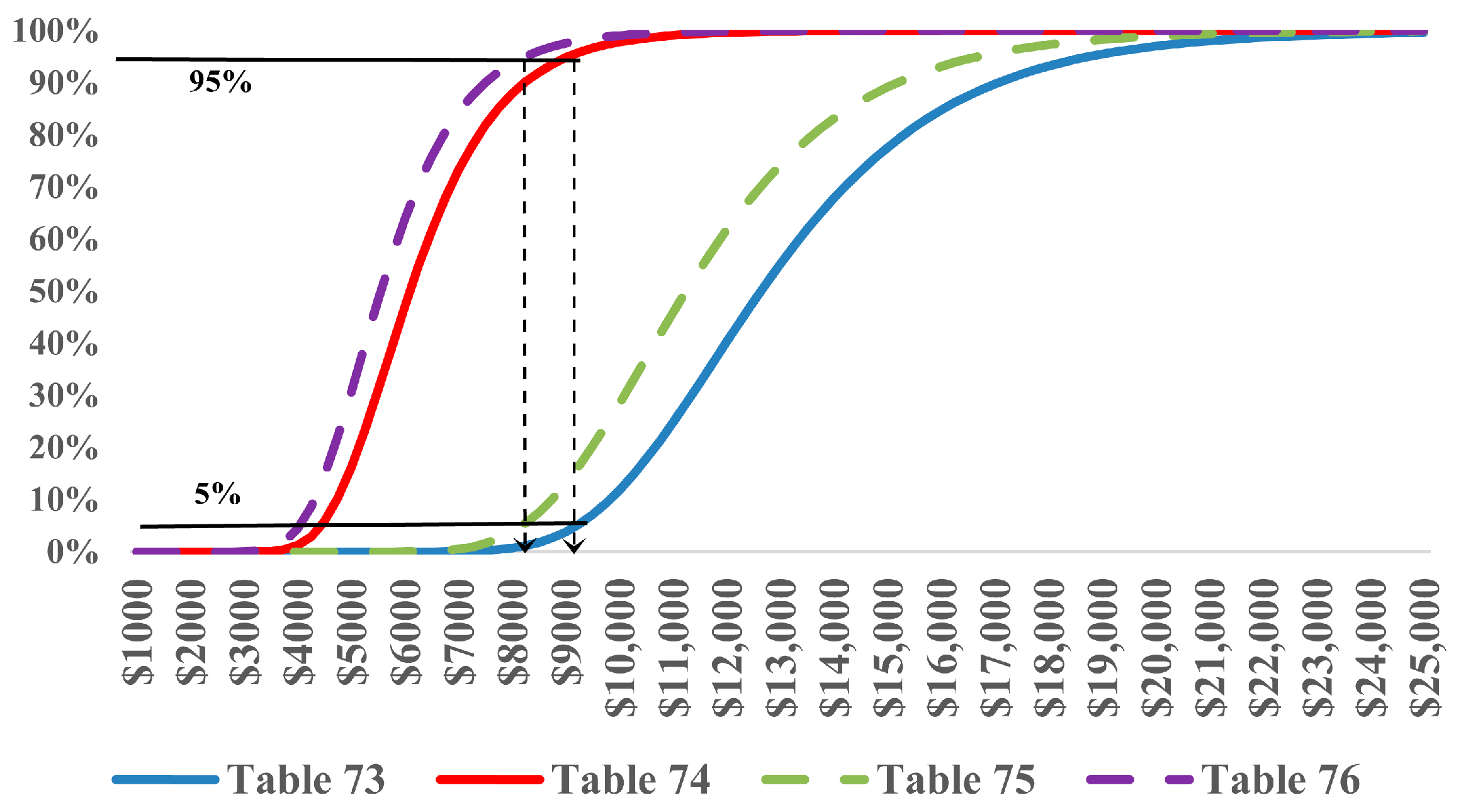
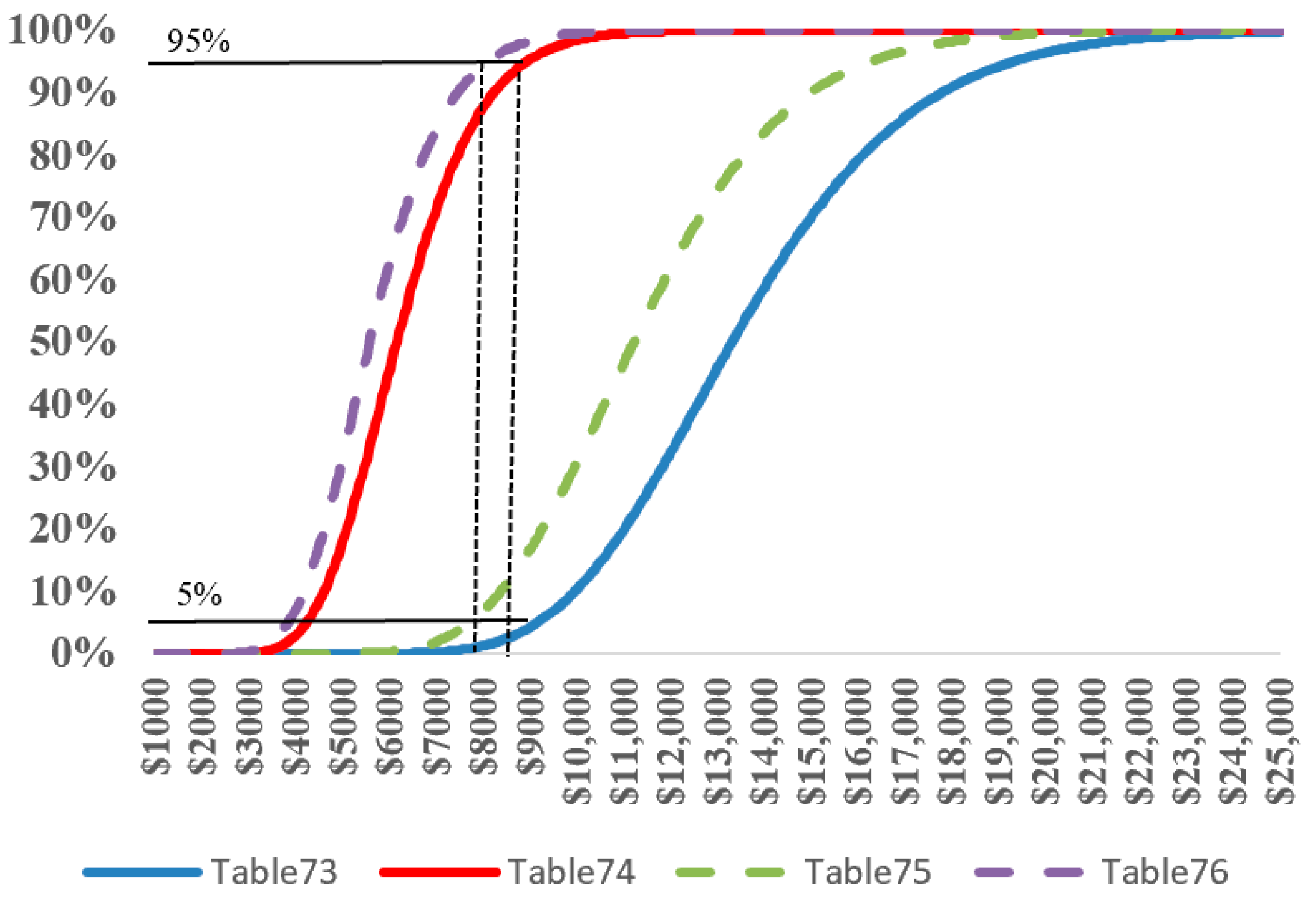
5% with CI-70 (=P85 − P15)	$8218M	$7310M	$3963M	$3610M
95% with CI-70 (=P85 − P15)	$20,151M	$17,925M	$9717M	$8852M
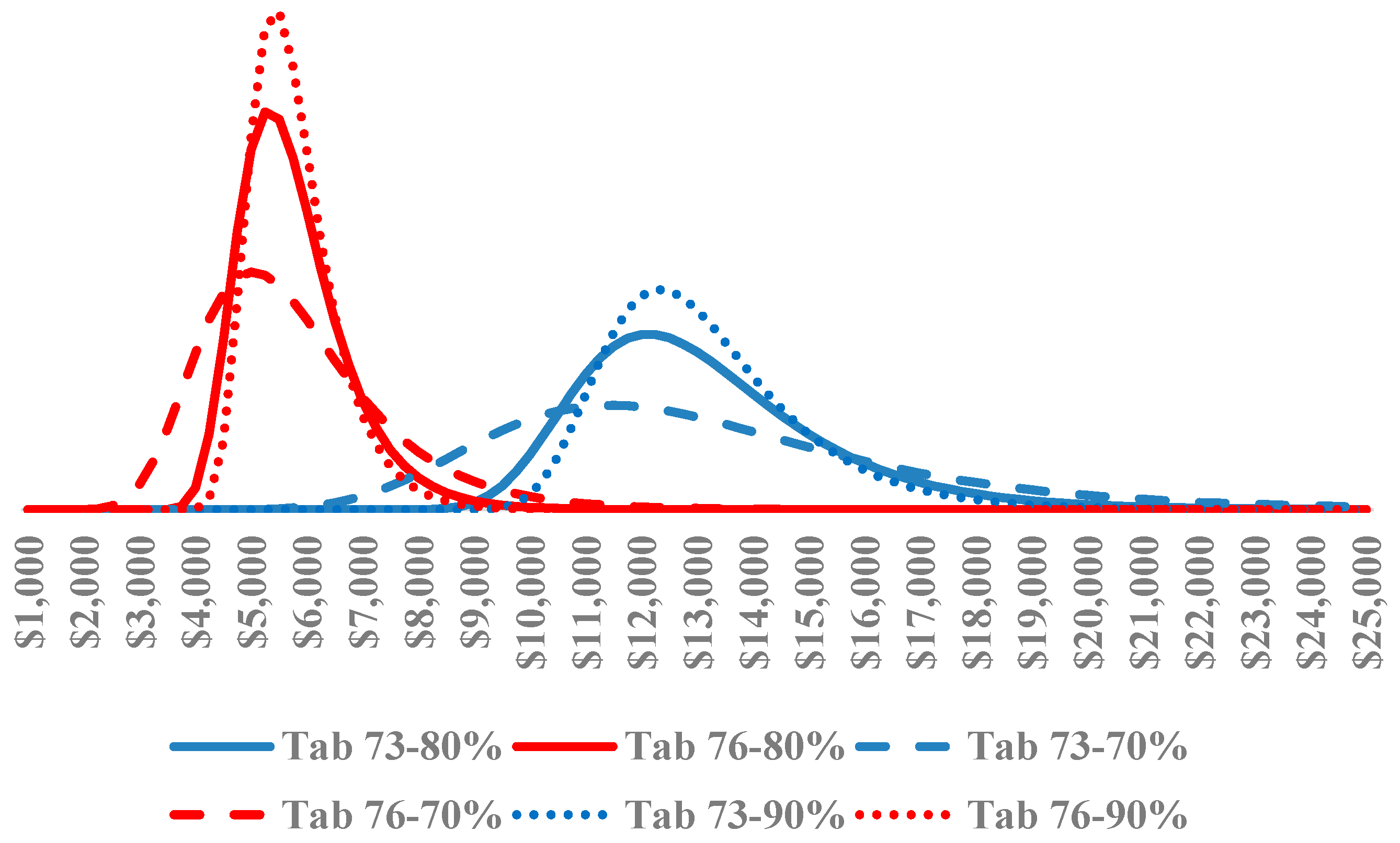
5% with CI-80 (=P90 − P10)	$9201M	$8184M	$4437M	$4042M
95% with CI-80 (=P90 − P10)	$18,747M	$16,676M	$9040M	$8235M
5% with CI-90 (=P95 − P5)	$10,805M	$9611M	$5210M	$4746M
95% with CI-90 (=P95 − P5)	$16,454M	$14,636M	$7934M	$7227M

Notes: CE is the expected cost; MR% is the management reserve percentage; CON% is the cost contingency rate; SD is the standard deviation; b and m are Extreme Value parameters; and CI is the confidence interval. Source: Equations (2)–(6).

, [80%-Interval] is 2.4 from Rothwell (2025, Section 4), and risk neutrality (ā = 1 for an 80% confidence interval), Table 6 presents the implicit parameter values. Figure 1 shows the resulting probability densities. It is apparent that “Base Case: HLW and PT Completion (Table 73)” is similar to “HLW and Re-Purposed PT (Table 75),” and that “HLW Completion Only (no PT) Table 74” is similar to “Minimal Direct Feed HLW Completion (no PT) Table 76,” as shown in Table 6, where the columns from Table 5 have been ordered by total cost.

Further, as shown in Figure 2 and using Equation (6), (1) the alternative in Table 73 is significantly different from the case in Table 74 (95% of the distribution exceeds $9040M, placing it in the highest 5% of the distribution in Table 74) and (2) the alternative in Table 75 is significantly different from the case in Table 76 of the distribution in Table 75 (94.6% of the distribution exceeds $8235M, where {$8235M = $10,475M − [$2088M · (ln(−1 · ln(0.0537)))]}, placing it in the highest 5.4% of the distribution in Table 75). The alternatives in Tables 74 and 76 stochastically dominate those in Tables 73 and 75, respectively, i.e., are less expensive. However, there may be technical, contractual, or policy reasons for selecting the alternatives in Tables 73 or 75. (This can be compared with Vinueza (2019, p. 5): “The difference between P80 and the mean is the total contingency. The difference between the P95 limit of the distribution and the P80 is the management reserve… [The] project has no protection after P95: Allocated for force majeure or acts of God.”).

As a sensitivity test of the Extreme Value distribution, Figure 3 presents the same comparisons as in Figure 2, but with the Lognormal distribution, indicating the same level of significance. (See Rothwell (2005) comparing 80% confidence intervals for Normal and Lognormal distributions; see the Lognormal extension in Ruiz-Minguela et al. (2023)).

It is often assumed that an 80% confidence interval (CI-80 = P90 − P10) corresponds to risk neutrality, as captured by ā in Equation (1). (If cost estimators are more concerned with the project being more expensive than anticipated than with it being less expensive, CI-80 approaches P90; this phenomenon is described in Kahneman (2011) as “loss aversion.”) As Rothwell (2026) shows, the 70% confidence interval (0.80 · CI-80) can represent risk-tolerant preferences, and the 90% confidence interval (1.69 · CI-80) can represent risk-averse preferences. Figure 4 compares Tables 73 and 76 (the most and least expensive alternatives) across 70%, 80%, and 90% confidence intervals.

With respect to risk tolerance, the implied densities for Tables 73 and 76 overlap (as shown by the dashed lines): the alternatives are not significantly different at the 95% level ($8218M in Table 73 < $8852M in Table 76). With risk aversion, the implied densities for Table 73 and Table 76 do not overlap (as shown by the dotted lines): the alternatives differ significantly at the 95% level ($10,805M in Table 73 >> $ 7227 M in Table 76). With greater risk aversion, there is an increased concern that the costs differ. Without uncertainty analyses and an understanding of the parties’ risk aversions, it is not possible to determine which alternatives are stochastically dominant or significantly different.

5. Discussion and Conclusions

While there is some consensus on how to estimate contingency in project cost estimation (for “known unknowns,” Rothwell (2026)), there is little consensus on how to estimate management reserve (for “unknown unknowns”). Definitions of risk and uncertainty also differ between the economics and finance literature and the project management and cost engineering literature, making it difficult to develop risk-adjusted or certainty-equivalent construction cost estimates. This paper (1) has shown that general guidance is lacking for estimating management reserves to cover uncertainties (unknown unknowns) in large, complex, and technically challenging government construction programs with limited data on similar projects and (2) has derived the cost estimate’s implicit standard deviation as a function of the assumed total contingency and management reserve rates, thereby enabling the determination of whether one estimate is significantly different from another. Further research should show how risk aversion relates to project size, technological readiness, and a shifting regulatory environment.

To examine how a lack of consensus on how to define and use management reserves affects cost estimation in complex programs, the paper focused on the DOE’s Office of Environmental Management’s remediation of the Hanford Nuclear Site, the U.S. government’s largest environmental liability, and possibly the world’s largest environmental remediation program. Because DOE guidance treats management reserve and cost contingency similarly (although DOE controls cost contingency and the contractor controls management reserve under DOE oversight), the two have usually been combined to quantify cost risk and uncertainty. Of this total, 40% could be allocated to a management reserve for technologically challenging programs (much higher than the literature suggests), and 15% could be designated as cost contingency, consistent with many other cost contingency estimates. However, overall guidance on determining an appropriate management reserve is lacking, given the magnitude of costs and uncertainties in government-funded programs.

To clarify underlying cost uncertainties, the next Hanford Analysis of Alternatives should complete the GAO-prescribed risk and uncertainty assessments to determine whether the alternatives’ costs differ significantly, i.e., whether one alternative stochastically dominates others. With the revised TPA finalized (Ecology 2025), we can expect “System Plan, Revision 11” (in late 2026 or 2027) to be updated to reflect the TPA’s modifications.

All TPA parties can learn from one another to improve their cost-estimating methods. This might require the GAO, DOE-EM, or another federal agency to form an ad hoc working group focused on the cost-estimating economics of Hanford remediation and/or remediation-related construction. The group’s goal would be to develop a transparent, risk-adjusted cost-estimating method that TPA members can review and that the public can understand. The group could also suggest ways to standardize cost-estimating methods across DOE and EPA programs, such as conducting a cost–benefit analysis of Hanford remediation similar to a standard EPA cost–benefit analysis and offering a method for setting management reserves based on uncertainty analysis. Finally, the GAO should align with industry standards for the definitions of cost contingency and management reserves to reduce confusion in cost estimation for government-funded projects.

References

- AACEI. 2008. Risk Analysis and Contingency Determination Using Range Analysis; Recommended Practice No. 41R-08. Morgantown: Association for the Advancement of Cost Engineering, International. Available online: https://www.wsdot.wa.gov/publications/fulltext/cevp/RangeEstimating.pdf (accessed on 13 April 2022).
- AACEI. 2020a. Cost Estimate Classification System as Applied in Engineering, Procurement, and Construction for the Process Industries. Recommended Practice No. 18R-97. Morgantown: Association for the Advancement of Cost Engineering, International. Available online: https://web.aacei.org/docs/default-source/rps/18R-97.pdf (accessed on 26 February 2022).
- AACEI. 2020b. Schedule and Cost Reserves Within the Framework of EIA-748. Recommended Practice No. 75R-13. Morgantown: Association for the Advancement of Cost Engineering, International. Available online: https://web.aacei.org/docs/default-source/toc/toc_75r-13.pdf (accessed on 18 January 2026).
- Alexander, Chuck. 2018. Parametric Cost and Schedule Modeling for Early Technology Development. Laurel: The Johns Hopkins University Applied Physics Laboratory. Available online: https://www.jhuapl.edu/sites/default/files/2022-12/ParametricCostScheduleModeling.pdf (accessed on 3 February 2026).
- Alhabeeb, M. J. 2021. Risk and uncertainty revisited: A clarification of theory and application. International Journal of Economics and Finance 14: 1–15. [Google Scholar] [CrossRef]
- Andrews, Thomas. 2015. Using project complexity determinations to establish required levels of project rigor. In PMI Global Congress 2015—North America, Orlando, FL. Newtown Square: Project Management Institute. Available online: https://www.pmi.org/learning/library/project-complexity-determine-rigor-9874 (accessed on 22 February 2026).
- ANS. 2025a. After Decades, Hanford’s WTP Begins Vitrifying Tank Waste. NuclearNewswire. October 17. Available online: https://www.ans.org/news/2025-10-17/article-7465/after-decades-hanfords-wtp-begins-vitrifying-tank-waste (accessed on 28 January 2026).
- ANS. 2025b. Collaborative R&D Effort Buttresses Hanford Vitrification. NuclearNewswire. April 18. Available online: https://www.ans.org/news/2025-04-18/article-6788/ (accessed on 10 June 2025).
- ANS. 2025c. DNFSB Spots Possible Bottleneck in Hanford’s Waste Vitrification. NuclearNewswire. December 15. Available online: https://www.ans.org/news/2025-12-15/article-7616/dnfsb-spots-possible-bottleneck-in-hanfords-waste-vitrification/ (accessed on 4 January 2026).
- ASTM International. 2017. Standard Classification for Allowance, Contingency, and Reserve Sums in Building Construction Estimating. ASTM Subcommittee E2168-01. West Conshohocken: ASTM International. Available online: https://store.astm.org/e2168-01.html (accessed on 4 January 2026).
- Bates, William F., David T. Herman, Christine A. Langston, Dan T. McCabe, W. Gene Ramsey, and Mike E. Stone. 2023. Follow-On Report of Analysis of Approaches to Supplemental Treatment of Low-Activity Waste at Hanford Nuclear Reservation, Volumes I and II. SRNL STI-2023-00007. Aiken: Savannah River National Laboratory. [Google Scholar] [CrossRef]
- Christensen, David S., and Carl Templin. 2000. An analysis of management reserve budget on defense acquisition contracts. Acquisition Review Quarterly 7: 191. [Google Scholar]
- CRS. 2024. Indefinite Delivery, Indefinite Quantity Contracts; IF 12558. Washington: U.S. Library of Congress, Congressional Research Service. Available online: https://www.congress.gov/crs-product/IF12558 (accessed on 31 January 2026).
- De Groot, Kristel, and Roy Thurik. 2018. Disentangling risk and uncertainty: When risk-taking measures are not about risk. Frontiers in Psychology 9: 2194. [Google Scholar] [CrossRef] [PubMed]
- DOD. 2022. DOD Cost Estimating Guide; Version 2.0. Washington: U.S. Department of Defense, Cost Assessment and Program Evaluation. Available online: https://www.cape.osd.mil/files/otherGuides/DoD_CEGuidev2_FINAL_PR.pdf (accessed on 18 January 2026).
- DOE-CF. 2017. FY 2018 Congressional Budget Request Budget Highlights; DOE/CF-0134. Washington: U.S. Department of Energy, Office of the Chief Financial Officer. Available online: https://www.energy.gov/sites/prod/files/2017/05/f34/FY2018BudgetinBrief_0.pdf (accessed on 21 July 2023).
- DOE-CF. 2024. 2025 Congressional Justification, Environmental Management; DOE/CF-0207. Washington: U.S. Department of Energy, Office of the Chief Financial Officer. Available online: https://www.energy.gov/sites/default/files/2024-03/doe-fy-2025-budget-vol-6-v2.pdf (accessed on 17 May 2024).
- DOE-CF. 2025. 2026 Congressional Justification, National Nuclear Security Administration Vol. 1; DOE/CF-0221. Washington: U.S. Department of Energy, Office of the Chief Financial Officer. Available online: https://www.energy.gov/sites/default/files/2025-06/doe-fy-2026-vol-1.pdf (accessed on 29 January 2026).
- DOE-EM. 2023. Hanford Resumes Tank Waste Processing; Washington: U.S. Department of Energy, Office of Environmental Management. Available online: https://www.energy.gov/em/articles/hanford-resumes-tank-waste-processing (accessed on 21 December 2025).
- DOE-EM. 2024. DOE Awards Integrated Tank Disposition Contract at the Hanford Site; Washington: U.S. Department of Energy, Office of Environmental Management. Available online: https://www.energy.gov/em/articles/doe-awards-integrated-tank-disposition-contract-hanford-site (accessed on 28 January 2026).
- DOE-HFO. 2024. Direct-Feed Low-Activity Waste Program: Fact Sheet; Richland: U.S. Department of Energy, Hanford Field Office. Available online: https://www.hanford.gov/files.cfm/DFLAW_Fact_Sheet.pdf (accessed on 28 January 2026).
- DOE-HFO. 2025a. 2025 Hanford Lifecycle Scope, Schedule and Cost Report; DOE/HFO-2025-13. Richland: U.S. Department of Energy, Hanford Field Office. Available online: https://www.hanford.gov/files.cfm/HMIS_LCR_2025_Compiled_2-27-25_Public.pdf (accessed on 17 April 2025).
- DOE-HFO. 2025b. TPA Amendment/Revision History (As of November 16, 2023); Richland: U.S. Department of Energy, Hanford Field Office, Available online: https://www.hanford.gov/files.cfm/TPA_Amendment-Revision_History.pdf; https://www.hanford.gov/c.cfm/tpa/. (accessed on 28 January 2026).
- DOE-LM. 2023. Legacy Management: Program Management Plan for Formerly Utilized Sites Remedial Action Program; LM-Plan-3-22-1-1.2. Washington: U.S. Department of Energy, Office of Legacy Management. Available online: https://www.energy.gov/sites/default/files/2023-11/S16063-PMP.pdf (accessed on 4 January 2026).
- DOE-OAM. 2014. Management Reserve Versus Contingency and Budget Versus Funds; Washington: U.S. Department of Energy, Office of Acquisition and Project Management. Available online: https://www.energy.gov/sites/prod/files/2015/12/f27/Snippet_4.3.pdf (accessed on 20 January 2026).
- DOE-OIG. 2017. Audit Report: Follow-up on the K Basin Sludge Removal Project; OAI-L-17-04. Washington: U.S. Department of Energy, Office of the Inspector General. Available online: https://www.energy.gov/sites/prod/files/2017/04/f34/OAI-L-17-04.pdf (accessed on 7 January 2026).
- DOE-OPM. 2015. Technology Readiness Assessment Guide; DOE G 413.3-4A. Washington: U.S. Department of Energy, Office of Project Management Oversight & Assessments. Available online: https://www.directives.doe.gov/directives-documents/400-series/0413.3-EGuide-04a-admchg1 (accessed on 23 February 2026).
- DOE-OPM. 2018a. Cost Estimating Guide; DOE G 413.3-21A. Washington: U.S. Department of Energy, Office of Project Management Oversight & Assessments. Available online: https://www.directives.doe.gov/directives-documents/400-series/0413.3-EGuide-21A/@@images/file (accessed on 27 July 2023).
- DOE-OPM. 2018b. Program and Project Management for the Acquisition of Capital Assets; DOE Order 413.3B. Washington: U.S. Department of Energy, Office of Project Management Oversight & Assessments. Available online: https://www.directives.doe.gov/directives-documents/400-series/0413.3-BOrder-b (accessed on 28 December 2025).
- DOE-OPM. 2019. Cost estimate classification and maturity of design deliverables, and how cost ranges are derived. In Project Management News; Washington: U.S. Department of Energy, Office of Project Management Oversight & Assessments. Available online: https://www.energy.gov/sites/prod/files/2019/12/f69/PM%20Newsletter%20December%202019.pdf (accessed on 12 March 2024).
- DOE-OPM. 2021. Risk Management Guide; DOE G 413.3-7A. Washington: U.S. Department of Energy, Office of Project Management Oversight & Assessments. Available online: https://www.directives.doe.gov/directives-documents/400-series/0413.3-EGuide-07a-chg2-ltdchg (accessed on 3 May 2025).
- DOE-ORP. 2023. Waste Treatment and Immobilization Plant High-Level Waste Treatment Analysis of Alternatives: Final Report; Richland: Parsons Corporation for the U.S. Department of Energy, Office of River Protection. Available online: https://www.hanford.gov/files.cfm/2023-01-12_-_WTP_HLW_AoA_Final_Report_Rev0.pdf (accessed on 8 July 2023).
- DOE-RL. 2011. 2011 Hanford Lifecycle Scope, Schedule and Cost Report; DOE/RL-2010-25. Richland: U.S. Department of Energy, Richland Operations Office. Available online: https://www.hanford.gov/pageAction.cfm/calendar?&IndEventID=2803 (accessed on 4 February 2022).
- DOE-RL. 2013. 2013 Hanford Lifecycle Scope, Schedule and Cost Report; DOE/RL-2012-13. Richland: U.S. Department of Energy, Richland Operations Office. Available online: https://www.hanford.gov/pageAction.cfm/calendar?&IndEventID=3539 (accessed on 4 February 2022).
- DOE-RL. 2014. 2014 Hanford Lifecycle Scope, Schedule and Cost Report; DOE/RL-2013-02 Rv. 1. Richland: U.S. Department of Energy, Richland Operations Office. Available online: https://www.hanford.gov/pageAction.cfm/calendar?&IndEventID=4104 (accessed on 4 February 2022).
- DOE-RL. 2015. 2015 Hanford Lifecycle Scope, Schedule and Cost Report; DOE/RL-2014-11. Richland: U.S. Department of Energy, Richland Operations Office. Available online: https://www.hanford.gov/pageaction.cfm/calendar?IndEventId=4629 (accessed on 4 February 2022).
- DOE-RL. 2019. 2019 Hanford Lifecycle Scope, Schedule and Cost Report; DOE/RL-2018-45. Richland: U.S. Department of Energy, Richland Operations Office. Available online: https://www.hanford.gov/pageAction.cfm/calendar?&IndEventID=10367 (accessed on 4 February 2022).
- DOE-RL. 2022. 2022 Hanford Lifecycle Scope, Schedule and Cost Report; DOE/RL-2021-47. Richland: U.S. Department of Energy, Richland Operations Office. Available online: https://www.hanford.gov/pageAction.cfm/calendar/rl?&IndEventID=15637 (accessed on 4 February 2022).
- DOJ. 2016. United States Settles Lawsuit Against Energy Department Contractors for Knowingly Mischarging Costs on Contract at the Nuclear Waste Treatment Plant; Washington: U.S. Department of Justice, Office of Public Affairs. Available online: https://www.justice.gov/opa/pr/united-states-settles-lawsuit-against-energy-department-contractors-knowingly-mischarging (accessed on 27 April 2025).
- Ecology. 2025. State of Washington and Federal Agencies Finalize Agreement on the Future of Tank Waste Cleanup at the Hanford Site, Press Release, 10 January; Olympia: Washington State Department of Ecology. Available online: https://ecology.wa.gov/about-us/who-we-are/news/2025/hanford-site-holistic-agreement-finalized (accessed on 28 December 2025).
- EPA. 2024. Low-Activity Radioactive Wastes; Washington: US Environmental Protection Agency. Available online: https://www.epa.gov/radiation/low-activity-radioactive-wastes (accessed on 3 December 2024).
- Fraizinger, Shoshanna. 2019. What if the system doesn’t fit? (A proposal for Classifying Nuclear Tooling & Maintenance Project Estimates Using GAO’s Technical Readiness Assessment). Paper Presented at the 2019 AACE International Conference & Expo, New Orleans, LA, USA, June 16–19; Available online: https://www.pathlms.com/aace/courses/3169/video_presentations/136421 (accessed on 23 February 2026).
- GAO. 2009. GAO Cost Estimating and Assessment Guide: Best Practices for Developing and Managing Capital Program Costs; GAO-09-3SP. Washington: U.S. Government Accountability Office. Available online: https://www.gao.gov/products/gao-09-3sp (accessed on 21 May 2025).
- GAO. 2017. VA Construction: Improved Processes Needed to Monitor Contract Modifications, Develop Schedules, and Estimate Costs; GAO-17-70. Washington: U.S. Government Accountability Office. Available online: https://www.gao.gov/assets/d1770.pdf (accessed on 2 February 2026).
- GAO. 2018. Project Management: DOE and NNSA Should Improve Their Lessons-Learned Process for Capital Asset Projects; GAO-19-25. Washington: U.S. Government Accountability Office. Available online: https://www.gao.gov/assets/gao-19-25.pdf (accessed on 1 May 2025).
- GAO. 2020a. Technological Readiness Assessment Guide: Best Practices for Evaluating the Readiness of Technology for Use in Acquisition Programs and Projects; GAO-20-48G. Washington: U.S. Government Accountability Office. Available online: https://www.gao.gov/assets/gao-20-48g.pdf#page=126.04 (accessed on 22 February 2026).
- GAO. 2020b. Cost Estimating and Assessment Guide: Best Practices for Developing and Managing Program Costs; GAO-20-195G. Washington: U.S. Government Accountability Office. Available online: https://www.gao.gov/products/gao-20-195g (accessed on 7 February 2022).
- GAO. 2022. Hanford Cleanup: DOE Has Opportunities to Better Ensure Effective Startup and Sustained Low Activity Waste Operations; GAO-22-104772. Washington: U.S. Government Accountability Office. Available online: https://www.gao.gov/assets/gao-22-104772.pdf (accessed on 2 August 2023).
- GAO. 2023. Hanford Cleanup: DOE Should Consider Including Expedited Nuclear Waste Treatment Alternatives in Upcoming Analysis; GAO-23-106151. Washington: U.S. Government Accountability Office. Available online: https://www.gao.gov/products/gao-23-106151 (accessed on 16 May 2024).
- GAO. 2025. A Snapshot of Government-Wide Contracting for FY 2024; Washington: U.S. Government Accountability Office. Available online: https://www.gao.gov/blog/snapshot-government-wide-contracting-fy-2024-interactive-dashboard (accessed on 21 January 2026).
- Goel, Ashutosh, John McCloy, Richard Pokorny, and Albert Kruger. 2019. Challenges with vitrification of Hanford High-Level Waste (HLW) to borosilicate glass—An overview. Journal of Non-Crystalline Solids: X 4: 100033. [Google Scholar] [CrossRef]
- Greenberg, Michael, Joanna Burger, Charles Powers, Thomas Leschine, Karen Lowrie, Barry Friedlander, Elaine Faustman, William Griffith, and David Kosson. 2003. Choosing Remediation and Waste Management Options at Hazardous and Radioactive Waste Sites. Remediation Journal 13: 39–58. [Google Scholar] [CrossRef]
- GSA. 2022. P-120, Public Buildings Service Cost and Schedule Management Policy Requirements; Washington: U.S. General Services Administration. Available online: https://www.gsa.gov/directives-library/p120-public-buildings-service-cost-and-schedule-management-policy-1 (accessed on 29 January 2026).
- GSA. 2025. Construction Contract Administration; Washington: U.S. General Services Administration. Available online: https://www.gsa.gov/policy-regulations/policy/acquisition-policy/construction-contract-administration (accessed on 29 January 2026).
- HHS. 2025. Chapter 8. HHS Facility Design and Construction. In HHS Facilities Program Manual; Washington: Department of Health and Human Services. Available online: https://www.hhs.gov/about/hhs-manuals/hhs-facilities-manual/index.html (accessed on 29 January 2026).
- Hollmann, John. 2022. Risk Analysis and Contingency Estimating for Class 10 Estimates. RISK-3908. Morgantown: Association for the Advancement of Cost Engineering, International. Available online: https://validest.com/uploads/1/3/6/0/136072948/risk-3908.pdf (accessed on 18 January 2026).
- Invernizzi, Diletta, Giorgio Locatelli, and Naomi Brookes. 2020. Characterizing nuclear decommissioning projects: An investigation of the project characteristics that affect the project performance. Construction Management and Economics 38: 947–963. [Google Scholar] [CrossRef]
- Johnson, Norman, Samuel Kotz, and Narayanaswamy Balakrishnan. 1995. Continuous Univariate Distributions, 2nd ed. New York: John Wiley & Sons, vol. 2, Available online: https://www.wiley.com/en-us/Continuous+Univariate+Distributions%2C+Volume+2%2C+2nd+Edition-p-9780471584940 (accessed on 1 September 2020).
- Kahneman, D. 2011. Thinking, Fast and Slow. London: Penguin Books. [Google Scholar]
- Knight, Frank. 1921. Risk, Uncertainty, and Profit. New York: Houghton Mifflin. Available online: https://fraser.stlouisfed.org/files/docs/publications/books/risk/riskuncertaintyprofit.pdf (accessed on 17 January 2006).
- Kwon, Hyukchun, and Chang Wook Kang. 2018. Improving project budget estimation accuracy and precision by analyzing reserves for both identified and unidentified risks. Project Management Journal 50: 86–100. [Google Scholar] [CrossRef]
- Lee, Kwang-Pyo, Hyun-Soo Lee, Moonseo Park, Du Yon Kim, and Minhyuk Jung. 2017. Management-reserve estimation for international construction projects based on risk-informed k-NN. Journal of Management in Engineering 33: 04017002. [Google Scholar] [CrossRef]
- Locatelli, Giorgio, and Juliano Denicol. 2024. Reconceptualising megaproject success: Insights from the Sustainable Development Goals. In Research Handbook on Sustainable Project Management. Edited by Gilbert Silvius and Martina Huemann. Cheltenham: Edward Elgar Publishing Limited, pp. 373–385. [Google Scholar] [CrossRef]
- Marcial, José, Brian Riley, Albert Kruger, Charmayne Lonergan, and John Vienna. 2024. Hanford low-activity waste vitrification: A review. Journal of Hazardous Materials 461: 132437. [Google Scholar] [CrossRef] [PubMed]
- NASEM. 2023. Review of the Continued Analysis of Supplemental Treatment Approaches of Low-Activity Waste at the Hanford Nuclear Reservation: Review #3. Washington: National Academies of Science, Engineering, and Medicine, National Academies Press. [Google Scholar] [CrossRef]
- NEA (Nuclear Energy Agency) and IAEA (International Atomic Energy Agency). 2017. Addressing Uncertainties in Cost Estimates for Decommissioning Nuclear Facilities. Paris: OECD. Available online: https://www.oecd-nea.org/jcms/pl_15036 (accessed on 3 November 2017).
- NRC. 2024. Waste Incidental to Reprocessing; Washington: US Nuclear Regulatory Commission. Available online: https://www.nrc.gov/waste/incidental-waste.html (accessed on 12 April 2024).
- Ordóñez, Javier, and Borinara Park. 2011. Intuitive and usable risk-based cost contingency estimation model for general contracting firms. In 28th International Symposium on Automation and Robotics in Construction, Seoul, Republic of Korea, 29 June–2 July 2011. Edited by Soonwook Kwon. Red Hook: Curran Associates, pp. 193–198. [Google Scholar] [CrossRef]
- Prieto, Robert. 2021. Contingency vs. Management Reserves. In National Academy of Construction Executive Insights. Austin: National Academy of Construction. Available online: https://www.naocon.org/wp-content/uploads/Contingency-vs.-Management-Reserves.pdf (accessed on 4 January 2026).
- Project 2025 Advisory Board. 2023. Mandate for Leadership: The Conservative Promise. Washington: The Heritage Foundation. Available online: https://www.documentcloud.org/documents/24088042-project-2025s-mandate-for-leadership-the-conservative-promise/?q=Hanford&mode=search (accessed on 10 June 2025).
- Rao, Ashwin. 2020. Understanding Risk-Aversion Through Utility Theory. Stanford: Institute for Computational and Mathematical Theory, Stanford University. Available online: https://web.stanford.edu/class/cme241/lecture_slides/UtilityTheoryForRisk.pdf (accessed on 11 May 2020).
- Robert-Santiago, Richard, Jason Cook, and Jesse Peragine. 2024. Cost Estimating and Cost Management Principles; Washington: U.S. General Services Administration. Available online: https://www.gsa.gov/system/files/Q%26A%20-%20Cost%20Estimating%20and%20Cost%20Management%20Principles%201-18-24.pdf (accessed on 29 January 2026).
- Rothwell, Geoffrey. 2005. Cost contingency as the standard deviation of the cost estimate. Cost Engineering 47: 22–25. Available online: https://www.researchgate.net/publication/237635336_Cost_Contingency_as_the_Standard_Deviation_of_the_Cost_Estimate_for_Cost_Engineering (accessed on 26 September 2005).
- Rothwell, Geoffrey. 2016. Economics of Nuclear Power. Abington: Routledge Publishers, Francis and Taylor Group. Available online: https://www.routledge.com/Economics-of-Nuclear-Power/Rothwell/p/book/9781138858411 (accessed on 6 October 2016).
- Rothwell, Geoffrey. 2025. Contingency in nuclear power plant decommissioning cost estimation. Energy Economics 149: 108721. [Google Scholar] [CrossRef]
- Rothwell, Geoffrey. 2026. Modeling Contingency in Environmental Remediation Cost Estimation. Available online: https://papers.ssrn.com/sol3/papers.cfm?abstract_id=6569838 (accessed on 13 April 2026).
- Ruiz-Minguela, Pablo, Donald Noble, Vincenzo Nava, Shona Pennock, Jesus Blanco, and Henry Jeffrey. 2023. Estimating future costs of emerging wave energy technologies. Sustainability 15: 215. [Google Scholar] [CrossRef]
- Rumsfeld, Donald. 2010. Known and Unknown: Author’s Note. The Rumsfeld Papers. Available online: https://papers.rumsfeld.com/about/page/authors-note (accessed on 18 January 2026).
- Silverio, Leticia Borges, and Wendell de Queiroz Lamas. 2011. An analysis of development and research on spent nuclear fuel reprocessing. Energy Policy 39: 281–289. [Google Scholar] [CrossRef]
- Stang, John. 2025. As feds talk of changing course on Hanford nuclear cleanup, Washington State officials get heated. Oregon Public Broadcasting. September 14. Available online: https://www.opb.org/article/2025/09/14/hanford-nuclear-cleanup-washington-officials/ (accessed on 10 September 2025).
- USACE. 2018. Parametric Evaluations of the Waste Treatment and Immobilization Plant; Washington: U.S. Army Corps of Engineers, Not publicly available.
- USACE. 2020. Chapter A-9: Cost Estimating. In Savannah District Design Manual for Military Construction; Savannah: U.S. Army Corps of Engineers. Available online: https://www.sas.usace.army.mil/Portals/61/docs/Engineering/EngineeringCriteria/2020%20District%20Eng.%20design%20criteria/V2_a9%20Cost%20-%20July%202020.pdf?ver=2020-08-17-153705-780#:~:text=1.1%20This%20chapter%20provides%20specific,anticipate%20in%20his/her%20bid (accessed on 18 January 2026).
- Vinueza, Gustavo. 2019. Optimizing your management reserve. Paper presented at 2019 AACE International Conference & Expo, New Orleans, Louisiana, June 16–19; Available online: https://www.pathlms.com/aace/courses/3169/video_presentations/136422 (accessed on 18 February 2026).
- Wolfstetter, Elmar. 1996. Stochastic dominance: Theory and applications. In Topics in Microeconomics. Cambridge: Cambridge University Press. Available online: https://www.researchgate.net/publication/2290304_Stochastic_Dominance_Theory_and_Applications (accessed on 20 January 2026).
- Wood, Thomas, Wayne Johnson, Dennis Kreid, and Terry Walton. 2001. Hanford Site Cleanup Challenges and Opportunities for Science and Technology—A Strategic Assessment; DOE/RL-2001-03. Richland: U.S. Department of Energy, Richland Operations Office. Available online: https://www.pnnl.gov/main/publications/external/technical_reports/pnnl-13568.pdf (accessed on 28 January 2026).
- Yahia, Muhammad, Dina Saad, Hatem El-Behairy, and Moheeb El-Said. 2020. Management reserve estimation model for real estate development projects. In Construction Research Congress 2020. Reston: American Society of Civil Engineers. Available online: https://ascelibrary.org/doi/10.1061/9780784482889.117 (accessed on 16 January 2026).
- Zarghami, Seyed Ashkan. 2025. ‘There are also unknown unknowns’: A resilience-informed approach for forecasting and monitoring management reserve in projects. International Journal of Production Research 63: 220–240. [Google Scholar] [CrossRef]
- Žižek, Slavoj. 2006. Philosophy, the “unknown knowns,” and the public use of reason. Topoi 25: 137–142. Available online: https://www.scribd.com/document/175287547 (accessed on 18 January 2026). [CrossRef]