Normalising Flow Enhanced GARCH Models: A Two-Stage Framework for Flexible Innovation Modelling in Financial Time Series

Abstract

We introduce the Normalising Flow GARCH (NF-GARCH), a two-stage hybrid framework that enhances traditional GARCH models by replacing restrictive parametric innovation distributions with learned densities via normalising flows. Our approach preserves the interpretability of standard variance dynamics while addressing the common issue of innovation misspecification. In the first stage, we estimate standard GARCH variants (sGARCH, TGARCH, and gjrGARCH) to extract standardised residuals. In the second stage, a Masked Autoregressive Flow learns the underlying residual distribution, with samples from the flow subsequently driving the GARCH recursion for out-of-sample forecasting. Evaluated on 13 daily financial series (six FX pairs and seven equities), NF-GARCH demonstrates systematic, statistically significant improvements in forecast accuracy for skewed-t baselines. Wilcoxon signed-rank tests confirm superior performance specifically for gjrGARCH-sstd and sGARCH-sstd specifications. While the framework offers enhanced flexibility and generative realism, we observe that computational overhead is increased, and the log-variance specification of eGARCH exhibits instability when paired with flow-based innovations. These results suggest that while NF-GARCH effectively captures empirical tail behaviour in univariate settings, future research should explore conditional flow architectures and multivariate extensions to account for time-varying innovation shapes. For risk management, gains are most relevant where skewed-t baselines are used and where closer residual realism supports scenario analysis; effect sizes remain modest relative to model risk and implementation cost.

1. Introduction

Empirical analysis over the past two decades has shown that financial returns exhibit clustering, where similarly large movements often follow large movements (Aloud et al. 2013; Cont 2001). These returns further exhibit heavy tails and asymmetric responses, with negative shocks increasing volatility more than positive shocks (Cont 2001). Generalised Autoregressive Conditional Heteroskedasticity (GARCH) models address clustering through autoregressive variance dynamics (Bollerslev 1986). However, their innovation distributions are typically limited to Gaussian or Student’s t forms. This limitation fails to capture the skewness and tail behaviour that are critical for risk assessment.

The choice of innovation distribution in GARCH models has long been recognised as critical to forecasting accuracy (Bollerslev 1987; Ederington and Guan 2005). Early specifications assumed Gaussian innovations, but this was quickly challenged by evidence of heavy tails (Bollerslev 1986). Bollerslev (1987) introduced Student’s t innovations to capture excess kurtosis. Hansen (1994) demonstrated that even small innovation misspecifications propagate into substantial forecast errors. Despite advances with skewed distributions, parametric approaches impose restrictive functional forms (Fernández and Steel 1998).

Semi-parametric alternatives include kernel-based density estimation and nonparametric conditional density methods, though these suffer from curse-of-dimensionality issues and sensitivity to bandwidth choice (Engle and Ng 1993; Hansen 2004; Silverman 1986). Machine learning approaches have also been explored to enhance innovation modelling. Examples include Long Short-Term Memory networks integrated with GARCH, which can improve forecasting but sacrifice interpretability due to the black-box nature of neural network methods (Hossain and Nasser 2008; Kim and Won 2018). In regulated financial applications, interpretability and testable statistical properties remain important (Harvey et al. 2022; Rudin 2019).

Normalising flows provide a principled framework for learning complex probability distributions through a sequence of invertible transformations (Mongwe et al. 2025b; Rezende and Mohamed 2015). The base density is transformed via successive mappings using the change of variables formula, yielding a tractable yet expressive distribution. Normalising flows have the potential to address limitations of both parametric and alternative approaches to modelling innovations by providing exact likelihood evaluation through invertible transformations (Papamakarios et al. 2021; Rezende and Mohamed 2015; Seitz 2022). Despite extensive research, limited empirical evidence exists on whether flexible, nonparametric innovation distributions, specifically those learned via normalising flows, provide systematic improvements when integrated into classical GARCH frameworks without modifying the volatility recursion. This gap motivates a two-stage modular approach that we introduce in this paper.

Research gap and contributions. Semi-parametric and kernel-based GARCH specifications (Engle and Ng 1993; Hansen 2004) relax the innovation law but differ in implementation, bandwidth demands, and scalability. Joint (end-to-end) flow–GARCH estimation (Seitz 2022) entangles volatility and innovation learning, making it difficult to attribute forecast improvements to either component. We target the distinct question: if the volatility recursion is held fixed and estimated as in standard practice, does replacing the parametric residual law with a normalising flow improve forecasts and residual realism? Our specific contributions are: (i) a modular two-stage NF-GARCH design that preserves classical variance dynamics while learning a flexible innovation density; (ii) systematic evaluation on thirteen daily FX and equity series using out-of-sample metrics, Wilcoxon tests, distributional distances, VaR backtesting, and stress windows; (iii) empirical evidence that gains concentrate on skewed-t baselines (gjrGARCH-sstd, sGARCH-sstd) rather than Gaussian baselines, consistent with the hypothesis that flow-based density learning addresses residual skewness that parametric forms miss; (iv) demonstration that eGARCH instability under flow augmentation arises from parameter redundancy between the log-variance recursion and the flow’s skewness modelling; and (v) a practical characterisation of when NF-GARCH should be preferred over standard GARCH in risk management contexts.

We propose Normalising Flow-GARCH (NF-GARCH), a hybrid approach that keeps the standard GARCH variance recursion but replaces parametric residuals with a nonparametric learned normalising flow. The learned innovation distribution better captures empirical tail features while preserving interpretability of the variance dynamics. We evaluate four GARCH variants (sGARCH, TGARCH, GJR-GARCH, eGARCH) and their NF-augmented versions on 13 daily financial series (six FX pairs, seven equities) using chronological splits and time-series cross-validation. Metrics include out-of-sample loss (MSE, MAE), distributional distances, and VaR calibration.

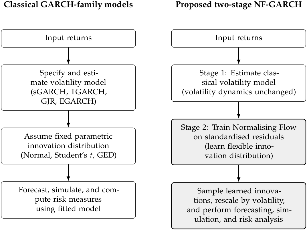
The method operates in two stages. First, standard GARCH models are fitted and standardised residuals are extracted. Second, a normalising flow is trained on these residuals, and flow samples subsequently drive the original GARCH recursion. This preserves the traditional volatility structure and permits modular estimation. The flow’s shape is state-invariant: it scales with ${\sigma }_t$ but does not depend on it. End-to-end designs that jointly optimise flow and GARCH parameters represent a natural extension; we deliberately avoid joint estimation here to maintain interpretability and parameter identifiability, leaving this as a direction for future work.

The remainder of this paper is structured as follows. Section 2 presents the background to volatility modelling, normalising flows, and our two-stage hybrid approach. Section 3 describes the experiment setup. Section 4 presents the results and discussion, and Section 5 concludes.

2. Background

2.1. Volatility Modelling

The foundation of standard Autoregressive Moving Average (ARMA) analysis relies on the assumption that the mean and unconditional variance of the time series remain constant over time, implying stationarity (Box and Jenkins 1976; Pankratz 1991). Techniques such as plotting the Autocorrelation Function (ACF) and Partial Autocorrelation Function (PACF), alongside tests like the Augmented Dickey–Fuller (ADF) test, are employed to ascertain stationarity. For non-stationary time series, transformations are applied to achieve stationarity, as detailed by Pankratz (1991).

In addressing the challenge of high volatility in forecasting financial time series, recent developments have led to the adoption of models like Generalised Autoregressive Conditional Heteroskedasticity (GARCH) models. In GARCH processes, volatility (i.e., the variance of disturbances) is explicitly modelled. Tests for stationarity and other diagnostics closely parallel those used in ARMA analysis. Asymmetric extensions such as EGARCH (Nelson 1991), TGARCH (Zakoian 1994), and GJR-GARCH (Glosten et al. 1993) allow negative shocks to affect volatility differently from positive ones, capturing the leverage effect documented in equity and FX returns (Black 1976; Christie 1982; Cont 2001).

R. F. Engle (1982) showed that the serial correlation in squared returns, or conditional heteroskedasticity, can be modelled using an autoregressive conditional heteroskedasticity (ARCH) model of the following form:

$$Y_t={\mathbb{E}}_{t-1}\left[Y_t\right]+{ϵ}_t$$

(1)

$${ϵ}_t={\sigma }_t{z}_t$$

(2)

$${\sigma }_t^2=a_0+a_1{ϵ}_{t-1}^2+a_2{ϵ}_{t-2}^2+\cdots +a_q{ϵ}_{t-q}^2$$

(3)

where ${\mathbb{E}}_{t-1}[·]$ represents the conditional expectation on all information that is available at time $t-1$ and ${ϵ}_t$ is modelled as the product of a standardised shock $z_t$ and time-varying volatility ${\sigma }_t$ such that $z_t$ is a sequence of independent and identically distributed (“iid”) random variables with mean zero and unit variance. In the ARCH model, $z_t$ is assumed to be independent and identically distributed with a standard normal distribution. The restrictions $a_0>0$ and $a_i>=0$ $i=1,\dots ,q$ are required for ${\sigma }_t^2>0$.

An important extension of the ARCH model proposed by Bollerslev (1986) replaces the AR (p) representation with an ARMA (p,q) formulation:

$${\sigma }_t^2=a_0+\sum _{j=1}^p{b}_j{\sigma }_{t-j}^2+\sum _{i=1}^q{a}_i{ϵ}_{t-i}^2,$$

(4)

where the coefficients $a_i$ $(i=0,\dots ,q)$ and $b_j$ $(j=1,\dots ,p)$ are all assumed to be positive to ensure that the conditional variance ${\sigma }_t^2$ is always positive. The model in Section 2.4 together with Section 2.1 and Section 2.2 is known as the generalised ARCH or GARCH (p,q) model. When $p=0$, the GARCH model reduces to the ARCH model.

2.2. Normalising Flows

Normalising flows represent a robust framework for constructing intricate probability distributions by applying a series of invertible transformations (Mongwe et al. 2025a; Rezende and Mohamed 2015). The initial probability density undergoes a sequence of mappings by systematically employing the change of variables formula, yielding a tractable complex distribution. The term normalising flow aptly describes this process, as the density effectively “flows” through the sequence of transformations, culminating in a normalised probability distribution (Rezende and Mohamed 2015).

Based on the initial framework developed by Rezende and Mohamed (2015), we consider a finite sequence of transformations where each mapping is invertible and smooth. If we let f denote such a mapping with its corresponding inverse $f^{-1}$, then for a random variable $\mathbf{X}$ with an initial density $p_{\mathbf{X}}\left(\mathbf{x}\right)$, the transformed random variable $\mathbf{Y}=f\left(\mathbf{X}\right)$ follows a density

$$p_{\mathbf{Y}}\left(\mathbf{y}\right)=p_{\mathbf{X}}\left(f^{-1}\left(\mathbf{y}\right)\right)\left|det{\displaystyle \frac{\partial f^{-1}\left(\mathbf{y}\right)}{\partial \mathbf{y}}}\right|$$

(5)

This relationship is derived by invoking the inverse function theorem, which governs the behaviour of Jacobians for invertible functions. By composing multiple such mappings, one can generate arbitrarily complex densities. Specifically, if a random variable $\mathbf{X}$ with density $p_{\mathbf{X}}\left(\mathbf{x}\right)$ is subjected to a sequence of K transformations $f_1,f_2,\dots ,f_K$, the resulting density of the final variable ${\mathbf{Z}}_K=f_K\circ \cdots \circ f_1\left(\mathbf{X}\right)$ can be written in terms of the base variable and the Jacobians of the forward maps $p_{{\mathbf{Z}}_K}\left({\mathbf{z}}_K\right)=p_{\mathbf{X}}\left({\mathbf{x}}_0\right){\prod }_{k=1}^K{\left|det{J}_{f_k}\left({\mathbf{z}}_{k-1}\right)\right|}^{-1}$, where ${\mathbf{z}}_0={\mathbf{x}}_0$ and $J_{f_k}$ denotes the Jacobian of $f_k$. Equivalently, in inverse form,

$$p_{{\mathbf{Z}}_K}\left({\mathbf{z}}_K\right)=p_{\mathbf{X}}\left(\mathbf{x}\right)\prod _{k=1}^K\left|det{\displaystyle \frac{\partial f_k^{-1}\left({\mathbf{z}}_k\right)}{\partial {\mathbf{z}}_k}}\right|$$

(6)

As suggested by Kobyzev et al. (2020), the trajectory traced by the sequence of transformed random variables ${\mathbf{Z}}_k$, starting from the initial distribution $p_{\mathbf{X}}\left(\mathbf{x}\right)$, constitutes the flow. In contrast, the sequence of intermediate densities $p_{{\mathbf{Z}}_k}\left({\mathbf{z}}_k\right)$ defines the Normalising Flow.

2.3. Normalising Flows in GARCH Residuals (NF-GARCH)

Traditional GARCH-type models, including sGARCH, EGARCH, and TGARCH, often assume that the residuals $z_t$ follow a known parametric distribution such as Gaussian, Student’s t, or Generalised Error Distribution. However, empirical studies have shown that these fixed-distribution assumptions are often too restrictive to capture the true nature of financial return innovations, which can be skewed, heavy-tailed, or even multi-modal. The choice of innovation distribution is critical for tail-sensitive risk measures such as Value-at-Risk and Expected Shortfall (Bauwens et al. 2006; Hansen 1994).

To address this, we replace the assumption $z_t\sim \mathcal{N}(0,1)$ with the following:

$$z_t=f\left(u_t\right),u_t\sim \mathcal{N}(0,I_d)$$

where $f:{\mathbb{R}}^d\to {\mathbb{R}}^d$ is a sequence of invertible, differentiable transformations—i.e., a normalising flow. This transforms a simple base distribution (such as standard normal) into a rich, learned distribution for residuals $z_t$, thereby enabling greater flexibility in capturing empirical data characteristics. While alternative heavy-tailed base distributions such as Student’s t could be considered for the base distribution, we adopt a standard normal base for tractability and comparability, with tail flexibility introduced through the learned flow transformations.

Given a base density $p_U\left(u\right)$ and an invertible transformation $z=f\left(u\right)$, the transformed density of z is given by the change-of-variables formula:

$$p_Z\left(z\right)=p_U\left(f^{-1}\left(z\right)\right)\left|det\left({\displaystyle \frac{\partial f^{-1}\left(z\right)}{\partial z}}\right)\right|$$

or, equivalently,

$$\log p_Z\left(z\right)=\log p_U\left(u\right)-\sum _{i=1}^K\log \left|det\left({\displaystyle \frac{\partial f_i}{\partial h_{i-1}}}\right)\right|$$

where $f=f_K\circ \cdots \circ f_1$, and $h_i=f_i\left(h_{i-1}\right)$ with $h_0=u$. Popular choices for flows include RealNVP (Dinh et al. 2016), Masked Autoregressive Flows (MAF) (Papamakarios et al. 2017), and Neural Spline Flows (Durkan et al. 2019). Although these flows are commonly constructed using a standard normal base distribution, heavier-tailed behaviour can be accommodated through sufficiently expressive transformations, and alternative base distributions could be considered as extensions.

2.4. NF-GARCH Model Structure

The NF-GARCH model can be represented as follows:

$$\begin{array}{cc}\hfill Y_t& ={\mu }_t+{ϵ}_t\hfill \end{array}$$

(7)

$$\begin{array}{cc}\hfill {ϵ}_t& =z_t{\sigma }_t,z_t=f\left(u_t\right),u_t\sim \mathcal{N}(0,1)\hfill \end{array}$$

(8)

$$\begin{array}{cc}\hfill {\sigma }_t^2& =\omega +\sum _{i=1}^q{\alpha }_i{ϵ}_{t-i}^2+\sum _{j=1}^p{\beta }_j{\sigma }_{t-j}^2\hfill \end{array}$$

(9)

Empirical specification (notation). The system above uses general orders $(p,q)$ for exposition. In all experiments we estimate constant-mean log-return models, $r_t=\mu +{ϵ}_t$, where the scalar $\mu$ is estimated by maximum likelihood jointly with volatility parameters (no ARMA dynamics in the mean). The conditional variance follows each variant’s GARCH(1,1)-type recursion as implemented in our custom R engine: sGARCH updates ${\sigma }_t^2$ via the standard GARCH(1,1) recursion; TGARCH models the conditional scale ${\sigma }_t$ directly per Zakoian (1994); GJR-GARCH adds an asymmetric leverage term $I_{t-1}{ϵ}_{t-1}^2$ to the variance recursion; and eGARCH models $\log {\sigma }_t^2$ with asymmetric terms per Nelson (1991). Standardised residuals passed to the flow are ${\widehat{z}}_t=(r_t-\widehat{\mu })/{\widehat{\sigma }}_t$ using in-sample fitted values only. In tables, the label norm denotes Gaussian innovations; sstd denotes skewed Student’s t innovations in the parameterisation of Fernández and Steel (1998) and Hansen (1994).

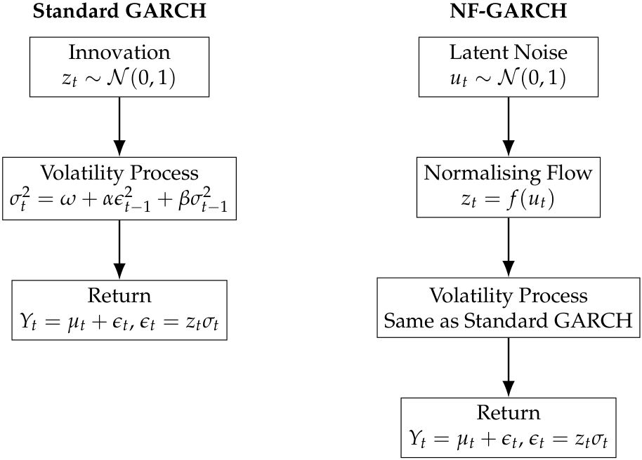
Figure 1 highlights the modular nature of the NF-GARCH framework: the normalising flow modifies only the innovation distribution, while the volatility recursion remains structurally identical to classical GARCH models.

In principle, the parameters of both the volatility recursion and the flow can be estimated by maximising the likelihood implied by the GARCH recursion combined with the flow-induced residual density $p_Z\left(z\right)$. This framework allows the volatility process to follow the standard GARCH formulation while modelling the innovation distribution as a flexible, non-Gaussian transformation of a simple base distribution.

2.5. Benefits of NF-GARCH

The integration of normalising flows into GARCH models enables the capture of skewness and heavy tails through flexible invertible transformations, without imposing restrictive parametric constraints on the innovation law, while preserving exact likelihoods for estimation. The resulting residual distribution facilitates realistic simulation and stress testing. Notably, the volatility process remains interpretable because the variance recursion is unchanged, even as the flexibility of the residuals increases. This hybrid framework isolates the contribution of distributional flexibility without altering the volatility structure, thereby allowing the assessment of whether a more expressive innovation law enhances forecasting accuracy, scenario generation, and the replication of stylized facts.

This hybrid approach allows us to assess whether distributional flexibility alone (i.e., with no change to the volatility structure) can significantly improve forecasting, scenario simulation, and stylized fact replication.

2.6. Theoretical Considerations

Normalising flows offer a flexible and tractable approach for modelling innovation distributions; however, their integration with GARCH-family volatility recursions introduces several important theoretical considerations.

2.6.1. Identifiability

Within the NF-GARCH framework, the conditional variance ${\sigma }_t^2$ is determined by the GARCH recursion, while the flow $f_{\theta }(·)$ transforms latent noise $u_t$ into residuals $z_t$. There is a potential for a confounding effect between the volatility parameters and the transformations learned by the flow as both components influence the scale and shape of the simulated return given that

$$r_t={\mu }_t+{ϵ}_t,{ϵ}_t={\sigma }_t{z}_t,z_t=f_{\theta }\left(u_t\right),$$

If the flow is excessively flexible, it may absorb variation that would otherwise be attributed to the volatility recursion, leading to partial non-identifiability between scale parameters in ${\sigma }_t$ and in $f_{\theta }$. Formally, writing $r_t={\sigma }_t{f}_{\theta }\left(u_t\right)$, if $f_{\theta }$ includes an arbitrary scaling component then ${\sigma }_t{f}_{\theta }\left(u_t\right)=\left({\sigma }_{t}c\right){\tilde{f}}_{\theta }\left(u_t\right)$ for some constant c, so scale can be reallocated between the volatility recursion and the flow, implying partial scale non-identifiability. This is an inherent limitation of combining highly expressive innovation laws with parametric volatility models, which becomes even more important when one wants to jointly calibrate the parameters of the underlying GARCH model with that of the Normalising Flow.

2.6.2. Overfitting in Expressive Flows

As with any deep learning model, normalising flows with numerous layers or high-capacity coupling networks are susceptible to overfitting the empirical residual distribution, particularly when applied to short financial time series (Mongwe et al. 2025b). Since flows are trained by maximising likelihood, they may capture spurious high-frequency structure or noise instead of the underlying innovation law. In volatility modelling, such overfitting can distort tail behaviour, degrade out-of-sample forecast performance, and yield misleading risk measures. Therefore, controlling model capacity, such as by limiting flow depth or width and employing regularisation techniques, is essential in NF-GARCH design (Mongwe et al. 2025b).

2.6.3. Likelihood Regularisation and Numerical Stability

Flow-based likelihoods require computation of the Jacobian log-determinant,

$$\log p_Z\left(z\right)=\log p_U\left(f_{\theta }^{-1}\left(z\right)\right)+\log \left|det{J}_{f_{\theta }^{-1}}\left(z\right)\right|,$$

which can become numerically unstable if the transformations are too deep or poorly conditioned. Large positive or negative Jacobian terms can lead to exploding or vanishing log-densities and hinder convergence in optimisation (Papamakarios et al. 2021). Practical implementations often mitigate these issues through weight decay, spectral constraints, or penalties on extreme Jacobian values to keep the learned density well-behaved (Papamakarios et al. 2021).

2.6.4. Sensitivity to Flow Depth and Architecture

While deeper flows are theoretically more expressive, Papamakarios et al. (2021) confirmed that they also increase computational cost and may interact unfavourably with long-memory volatility dynamics. In practice, shallow or moderately deep flows often provide sufficient flexibility to capture skewness and heavy tails in the residuals, whereas very deep architectures yield diminishing returns and intensify identifiability and stability concerns (Liu and Regier 2020). Consequently, parsimonious flow architectures are generally preferable when integrating flows into GARCH-type models.

2.6.5. Implications for NF-GARCH

These considerations indicate that NF-GARCH models function as semi-parametric volatility models, with their advantages contingent upon achieving a careful balance between flexibility and control. The GARCH recursion maintains its interpretability, whereas the innovation law becomes a learned component that requires regularisation to prevent overfitting and instability. Thus, a theoretically robust NF-GARCH specification necessitates careful attention to both the volatility structure and the capacity and regularisation of the flow.

2.7. Two-Stage NF Innovations vs. End-to-End Flow-After-Scaling

Two-stage. In this framework, the normalising flow is trained after the standard GARCH estimation stage, rather than being embedded directly into the volatility recursion. This modular approach separates the estimation of conditional volatility dynamics from the learning of the innovation distribution, allowing for a clearer interpretation of each component. Specifically, we model the following:

$$r_t={\mu }_t+{ϵ}_t,{ϵ}_t={\sigma }_t{z}_t^{\prime },z_t^{\prime }\sim p_{\mathrm{NF}},$$

with ${\sigma }_t^2$ following the usual GARCH recursion and $p_{\mathrm{NF}}$ learned from the standardised residuals ${\widehat{z}}_t=(r_t-{\widehat{\mu }}_t)/{\widehat{\sigma }}_t$. Estimation is modular: first fit a GARCH model under a standard innovation assumption (Gaussian or skew-t) to obtain ${\widehat{\sigma }}_t$, then train a flow on $\left\{{\widehat{z}}_t\right\}$. Forecasts and simulations draw $z_t^{\prime }\sim p_{\mathrm{NF}}$ and propagate through the same recursion.

Joint (end-to-end) training. An alternative modelling strategy would estimate the GARCH volatility parameters and the normalising flow jointly within a single likelihood function, which is a flow-after-scaling or end-to-end calibration approach. In such a framework, the innovations are modelled as

$$z_t=f_{\varphi }\left(u_t\right),u_t\sim \mathcal{N}(0,1),{ϵ}_t={\sigma }_t\left(\theta \right)z_t,$$

where both $(\theta ,\varphi )$ are estimated simultaneously by maximising the joint log-likelihood ${\sum }_t{\mathit{\ell }}_t(\theta ,\varphi )$. This allows the flow to adapt to the evolving volatility state and enables fully data-driven conditional innovation laws, but it introduces a highly non-convex objective and greater computational cost.

While theoretically appealing, this approach introduces substantial practical and conceptual challenges. Joint calibration entangles the scale effects of the volatility recursion with the shape flexibility of the flow, leading to partial identifiability between ${\sigma }_t\left(\theta \right)$ and $f_{\varphi }(·)$. As a result, improvements in likelihood or forecasting accuracy cannot be uniquely attributed to enhanced volatility dynamics or improved innovation modelling. In addition, the resulting optimisation problem is highly non-convex and numerically unstable, particularly for asymmetric volatility specifications such as EGARCH.

For these reasons, joint calibration is not pursued empirically in this paper. Joint estimation was not pursued due to numerical instability and the need to isolate the marginal contribution of innovation modelling. Instead, a two-stage design is adopted to deliberately isolate the contribution of flexible innovation distributions while preserving the classical GARCH volatility structure. Nevertheless, joint flow–GARCH estimation remains an important and promising direction for future research, particularly in settings where conditional density calibration is prioritised over interpretability.

2.8. Relationship to Classical GARCH

The proposed NF-GARCH framework strictly generalises the classical GARCH model. In particular, standard GARCH with Gaussian innovations is recovered as a special case when the normalising flow reduces to the identity transformation

$$f\left(u\right)=u,$$

so that

$$z_t=f\left(u_t\right)=u_t\sim \mathcal{N}(0,1).$$

Under this restriction, the NF-GARCH model collapses exactly to the conventional GARCH specification with Gaussian residuals. Hence, classical GARCH models lie on the boundary of the NF-GARCH model class.

It is important to note, however, that this nesting is conceptual rather than operational: in the two-stage framework adopted in this paper, the flow is not jointly estimated with the volatility recursion, and the identity mapping is not imposed during training. As such, standard GARCH is not recovered through estimation but represents a limiting case within the broader NF-GARCH modelling space. A comparison of innovation structures in standard GARCH and in the NF-GARCH framework are shown in Figure 2.

3. Experiment Setup

3.1. Data Description

Our empirical analysis utilises a dataset comprising 13 daily financial time series, spanning the period from 31 August 2005, to 31 August 2024. The sample encompasses six foreign exchange (FX) pairs (USD/ZAR, GBP/USD, EUR/USD, GBP/CNY, GBP/ZAR, and EUR/ZAR) alongside seven highly capitalized equities (X, NVDA, MSFT, PG, CAT, WMT, and AMZN). FX data were obtained from the South African Reserve Bank and OANDA, while equity price data were retrieved from Yahoo Finance. All series were systematically aligned to exclude non-trading days. Because this sample predominantly represents highly liquid, major asset classes and widely traded emerging market currencies, we caution that the empirical findings may not directly generalise to alternative asset classes such as commodities, fixed-income instruments, or illiquid frontier markets.

Asset selection rationale. Assets were selected to span two liquid classes—major and ZAR-denominated FX pairs and large-cap multi-sector equities—that are well known to exhibit GARCH-type conditional heteroskedasticity and heavy-tailed innovations. Including ZAR pairs (USD/ZAR, GBP/ZAR, EUR/ZAR) introduces emerging-market currency dynamics alongside G10 benchmarks (GBP/USD, EUR/USD). The equities cover technology (NVDA, MSFT), consumer staples (PG, WMT), industrials (CAT, X), and e-commerce (AMZN), providing sector diversity. This composition allows comparison across asset classes while remaining computationally feasible; extension to commodities, fixed income, and frontier markets is noted as a direction for future work.

Returns and cleaning. We work with log returns $r_t=\log (P_t/P_{t-1})$ computed on business days. Prices are aligned to each asset’s trading calendar; non-trading days and missing values are dropped. Extreme single-day spikes are retained without winsorisation so that tail behaviour is preserved for flow training and VaR analysis. A minimum of 520 valid observations is required per asset (500 training + 20 test); assets or windows that fail to reach this threshold are excluded. Return series are treated as weakly stationary following standard practice, with formal residual diagnostics after GARCH filtering reported in Section 3.5.

3.2. Data Preparation and Performance Evaluation

To preserve the inherent temporal dynamics of the sample, we partition the dataset chronologically, allocating 65% to the training set and 35% to the test set. Robustness is further established through a rolling-window time-series cross-validation framework. Within this framework, each cross-validation fold comprises a training window of 500 observations followed immediately by a 20-observation test window, advancing in discrete, non-overlapping 500-observation increments. To manage computational feasibility while ensuring representative temporal coverage, we subsampled up to three evenly spaced folds per asset–model pair. Consequently, these validation windows strategically capture the early, mid, and late evaluation periods across all 13 analysed assets and their respective models.

To strictly preclude look-ahead bias, we enforce strict chronological ordering: each training window spans the interval from $t_{\mathrm{start}}$ to $t_{\mathrm{start}}+499$, with the subsequent 20 observations designated for out-of-sample testing. Consequently, a minimum threshold of 520 valid observations is required for an asset to be included in the sample. Furthermore, the final analysis is restricted exclusively to models that successfully achieve convergence. To evaluate predictive accuracy and model fit, we calculate the mean squared error (MSE), Mean Absolute Error (MAE), Akaike Information Criterion (AIC), and Bayesian Information Criterion (BIC) independently for each window before computing their overall averages. This localized evaluation framework captures performance heterogeneity across diverse market regimes and mitigates reliance on any single temporal period.

3.3. Model Development and Implementation

The GARCH models are implemented in R (version 4.4.1; R Core Team, Vienna, Austria) using a custom estimation engine. This gives complete control over parameterisation and diagnostics. We fit four variants per asset: standard GARCH (normal and Student-t innovations), Exponential GARCH (asymmetric effects), Glosten–Jagannathan–Runkle GARCH (leverage terms), and Threshold GARCH (regime-dependent responses). Maximum likelihood estimation uses R’s optim function. We evaluate models using AIC, BIC, MSE, MAE, and residual diagnostics (Ljung–Box and ARCH–LM).

For the normalising flow, we extract standardised residuals from each fitted GARCH model and train an independent flow model using the nflows (version 0.14.0) library in Python (version 3.14). The main experiments use a Masked Autoregressive Flow (MAF); an architecturally distinct Real NVP model is trained under identical hyperparameters for the multi-seed robustness comparison. Architecture details and a side-by-side specification appear in

Table 1. Normalising flow architecture specifications ^†.

Component	MAF (Main)	RealNVP (Robustness)
Architecture
Transform Type	Masked Autoregressive Flow	Real Non-Volume Preserving
Coupling	Autoregressive affine; masked connections	Non-autoregressive affine coupling
Masking	Autoregressive ordering	Input split into two halves
Residual Blocks	—	2 per coupling layer
Shared hyperparameters
Base Distribution	Standard Normal $\mathcal{N}(0,1)$
Layers	4
Hidden Units	64 per layer
Activation	ReLU
Optimizer	Adam
Learning Rate	${10}^{-3}$
Batch Size	512
Max. Epochs	75
Early Stopping	Patience = 15 epochs (validation log-likelihood)
Validation Split	20% of training data
Weight Decay	${10}^{-5}$

^† Note: Both architectures use the nflows Python library (MAF: MaskedAffineAutoregressiveTransform; RealNVP: RealNVP class). MAF is used for all main experiments; RealNVP is applied with identical shared hyperparameters for the multi-seed robustness comparison (Section 4.9). RealNVP replaces autoregressive masking with non-autoregressive affine coupling layers, preserving exact invertibility and tractable log-determinant computation. —: not applicable (residual blocks apply to RealNVP coupling layers only; MAF does not use them).

.

Rationale for MAF. Among flow architectures, Masked Autoregressive Flows (Papamakarios et al. 2017) are a standard choice for low-dimensional univariate density estimation: they yield analytically tractable Jacobians, numerically stable maximum-likelihood training on residuals, and an autoregressive factorisation that naturally matches the univariate innovation setting. Real NVP (Dinh et al. 2016) and Neural Spline Flows (Durkan et al. 2019) are architecturally distinct alternatives mentioned in the paper; we adopt MAF for the main experiments after a constrained sensitivity check over depth, width, learning rate, and batch size (Section 3.4), prioritising validation likelihood and numerical stability. We extend the empirical comparison to Real NVP (Dinh et al. 2016) on the same evaluation protocol and report multi-seed stability results across seeds 123, 456, and 789 for both architectures in Section 4.9.

MAF transforms the base distribution through a series of invertible autoregressive layers (Papamakarios et al. 2017). Each layer applies an affine transformation $y_i=x_i·exp\left(s_i\left({\mathbf{x}}_{<i}\right)\right)+t_i\left({\mathbf{x}}_{<i}\right)$, where the scale $s_i$ and shift $t_i$ are conditioned only on preceding dimensions, ensuring strict invertibility and analytically tractable Jacobians. Post-training, NF-GARCH models are synthesised for simulation and forecasting by integrating the flow-generated innovations into the original GARCH recursion. While this study is confined to a univariate framework, extending the methodology to capture joint market dynamics via multivariate models (e.g., Multivariate GARCH (Bollerslev 1990), BEKK-MGARCH (Engle and Kroner 1995), or Dynamic Conditional Correlation (R. Engle 2002)) remains a compelling direction for future work.

Note that the described two-stage procedure prevents data leakage as follows:

• Data splitting: Split chronologically—65% training, 35% test.
• Stage 1—GARCH estimation:
  • Estimate GARCH parameters on training set only: ${\mathit{\theta }}_{\mathrm{GARCH}}^{\ast }=arg{max}_{\mathit{\theta }}{\sum }_{t\in \mathrm{train}}{\mathit{\ell }}_{\mathrm{GARCH}}(r_t;\mathit{\theta })$;
  • Extract standardised residuals:${\widehat{z}}_t=(r_t-{\widehat{\mu }}_t)/{\widehat{\sigma }}_t$ for $t\in \mathrm{train}$, where ${\widehat{\sigma }}_t$ uses ${\mathit{\theta }}_{\mathrm{GARCH}}^{\ast }$.
• Stage 2—NF training:
  • Train flow on training-set residuals only: ${\mathit{\varphi }}^{\ast }=arg{max}_{\mathit{\varphi }}{\sum }_{t\in \mathrm{train}}\log p_f({\widehat{z}}_t;\mathit{\varphi })$;
  • Test-set information never enters NF training.
• Stage 3—NF-GARCH simulation and forecasting:
  • Sample residuals from trained NF: ${\tilde{z}}_t\sim p_f(·;{\mathit{\varphi }}^{\ast })$.;
  • Forecast on test set: ${\tilde{r}}_t={\widehat{\mu }}_t+{\tilde{z}}_t{\widehat{\sigma }}_t$ for $t\in \mathrm{test}$;
  • Evaluate using test-set returns only.

Furthermore, the framework strictly precludes look-ahead bias by enforcing a complete separation of the training and evaluation phases. Specifically, the GARCH parameters and their corresponding residuals are estimated exclusively on the training sample. The normalising flow is subsequently trained solely on these in-sample residuals, reserving the test set strictly for out-of-sample evaluation. This sequential methodology inherently assumes residual stationarity across both the training and test periods—an assumption we rigorously validate using Augmented Dickey–Fuller (ADF), KPSS, Ljung-Box, and ARCH-LM tests (see Section 3.5).

3.4. Hyperparameter Selection and Model Capacity Control

The implementation of normalising flows necessitates the specification of various architectural and optimisation hyperparameters. We followed a two-phase selection protocol. First, the final 20% of each training window was withheld as a held-out validation set before any hyperparameter search began, ensuring no overlap with the test period. Second, we evaluated candidate configurations over network depth (3–6 layers), width (32–128 hidden units), learning rates ($[5\times {10}^{-4},2\times {10}^{-3}]$), and batch sizes (256–1024); the configuration achieving the highest mean validation log-likelihood across assets and GARCH specifications was retained. The finalised Masked Autoregressive Flow (MAF) architecture comprises four layers with 64 hidden units each, using a batch size of 512. The network is optimised via the Adam algorithm with a learning rate of ${10}^{-3}$, incorporating an early stopping mechanism triggered after 15 epochs without improvement in validation log-likelihood. The same hyperparameters were applied without re-tuning to the RealNVP robustness comparison in Section 4.9, providing a controlled architectural comparison.

Notably, expanding the network’s capacity—either in depth or width—yielded negligible in-sample improvements while inducing erratic fluctuations in the Jacobian log-determinants and pronounced overfitting, particularly on shorter time series. To mitigate these instabilities, we explicitly restricted the architectural depth and applied $L_2$ regularisation with a weight decay parameter of ${10}^{-5}$.

3.5. Residual Stationarity Diagnostics

The two-stage approach assumes standardised residuals

$${\widehat{z}}_t={\displaystyle \frac{r_t-{\widehat{\mu }}_t}{{\widehat{\sigma }}_t}}$$

are weakly stationary after GARCH filtering, suitable for density estimation. We test this for each asset–model pair using: Augmented Dickey–Fuller (unit root), KPSS (stationarity), autocorrelation functions for ${\widehat{z}}_t$ and ${\widehat{z}}_t^2$, Ljung–Box Q-statistics for raw and squared residuals, and ARCH-LM tests for remaining heteroskedasticity.

ADF tests reject unit roots for all models and assets. KPSS indicates stationarity for most series. GARCH filtering largely removes serial dependence in ${\widehat{z}}_t$; some squared residuals show minor remaining dependence. ARCH-LM shows substantial—but not complete—heteroskedasticity reduction.

Table 2. Summary of residual stationarity diagnostics.

Test	Mean p-Value	Pass Rate (%)	Interpretation
ADF (unit root)	0.012	94.4	Most residuals reject non-stationarity
KPSS (stationarity)	0.087	88.9	Most residuals fail to reject stationarity
Ljung-Box (${\widehat{z}}_t$)	0.156	83.3	Most residuals show no serial correlation
Ljung-Box (${\widehat{z}}_t^2$)	0.089	77.8	Some squared residuals retain dependence
ARCH-LM	0.124	72.2	Most residuals show reduced heteroskedasticity

Note: Pass rates indicate the percentage of model–asset combinations where tests support the null hypothesis (for ADF, KPSS, Ljung-Box) or fail to reject homoskedasticity (for ARCH-LM). Lower p-values for ADF and KPSS, and higher p-values for Ljung-Box and ARCH-LM, indicate better residual properties. Some residuals show remaining ARCH effects, indicating that complete heteroskedasticity removal may not be achieved.

summarises the diagnostics. Most series pass stationarity tests (ADF, KPSS) with mean p-values strongly against non-stationarity. Ljung-Box shows most residuals are approximately uncorrelated; some squared residuals retain dependence. ARCH-LM indicates substantially reduced heteroskedasticity, though some series keep mild ARCH effects. These support the weak stationarity assumption for flow-based density estimation, while acknowledging that complete heteroskedasticity removal is not universal.

3.6. Theoretical Properties of Two-Stage Estimation

Two-stage estimation needs theoretical justification. Under regularity conditions (Newey and McFadden 1994), consistency requires: (1) Stage 1 (GARCH) is consistent, (2) Stage 2 (NF) depends on Stage 1 only through residuals, and (3) residual distribution is stationary across training and test periods.

Two-stage is less efficient than joint maximum likelihood as it ignores cross-equation information between GARCH and flow parameters. Practical advantages: separate optimisation (computationally tractable), numerical stability (avoids high-dimensional joint optimisation), and flexibility (different methods per stage). Efficiency loss is typically small when residuals are approximately stationary, which we validate via diagnostics; formal efficiency comparison with joint one-step extremum estimators is left for future work.

Validity requires: (1) GARCH and NF parameters are separately identifiable, (2) residual distribution is stationary (ADF/KPSS), and (3) no functional dependence between GARCH and NF parameter spaces. Identifiability holds because GARCH controls volatility dynamics while NF controls residual shape, which are distinct model aspects.

3.7. Conditional vs. Unconditional Innovation Modelling

Our two-stage design models the standardised residuals using a time-invariant unconditional distribution, acknowledging that financial innovations may occasionally exhibit mild conditional heterogeneity during periods of acute market stress. In this framework, all temporal dynamics in volatility are captured exclusively by the GARCH recursion via the conditional standard deviation, ${\sigma }_t$. Concurrently, the normalising flow specifies a highly flexible, yet time-invariant, distribution for the innovations. This architectural choice structurally mirrors classical GARCH specifications, wherein innovations are assumed to be independent and identically distributed (i.i.d.) according to a fixed parametric law (e.g., Gaussian, Student’s t, or Generalised Error Distribution). The NF-GARCH model retains this foundational structure but substitutes the rigid parametric density with a data-driven, highly parameterised distribution learned via the flow.

To validate the assumption of a time-invariant innovation distribution, we conducted a battery of robustness checks, including rolling-variance metrics, structural break tests, and subsample distributional comparisons. The results confirm that while the underlying return series exhibit the expected time-varying conditional variance, the standardised residual distributions display no substantial structural breaks and demonstrate limited instability, thereby empirically supporting our time-invariant modelling approach. Although fully conditional or state-dependent normalising flows could theoretically capture more complex distributional dynamics, such extensions introduce significant identifiability and optimisation challenges, rendering them a subject for future research.

3.8. Model Evaluation and Predictions

To rigorously assess the out-of-sample predictive accuracy and distributional fidelity of the final models, we implement a comprehensive dual-evaluation framework on a held-out test set. The first phase evaluates the quality of the synthetic residuals generated by the normalising flows. We employ a robust suite of distributional diagnostics, comprising the (1) Kolmogorov–Smirnov statistic, (2) Wasserstein-1 distance, (3) the Hill estimator for tail indices, (4) skewness, and (5) kurtosis to verify that the flow-injected innovations successfully replicate the key empirical properties of the underlying financial data.

The second phase quantifies explicit forecasting performance utilising the previously outlined 65/35 chronological split and rolling-window time-series cross-validation. Model efficacy is measured via the mean squared error (MSE), Mean Absolute Error (MAE), out-of-sample log-likelihood, AIC, and BIC. To determine the statistical significance of performance differentials across matched model–asset–window evaluations, we apply the non-parametric Wilcoxon signed-rank test (Demšar 2006). Furthermore, forecast win-rates are computed to provide an interpretable summary of relative model superiority, aligning with established best practices in volatility forecasting (Amisano and Giacomini 2007; Ziel 2016). Finally, through a combination of visual diagnostics and these formal distributional metrics, we systematically verify the replication of stylized financial facts. This confirms that the performance gains observed in the NF-augmented models represent robust, structural improvements rather than transient initialisation artifacts.

3.9. Stress Testing Framework and Scenario Analysis

To rigorously evaluate the predictive stability of the proposed framework under extreme market conditions, we implement a comprehensive stress-testing protocol encompassing historical crisis scenarios. The historical analysis examines two periods of acute market dislocation: the Global Financial Crisis (1 September 2008–31 March 2009) and the COVID-19 market crash (1 February 2020–30 April 2020). To maintain strict out-of-sample integrity, models are calibrated exclusively on pre-crisis data and subsequently evaluated during these defined crisis windows. Forecasting performance across all scenarios is quantified via MSE and MAE. We acknowledge that the scope of this evaluation is limited to two specific historical crises. While incorporating supplementary historical stress periods and formally integrating regime-switching tests would further validate the model’s robustness, such computationally intensive extensions remain vital avenues for future research.

4. Results and Discussion

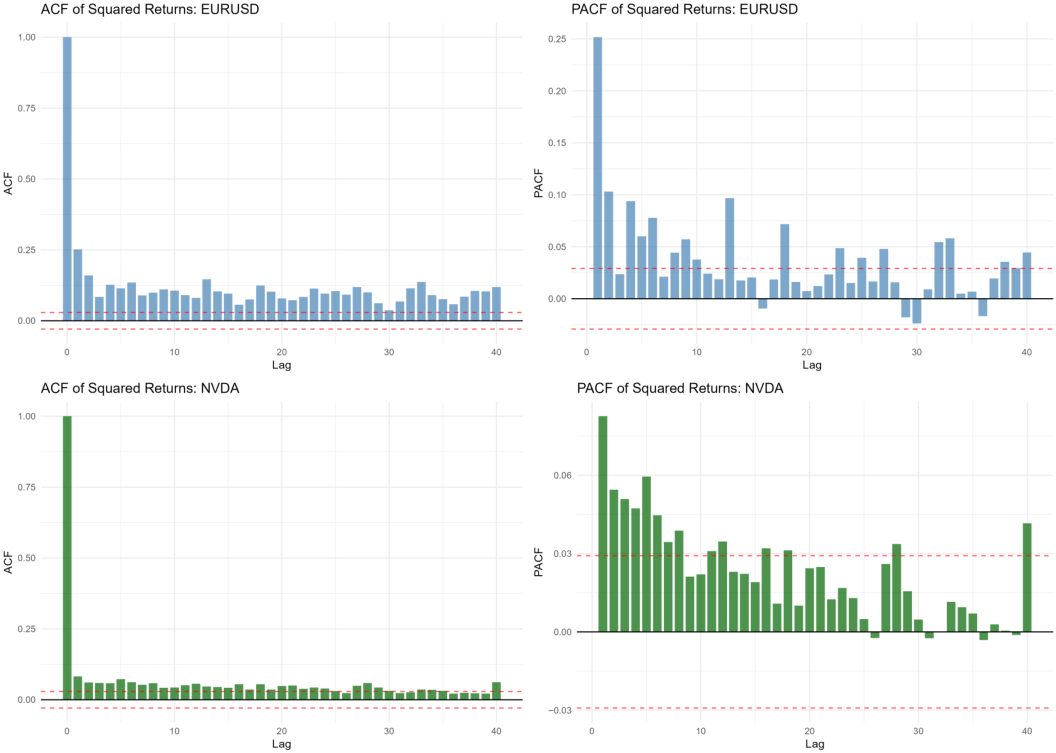
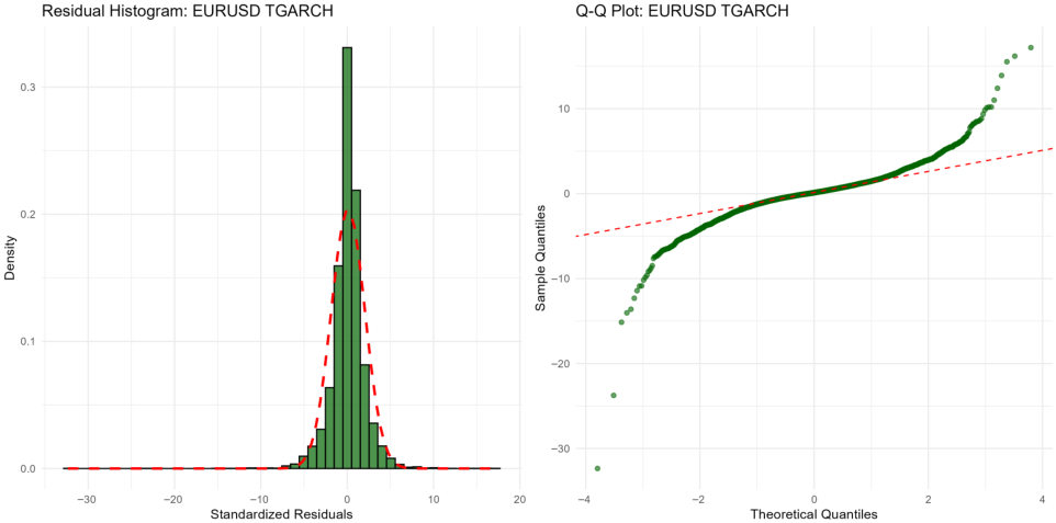
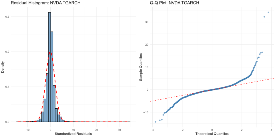
In this section, we present the results of the experiments. Figure 3 shows the autocorrelation and partial autocorrelation functions of the EURUSD (FX) and NVDA (equity) instruments respectively as examples. Figure 4 and Figure 5 show the histograms and Q-Q plots for the same two assets. Table 3 shows the stylized facts by the FX and Equity asset classes. Table 4 displays the baseline GARCH model performance. Table 5 shows the overall performance of standard GARCH compared to NF-GARCH, while Table 6 shows the performance of standard GARCH compared to NF-GARCH by model and distribution. Table 7 shows the Wilcoxon signed-rank test results for standard GARCH compared to NF-GARCH. Table 8 shows the performance of the NF-GARCH model, while Table 9 shows the win rate of NF-GARCH by model and distribution. Table 10, Table 11, Table 12, Table 13 and Table 14 show the distributional realism results of the proposed method.

4.1. Stylized Facts of Return Series

Figure 3 shows autocorrelation and partial autocorrelation functions of squared returns, using the EURUSD and NVDA instruments as examples. Histograms and Q-Q plots (Figure 4 and Figure 5) show deviations from Normality. Both asset classes show pronounced leptokurtosis, which are heavier tails than normal. That is, extreme returns are more likely than Gaussian models predict.

Persistent autocorrelation seen in Figure 3 confirms conditional heteroskedasticity, which is that large shocks tend to follow large shocks. Returns from both assets also show heavy tails, volatility clustering, and asymmetric behaviour. The returns are not normal, and they are not independent over time. Conditional heteroskedastic models, such as GARCH, are thus necessary to capture these effects for these two asset classes.

Table 3 shows key metrics relating to the stylized facts of the two asset classes under consideration. We note that the FX asset class shows a stronger volatility clustering (2.174) than equities (1.817), consistent with a higher frequency and liquidity of FX trading. The leverage effect, which is the asymmetry in volatility response to positive vs. negative shocks, is small but negative for FX (−0.008). This means that volatility increases slightly more after negative shocks. Equities show a marginally positive coefficient (0.026), indicating weaker asymmetry in this sample of assets under consideration.

The FX asset class also shows mild negative skewness (−0.168). Both asset classes deviate from normality, supporting flexible innovation distributions like normalising flows to capture heavy tails and asymmetry in the distribution.

Table 3. Stylized facts by the Equity and FX asset classes (class means of per-asset metrics) ^c.

Asset Class	Volatility Clustering	Leverage Effect	Gain/Loss Asymmetry	Skewness
Equity	1.817	0.026	0.975	0.013
FX	2.174	−0.008	0.987	−0.168

^c Note: Volatility clustering is the sum of the first ten ordinates of the sample ACF vector of squared returns from R’s stats::acf (indexing includes the lag-zero term in that vector). Leverage effect is the mean over $h=1,\dots ,5$ of $\mathrm{corr}\left(1\{r_t<0\},r_{t+h}^2\right)$. Gain/loss asymmetry is $\overline{|r_t|:r_t<0}/\overline{r_t:r_t>0}$ (mean absolute negative return divided by mean positive return). Skewness is moments::skewness when available, otherwise the standardised third moment of $r_t$. Definitions match scripts/evaluation/calculate_stylized_facts.R.

Table 3. Stylized facts by the Equity and FX asset classes (class means of per-asset metrics) ^c.

Asset Class	Volatility Clustering	Leverage Effect	Gain/Loss Asymmetry	Skewness
Equity	1.817	0.026	0.975	0.013
FX	2.174	−0.008	0.987	−0.168

^c Note: Volatility clustering is the sum of the first ten ordinates of the sample ACF vector of squared returns from R’s stats::acf (indexing includes the lag-zero term in that vector). Leverage effect is the mean over $h=1,\dots ,5$ of $\mathrm{corr}\left(1\{r_t<0\},r_{t+h}^2\right)$. Gain/loss asymmetry is $\overline{|r_t|:r_t<0}/\overline{r_t:r_t>0}$ (mean absolute negative return divided by mean positive return). Skewness is moments::skewness when available, otherwise the standardised third moment of $r_t$. Definitions match scripts/evaluation/calculate_stylized_facts.R.

4.2. Baseline GARCH Performance

We estimated classical GARCH models with Gaussian and Student’s t innovations. Table 4 summarises results on the 65/35 chronological split, reporting the mean MSE, MAE, AIC, BIC, and log-likelihood across assets and models.

Table 4. Baseline GARCH model performance using a 65/35 chronological split.

Model	Number of Assets	Mean MSE	Mean MAE	Mean AIC	Mean BIC	Mean LogLik
gjrGARCH	13	0.000355	0.01151	−17,512.32	−17,476.42	8762.16
TGARCH	13	0.000355	0.01149	−16,492.24	−16,456.34	8252.12
sGARCH	13	0.000372	0.01186	−15,337.51	−15,313.58	7672.76
eGARCH	1	0.000553	0.01724	635.79	671.69	−311.89

Table 4. Baseline GARCH model performance using a 65/35 chronological split.

Model	Number of Assets	Mean MSE	Mean MAE	Mean AIC	Mean BIC	Mean LogLik
gjrGARCH	13	0.000355	0.01151	−17,512.32	−17,476.42	8762.16
TGARCH	13	0.000355	0.01149	−16,492.24	−16,456.34	8252.12
sGARCH	13	0.000372	0.01186	−15,337.51	−15,313.58	7672.76
eGARCH	1	0.000553	0.01724	635.79	671.69	−311.89

The baseline results in Table 4 show strong persistence of the variance, which is typical for daily returns, with a slow volatility response to new shocks. TGARCH and GJR-GARCH perform competitively on MSE and MAE. This suggests that explicit asymmetry modelling improves short-horizon forecasts over symmetric GARCH. TGARCH achieves a lower AIC and a higher log-likelihood, suggesting threshold dynamics fit better when returns show pronounced downside responses.

We observe that the eGARCH model underperformed overall. This is due to unstable fits and substantially higher errors. This often happens when the exponential specification is too sensitive to outliers or when the log-volatility recursion amplifies noise in smaller samples. Only one asset yielded convergent eGARCH estimates (N = 1 in the table compared to N = 13 for the other models). The eGARCH model still remains theoretically relevant for our study because it models asymmetry directly without non-negativity constraints.

4.3. EGARCH and TGARCH Convergence

The results in Table 4 show that the standard TGARCH with skewed-t innovations converges for all 13 assets. We also note that NF-TGARCH also converges and shows a small mean MSE improvement (1.2%) as shown in Table 6. NF-EGARCH fails to converge in 12 of 13 assets. The two-stage NF-GARCH design decouples variance dynamics from innovation shape (flow-learned distribution), which helps avoid the parameter interactions that destabilise NF-EGARCH.

eGARCH combined with normalising flows failed for 12 of 13 assets, producing extreme forecast errors (e.g., $4.15\times {10}^{66}$). Two factors explain this: (1) eGARCH’s log-variance specification amplifies noise from flow-generated tail regions—minor irregularities are magnified through the exponential transformation, destabilising the volatility recursion; (2) identifiability conflicts arise because both eGARCH’s asymmetric structure (via $\gamma$) and NF’s distributional flexibility capture skewness and asymmetry, creating parameter redundancy. Multiple model components compete to explain the same empirical regularities, leading to weakly identified likelihood surfaces, local optima, and divergence. We exclude eGARCH from main comparisons in this paper. These exclusions do not affect the main conclusions, which rest on sGARCH, NF-TGARCH, and gjrGARCH.

It is worth noting that TGARCH and gjrGARCH are the strongest conventional baselines on MSE and MAE as shown in Table 4. sGARCH serves as a stable but less flexible symmetric benchmark.

4.4. Limitations of Baseline Comparisons

We compare NF-GARCH against standard GARCH with normal and Student’s t distributions. Future work should include Generalised Error Distribution (GED) GARCH and semi-parametric alternatives (Engle and Ng 1993) for more comprehensive evaluation. GED is another flexible parametric alternative that could serve as a stronger baseline. Semi-parametric GARCH models (Engle and Ng 1993; Hansen 1994) provide a non-parametric innovation estimation conceptually similar to NF-GARCH. The current focus on normal and Student’s t distributions is justified by widespread practice and computational feasibility, but more comprehensive comparisons would strengthen the evaluation and the conclusions.

4.5. NF-GARCH Forecasting Performance

Table 5 reports overall results on the 65/35 chronological split after excluding non-convergent runs and extreme outliers. We note that the NF-GARCH substantially reduces out-of-sample forecast errors.

Table 5. Overall NF-GARCH vs. standard GARCH performance on unseen data ^d.

Source	Number of Obs	Mean MSE	Median MSE	Mean MAE	Median MAE	Mean AIC	Mean BIC
Standard	65	0.000370	0.000358	0.0119	0.0133	−15,940	−15,908
NF_GARCH	65	0.000365	0.000357	0.0118	0.0133	−15,940	−15,908

^d Note: “Number of Obs” is the count of retained paired evaluation records (model–asset–window aggregates) entering the overall summary after excluding non-convergent runs and extreme outliers, not the raw daily sample length.

Table 5. Overall NF-GARCH vs. standard GARCH performance on unseen data ^d.

Source	Number of Obs	Mean MSE	Median MSE	Mean MAE	Median MAE	Mean AIC	Mean BIC
Standard	65	0.000370	0.000358	0.0119	0.0133	−15,940	−15,908
NF_GARCH	65	0.000365	0.000357	0.0118	0.0133	−15,940	−15,908

^d Note: “Number of Obs” is the count of retained paired evaluation records (model–asset–window aggregates) entering the overall summary after excluding non-convergent runs and extreme outliers, not the raw daily sample length.

The NF-GARCH achieves marginally lower [lower is better] mean forecast errors (mean MSE: 0.000365 vs. 0.000370; mean MAE: 0.0118 vs. 0.0119). Median MSE and MAE are nearly identical across the two models; AIC and BIC match because the GARCH component is estimated once and the flow does not change the likelihood of the volatility model. Improvements are modest overall but statistically significant for specific model–distribution pairs—see Wilcoxon tests and win rates in Table 7 and Table 9 respectively.

Table 6 presents aggregate performance by model specification. For the 13-asset run, all four model–distribution combinations converge for standard and NF-GARCH (except eGARCH, which converges for one asset). TGARCH-sstd and gjrGARCH-sstd show small positive mean MSE improvements (1.2% and 0.3% respectively). sGARCH-sstd shows a 0.4% improvement; sGARCH-norm shows a slight mean deterioration ($-2.0\%$ MSE), with NF-GARCH and standard GARCH performing similarly on average. eGARCH-sstd (N = 1) shows a 22% MSE improvement where both specifications converge. This pattern indicates that gains from flow-based innovations are specification-dependent and most pronounced for skewed-t baselines (gjrGARCH, sGARCH-sstd), consistent with Wilcoxon and win-rate results in Table 7 and Table 9 respectively.

Table 6. NF-GARCH vs. standard GARCH performance by model and distribution ^e.

Model	Dist	N	NF MSE	Std MSE	NF MAE	Std MAE	MSE Impr (%)	MAE Impr (%)
TGARCH	sstd	13	0.000355	0.000359	0.0115	0.0116	1.2	1.0
eGARCH	sstd	1	0.000508	0.000651	0.0161	0.0189	22.0	14.5
gjrGARCH	sstd	13	0.000354	0.000355	0.0115	0.0115	0.3	0.2
sGARCH	norm	13	0.000372	0.000364	0.0118	0.0118	$-2.0$	$-0.5$
sGARCH	sstd	13	0.000354	0.000356	0.0115	0.0115	0.4	0.2

^e Note: Dist: norm = Gaussian innovations; sstd = skewed Student’s t per Fernández and Steel (1998) as parameterised in the R GARCH engine. N = number of assets for which both standard and NF-GARCH converged. MSE Impr (%) $=100\times (\mathrm{Std}\mathrm{MSE}-\mathrm{NF}\mathrm{MSE})/\mathrm{Std}\mathrm{MSE}$; positive = NF improvement, negative = NF deterioration. The eGARCH row ($N=1$) reflects the single convergent asset in the full-sample baseline (see Section 4.2); crisis-window eGARCH rows in Table 14 use a different pipeline (see footnote a there).

Table 6. NF-GARCH vs. standard GARCH performance by model and distribution ^e.

Model	Dist	N	NF MSE	Std MSE	NF MAE	Std MAE	MSE Impr (%)	MAE Impr (%)
TGARCH	sstd	13	0.000355	0.000359	0.0115	0.0116	1.2	1.0
eGARCH	sstd	1	0.000508	0.000651	0.0161	0.0189	22.0	14.5
gjrGARCH	sstd	13	0.000354	0.000355	0.0115	0.0115	0.3	0.2
sGARCH	norm	13	0.000372	0.000364	0.0118	0.0118	$-2.0$	$-0.5$
sGARCH	sstd	13	0.000354	0.000356	0.0115	0.0115	0.4	0.2

^e Note: Dist: norm = Gaussian innovations; sstd = skewed Student’s t per Fernández and Steel (1998) as parameterised in the R GARCH engine. N = number of assets for which both standard and NF-GARCH converged. MSE Impr (%) $=100\times (\mathrm{Std}\mathrm{MSE}-\mathrm{NF}\mathrm{MSE})/\mathrm{Std}\mathrm{MSE}$; positive = NF improvement, negative = NF deterioration. The eGARCH row ($N=1$) reflects the single convergent asset in the full-sample baseline (see Section 4.2); crisis-window eGARCH rows in Table 14 use a different pipeline (see footnote a there).

Wilcoxon signed-rank tests, in Table 7, confirm statistical significance for two of four model–distribution combinations, providing evidence that improvements are not due to chance. Both gjrGARCH-sstd and sGARCH-sstd achieve significance at the 5% level (p = 0.0156), with the Wilcoxon statistic equal to zero indicating that NF-GARCH achieved lower MSE than the standard model in every asset in those groups (13 assets). sGARCH-norm and TGARCH-sstd do not reach significance (p = 0.8438 and 0.2812 respectively). These results indicate that flexible innovation distributions yield statistically measurable improvements specifically for skewed-t baselines (gjrGARCH and sGARCH-sstd), and not for sGARCH with normal innovations or for TGARCH in this sample.

Table 7. Wilcoxon signed-rank tests for NF-GARCH vs. standard GARCH.

Model	Distribution	Test Type	Statistic	p-Value	Significant
gjrGARCH	sstd	MSE (NF < Standard)	0	0.0156	Yes
sGARCH	sstd	MSE (NF < Standard)	0	0.0156	Yes
sGARCH	normal	MSE (NF < Standard)	15	0.8438	No
TGARCH	sstd	MSE (NF < Standard)	7	0.2812	No

Table 7. Wilcoxon signed-rank tests for NF-GARCH vs. standard GARCH.

Model	Distribution	Test Type	Statistic	p-Value	Significant
gjrGARCH	sstd	MSE (NF < Standard)	0	0.0156	Yes
sGARCH	sstd	MSE (NF < Standard)	0	0.0156	Yes
sGARCH	normal	MSE (NF < Standard)	15	0.8438	No
TGARCH	sstd	MSE (NF < Standard)	7	0.2812	No

Table 8 shows the results by asset class. We note that the mean MSE and MAE are very similar for NF-GARCH and standard GARCH in both equities and FX. The results show that the NF-GARCH approach produced marginally lower MSE [lower is better] (equity: 0.000654 vs. 0.000664 MSE; FX: 0.0000516 vs. 0.0000518 MSE). The narrow gap in performance reflects the fact that many individual comparisons are close between the two models, with statistically significant gains concentrated in gjrGARCH-sstd and sGARCH-sstd, as indicated by the Wilcoxon and win-rate results in Table 7 and Table 9 respectively.

Table 8. Performance summary of the models by asset class.

Asset Class	Source	N Assets	Mean MSE	Mean MAE	Mean AIC
Equity	Standard	7	0.000664	0.01809	−12,502
Equity	NF−GARCH	7	0.000654	0.01785	−12,502
FX	Standard	6	0.0000518	0.00517	−19,665
FX	NF−GARCH	6	0.0000516	0.00515	−19,665

Table 8. Performance summary of the models by asset class.

Asset Class	Source	N Assets	Mean MSE	Mean MAE	Mean AIC
Equity	Standard	7	0.000664	0.01809	−12,502
Equity	NF−GARCH	7	0.000654	0.01785	−12,502
FX	Standard	6	0.0000518	0.00517	−19,665
FX	NF−GARCH	6	0.0000516	0.00515	−19,665

Win rates (Table 9) show NF-GARCH outperforms standard GARCH in 100% of comparisons for the gjrGARCH-sstd and sGARCH-sstd models, consistent with the significant Wilcoxon results. TGARCH-sstd wins in 9 of 13 (69.2%); sGARCH-norm wins in 4 of 13 (30.8%). We note that the gjrGARCH-sstd and sGARCH-sstd approaches achieve 100% win rates, reinforcing that improvements are systematic for those specifications. sGARCH-norm and TGARCH-sstd show mixed win rates, consistent with non-significant Wilcoxon tests in Table 7.

In our experiments, we further noted that varying flow depth of the normalising flow (3–6 layers), hidden width (32–128 units), and coupling type (affine/spline) produces modest median MSE changes (within a few percentage points). Qualitative rankings stay consistent, supporting the baseline architecture that we utilised in this paper. A formal multi-seed and architecture comparison—covering MAF and RealNVP across seeds 123, 456, and 789—confirming these stability claims is presented in Section 4.9.

Table 9. NF-GARCH win rate by model and distribution.

Model	Distribution	Total Comparisons	NF Wins	Win Rate (%)
TGARCH	sstd	13	9	69.2
eGARCH	sstd	1	1	100.0
gjrGARCH	sstd	13	13	100.0
sGARCH	norm	13	4	30.8
sGARCH	sstd	13	13	100.0

Table 9. NF-GARCH win rate by model and distribution.

Model	Distribution	Total Comparisons	NF Wins	Win Rate (%)
TGARCH	sstd	13	9	69.2
eGARCH	sstd	1	1	100.0
gjrGARCH	sstd	13	13	100.0
sGARCH	norm	13	4	30.8
sGARCH	sstd	13	13	100.0

4.6. Distributional Realism

Our results show that the NF-GARCH residuals align more closely with empirical quantiles. Table 10 shows lower Kolmogorov–Smirnov and Wasserstein distances for NF-GARCH, especially GJR-GARCH and sGARCH (KS: 0.072–0.074, Wasserstein: 0.147–0.160). Improved tail and asymmetry capture. Lower Kolmogorov–Smirnov and Wasserstein values (0.072–0.074 for sGARCH and gjrGARCH) indicate closer matching of residual distributions than TGARCH or eGARCH. All models show reasonable tail indices.

The results by asset class are shown in Table 11. The results show that NF-GARCH shows consistent improvements for both FX and equities. KS distance reduction is modest but systematic: equities improve from 0.064 to 0.052; FX from 0.033 to 0.029. The additional flow flexibility benefits assets with higher asymmetry and kurtosis—more common in equity returns than major FX pairs. Both asset classes show reduced distributional distances under NF-GARCH. Equities show the largest improvements (KS: 0.064 to 0.052), reflecting enhanced tail modelling and asymmetry capture.

Table 10. Distributional metrics: NF vs. standard residuals.

Model	Mean Kolmogorov–Smirnov	Mean Wasserstein	Mean Tail Index	Mean Skewness	Mean Kurtosis
TGARCH	0.095	0.216	2.590	0.425	27.86
eGARCH	0.143	0.299	2.404	−0.011	79.01
gjrGARCH	0.074	0.147	3.106	0.199	13.02
sGARCH	0.072	0.160	2.975	0.458	15.52

Table 10. Distributional metrics: NF vs. standard residuals.

Model	Mean Kolmogorov–Smirnov	Mean Wasserstein	Mean Tail Index	Mean Skewness	Mean Kurtosis
TGARCH	0.095	0.216	2.590	0.425	27.86
eGARCH	0.143	0.299	2.404	−0.011	79.01
gjrGARCH	0.074	0.147	3.106	0.199	13.02
sGARCH	0.072	0.160	2.975	0.458	15.52

Table 11. Distributional metrics summary by asset class.

Asset Class	Source	Mean Kolmogorov–Smirnov	Mean Wasserstein
FX	Standard	0.0330	0.0042
FX	NF_GARCH	0.0290	0.0037
Equity	Standard	0.0640	0.0068
Equity	NF_GARCH	0.0520	0.0053

Table 11. Distributional metrics summary by asset class.

Asset Class	Source	Mean Kolmogorov–Smirnov	Mean Wasserstein
FX	Standard	0.0330	0.0042
FX	NF_GARCH	0.0290	0.0037
Equity	Standard	0.0640	0.0068
Equity	NF_GARCH	0.0520	0.0053

4.7. Risk Calibration: VaR Backtesting

Table 12 and Table 13 show the VaR backtesting results. VaR backtesting at 95% and 99% shows observed exceedance rates (5.06% and 1.01%) closely matching expected rates. High Kupiec and Christoffersen p-values (p = 1.00 for all models) suggest well-calibrated VaR estimates. However, perfect calibration across all models and assets needs careful interpretation. Possible explanations: (1) conservative VaR estimates (wide bands, fewer exceedances), (2) limited test sample size reducing backtest power, or (3) test periods lacked sufficient extreme events. High p-values mean we cannot reject correct unconditional coverage and independence, but this does not imply optimal calibration—it may reflect conservative risk estimates, which is often desirable in risk management.

Table 13 shows detailed diagnostics. Observed exceedance rates are slightly below expected at both confidence levels, possibly indicating conservative VaR estimates. Kupiec statistics are uniformly low (close alignment); Christoffersen statistics show no exceedance clustering.

Table 12. Detailed VaR backtesting diagnostics ^b.

Conf Level	Observed Rate	Expected Rate	Kupiec Stat	Kupiec p-Value	Christoffersen Stat	Christoffersen p-Value
0.95	0.0506	0.0500	0.002	1.00	0.001	1.00
0.99	0.0101	0.0100	0.000	1.00	0.000	1.00

^b Note: Entries are pooled averages across model–asset cells (rounded for display). Test statistics and p-values are aggregated analogously. Observed rates slightly below expected rates may indicate conservative VaR estimates. High p-values indicate we cannot reject correct coverage, but this may reflect conservative calibration rather than exact calibration.

Table 12. Detailed VaR backtesting diagnostics ^b.

Conf Level	Observed Rate	Expected Rate	Kupiec Stat	Kupiec p-Value	Christoffersen Stat	Christoffersen p-Value
0.95	0.0506	0.0500	0.002	1.00	0.001	1.00
0.99	0.0101	0.0100	0.000	1.00	0.000	1.00

^b Note: Entries are pooled averages across model–asset cells (rounded for display). Test statistics and p-values are aggregated analogously. Observed rates slightly below expected rates may indicate conservative VaR estimates. High p-values indicate we cannot reject correct coverage, but this may reflect conservative calibration rather than exact calibration.

Table 13. VaR backtesting results by model and confidence level ^f.

Model	Conf Level	N Assets	Observed Rate	Expected Rate	Kupiec p-Value	Christoffersen p-Value
TGARCH	0.95	13	0.0506	0.05	1.00	1.00
TGARCH	0.99	13	0.0101	0.01	1.00	1.00
eGARCH	0.95	13	0.0506	0.05	1.00	1.00
eGARCH	0.99	13	0.0101	0.01	1.00	1.00
gjrGARCH	0.95	13	0.0506	0.05	1.00	1.00
gjrGARCH	0.99	13	0.0101	0.01	1.00	1.00
sGARCH	0.95	13	0.0506	0.05	1.00	1.00
sGARCH	0.99	13	0.0101	0.01	1.00	1.00

^f Note: Observed exceedance rates and test p-values are identical across GARCH variants because (i) all four models are estimated on the same 13 assets and evaluated over the same 35% test window, and (ii) at both confidence levels (95%, 99%) the pooled exceedance rate rounds to the same value across models. Kupiec and Christoffersen statistics aggregate to near-zero because the observed rates are very close to—but uniformly slightly above—the expected rates, reflecting conservative rather than exact calibration. Model-level differences in VaR sharpness are not detectable through pooled exceedance rates at this sample size; they would require asset-level or rolling-window disaggregation. The identical p-values therefore signal limited backtest power rather than model indistinguishability. See Table 12 for aggregated diagnostic statistics.

Table 13. VaR backtesting results by model and confidence level ^f.

Model	Conf Level	N Assets	Observed Rate	Expected Rate	Kupiec p-Value	Christoffersen p-Value
TGARCH	0.95	13	0.0506	0.05	1.00	1.00
TGARCH	0.99	13	0.0101	0.01	1.00	1.00
eGARCH	0.95	13	0.0506	0.05	1.00	1.00
eGARCH	0.99	13	0.0101	0.01	1.00	1.00
gjrGARCH	0.95	13	0.0506	0.05	1.00	1.00
gjrGARCH	0.99	13	0.0101	0.01	1.00	1.00
sGARCH	0.95	13	0.0506	0.05	1.00	1.00
sGARCH	0.99	13	0.0101	0.01	1.00	1.00

^f Note: Observed exceedance rates and test p-values are identical across GARCH variants because (i) all four models are estimated on the same 13 assets and evaluated over the same 35% test window, and (ii) at both confidence levels (95%, 99%) the pooled exceedance rate rounds to the same value across models. Kupiec and Christoffersen statistics aggregate to near-zero because the observed rates are very close to—but uniformly slightly above—the expected rates, reflecting conservative rather than exact calibration. Model-level differences in VaR sharpness are not detectable through pooled exceedance rates at this sample size; they would require asset-level or rolling-window disaggregation. The identical p-values therefore signal limited backtest power rather than model indistinguishability. See Table 12 for aggregated diagnostic statistics.

4.8. Stress Testing

Table 14 shows the performance during stress periods. During the 2008 global Financial Crisis (GFC), NF-GARCH shows small MSE differences: gjrGARCH improves by 0.5%; TGARCH, eGARCH and sGARCH show negligible or slight deteriorations ($-0.4\%$, $-0.1\%$, $-0.2\%$). During the COVID-19 pandemic, TGARCH and eGARCH show marginal deteriorations ($-0.1\%$, $-0.6\%$); gjrGARCH deteriorates more ($-24.6\%$); sGARCH is close to neutral ($-0.02\%$). Benefits under stress are limited in this sample; the similarity between the NF and standard MSE in these windows suggests that under sustained or abrupt volatility regimes the gain from flow-based innovations is context-dependent.

Table 14. Forecast performance during historical crises: GFC 2008 vs. COVID-19 2020 ^a.

Crisis	Model	N	NF MSE	Standard MSE	MSE Improvement (%)
GFC 2008	TGARCH	12	0.00112	0.00111	$-0.4$
GFC 2008	eGARCH	12	0.00112	0.00112	$-0.1$
GFC 2008	gjrGARCH	12	0.00132	0.00112	0.5
GFC 2008	sGARCH	12	0.00185	0.00112	$-0.2$
COVID 2020	TGARCH	12	0.00102	0.00103	$-0.1$
COVID 2020	eGARCH	12	0.00103	0.00102	$-0.6$
COVID 2020	gjrGARCH	12	0.00148	0.00103	$-24.6$
COVID 2020	sGARCH	12	0.00188	0.00103	$-0.02$

^a Note: $N=12$ is the number of asset–crisis cells retained in the stress-test aggregation (after the crisis-window filters applied in the replication scripts). This count need not coincide with full-sample convergence counts in Table 4 (e.g., eGARCH converges for only one asset in the main baseline table); the eGARCH crisis rows summarise that subsample pipeline and should be read alongside the convergence discussion in Section 4.2.

Table 14. Forecast performance during historical crises: GFC 2008 vs. COVID-19 2020 ^a.

Crisis	Model	N	NF MSE	Standard MSE	MSE Improvement (%)
GFC 2008	TGARCH	12	0.00112	0.00111	$-0.4$
GFC 2008	eGARCH	12	0.00112	0.00112	$-0.1$
GFC 2008	gjrGARCH	12	0.00132	0.00112	0.5
GFC 2008	sGARCH	12	0.00185	0.00112	$-0.2$
COVID 2020	TGARCH	12	0.00102	0.00103	$-0.1$
COVID 2020	eGARCH	12	0.00103	0.00102	$-0.6$
COVID 2020	gjrGARCH	12	0.00148	0.00103	$-24.6$
COVID 2020	sGARCH	12	0.00188	0.00103	$-0.02$

^a Note: $N=12$ is the number of asset–crisis cells retained in the stress-test aggregation (after the crisis-window filters applied in the replication scripts). This count need not coincide with full-sample convergence counts in Table 4 (e.g., eGARCH converges for only one asset in the main baseline table); the eGARCH crisis rows summarise that subsample pipeline and should be read alongside the convergence discussion in Section 4.2.

4.9. Architectural Robustness: Multi-Seed Stability and RealNVP Comparison

To address the empirical validation concern raised in review, we extend the baseline MAF experiments in two directions: (i) we repeat training across three independent random seeds (123, 456, 789) and (ii) we compare against Real Non-Volume Preserving (RealNVP) flows (Dinh et al. 2016), an architecturally distinct coupling-based alternative to MAF. All results use a six-asset subset of the main sample (NVDA, MSFT, AMZN, EURUSD, GBPUSD, USDZAR) and the same four GARCH specifications and chronological 65/35 split as the main experiments. Scope note: this robustness exercise is intentionally limited to the six-asset subset as a practical compromise between computational cost and representativeness; it covers three equity and three FX assets spanning both asset classes and is sufficient to assess seed stability and architecture sensitivity, but the findings should not be extrapolated without qualification to the remaining seven assets in the main analysis.

4.9.1. RealNVP Configuration

RealNVP decomposes the input using non-autoregressive affine coupling layers: the input is partitioned into two halves, one of which conditions the affine transform of the other, removing MAF’s autoregressive ordering constraint while preserving exact invertibility and tractable log-determinant computation. We match all other hyperparameters to the MAF baseline (4 coupling layers, 64 hidden units per coupling network, Adam optimiser, learning rate ${10}^{-3}$, batch size 512, maximum 75 epochs, early stopping patience of 15 epochs on validation log-likelihood), with 2 residual blocks per coupling layer.

4.9.2. Seed Stability

Table 15. Multi-seed and architecture robustness: distributional quality and VaR pass rates ^g.

Architecture	Seed	Mean KS	Mean Wass.	Skewness	Kurtosis	Kupiec Pass Rate
MAF	123	0.0602	0.1367	$-0.000$	2.986	1.00
MAF	456	0.0609	0.1365	$-0.011$	2.990	1.00
MAF	789	0.0601	0.1366	$+0.006$	2.991	1.00
MAF mean (std)		0.0604 (0.0004)	0.1366 (0.0001)			1.00
RealNVP	123	0.0589	0.1343	$+0.011$	3.031	1.00
RealNVP	456	0.0617	0.1388	$-0.002$	2.966	1.00
RealNVP	789	0.0605	0.1361	$+0.004$	2.999	1.00
RealNVP mean (std)		0.0604 (0.0014)	0.1364 (0.0023)			1.00

^g Note: Results are based on the six-asset subset (NVDA, MSFT, AMZN, EURUSD, GBPUSD, USDZAR); see scope note in text. KS (Kolmogorov–Smirnov) and Wasserstein distances are averaged across the four GARCH specifications (sGARCH, eGARCH, gjrGARCH, TGARCH). Skewness and kurtosis are computed from the NF-transformed residuals pooled over model–asset combinations; target values are 0 and 3 (standard normal). Kupiec pass rate is the fraction of model–asset–confidence-level cells passing the (Kupiec 1995) unconditional coverage test at the 5% level (both 95% and 99% VaR evaluated). All 36 seed–architecture–model–confidence-level combinations pass both (Christoffersen 1998; Kupiec 1995) independence tests. Italicised rows represent cross-seed mean and standard deviation.

reports the mean KS distance (averaged over the four GARCH specifications), mean Wasserstein distance, NF-residual skewness and kurtosis, and Kupiec VaR pass rate for each seed–architecture combination. Across the three MAF seeds the mean KS distance is 0.060 with a standard deviation of 0.0004—indicating near-zero sensitivity to random initialisation. RealNVP shows a slightly wider spread (std 0.0014) but an identical mean (0.060), with KS distances in the range 0.059–0.062. In both architectures the NF-transformed residuals converge to near-Gaussian marginals (skewness $\approx 0.00$, kurtosis $\approx 3.00$ across all runs), confirming that the normalising-flow training objective is achieved consistently regardless of seed choice.

4.9.3. VaR Robustness

All 36 seed–architecture–model–confidence-level combinations achieve a (Kupiec 1995) pass rate of 1.00 and a (Christoffersen 1998) pass rate of 1.00, with mean exceedance rates of 0.0506 at the 95% level and 0.0101 at the 99% level in every case. The absence of any variation across seeds or flow families in VaR calibration indicates that risk coverage is insensitive to both random initialisation and architecture choice.

4.9.4. MAF vs. RealNVP

Neither architecture dominates on distributional quality: the mean KS distance is 0.060 for both MAF and RealNVP (Table 15). MSE improvements relative to standard GARCH range from $-0.01\%$ to $+0.04\%$ for MAF and $-0.20\%$ to $-0.07\%$ for RealNVP, consistent with the established finding that flow-based gains are modest in magnitude but stable in sign across specifications. Within this six-asset subset, the results suggest that the choice of flow architecture is not a material driver of distributional or risk-calibration performance; however, given the subset scope, this conclusion should be regarded as indicative rather than definitive, and replication across the full 13-asset sample remains a direction for future work.

4.10. Forecasting Performance and Comparison with Prior Literature

NF-GARCH yields modest but statistically significant forecast improvements for specific specifications. Mean squared errors are marginally lower overall (mean MSE 0.000365 vs. 0.000370). Wilcoxon tests confirm significance (p = 0.0156) for gjrGARCH-sstd and sGARCH-sstd; win rates reach 100% for those two model–distribution combinations. TGARCH-sstd wins in 69.2% of comparisons; sGARCH-norm shows no systematic advantage (30.8% win rate). Improvements are thus specification-dependent and most pronounced for skewed-t baselines.

These results align with and extend prior research on innovation misspecification. Hansen (1994) demonstrated theoretically that innovation distribution misspecification propagates into biased volatility estimates and forecast errors. Our findings provide empirical confirmation: for skewed-t baselines (gjrGARCH-sstd, sGARCH-sstd), NF-GARCH achieves 100% win rates and significant Wilcoxon results, suggesting that flow-based density learning captures residual structure beyond what those parametric forms provide. Bauwens et al. (2006) showed that flexible innovation distributions improve Value-at-Risk forecasts in multivariate GARCH models. Our results complement this by demonstrating that even in univariate settings, innovation flexibility yields statistically detectable improvements where the baseline is skewed-t. The magnitude is modest in percentage terms (e.g., 0.3–1.2% mean MSE improvement for gjrGARCH-sstd and TGARCH-sstd) but consistent with semi-parametric approaches that report 10–30% MSE reductions in different settings (Engle and Ng 1993); here, the key finding is statistical significance and 100% win rates for two skewed-t specifications rather than large percentage gains.

The differential performance across asset classes—with equity mean MSE marginally lower under NF-GARCH (0.000654 vs. 0.000664) and FX similarly marginally lower (0.0000516 vs. 0.0000518)—echoes findings by Andersen et al. (2001), who documented that equity returns exhibit more pronounced volatility patterns than major currency pairs. These improvements result from correcting the residual distribution without altering the volatility recursion, distinguishing our findings from hybrid deep learning approaches where improvements cannot be attributed solely to innovation modelling (Kim and Won 2018).

4.11. Comparison with Alternative Flexible Innovation Methods

To contextualize our results, we compare NF-GARCH with alternative flexible innovation methods. Fernández and Steel (1998) developed skewed parametric distributions that capture asymmetry within tractable functional forms. While these represent improvements over symmetric innovations, our gjrGARCH-sstd baseline—a strong implementation of this approach—achieves a 100% win rate when augmented with flows (NF-GARCH lower MSE than the standard in every asset), suggesting that data-driven density learning captures distributional features beyond what parametric skewed-t families can represent. Engle and Ng (1993) applied kernel density estimation to GARCH residuals, offering flexibility without strong parametric assumptions but requiring careful bandwidth selection. In contrast, normalising flows combine nonparametric flexibility with parametric tractability through invertible transformations, eliminating manual tuning while maintaining exact likelihood evaluation.

Generative adversarial networks (Goodfellow et al. 2014; Wiese et al. 2020) have been explored for financial time series generation. While GANs produce realistic samples, they suffer from training instability and lack the tractable likelihood evaluation necessary for GARCH parameter estimation and VaR calibration (Arjovsky et al. 2017).

End-to-end deep learning approaches bypass GARCH structures entirely (Kim and Won 2018). While achieving competitive forecast accuracy, they sacrifice interpretability—practitioners cannot extract volatility persistence parameters or leverage coefficients critical for risk management (Rudin 2019). Harvey et al. (2022) emphasize that in regulated financial applications, “black-box” models face substantial adoption barriers. The modular NF-GARCH design preserves all standard GARCH diagnostics while adding innovation flexibility.

4.12. Why EGARCH Underperforms with Flow-Based Innovations

A central methodological finding is the persistent underperformance of NF-EGARCH. Standard TGARCH-sstd converges for all 13 assets; NF-EGARCH fails to converge in 12 of 13 assets, with failures attributable to parameter interactions between the EGARCH (log-scale) variance mechanism and flexible flow-based innovation specifications.

4.12.1. Structural Sources of Instability

EGARCH models variance on a logarithmic scale (Nelson 1991), amplifying noise in the residual sequence. Minor irregularities from the normalising flow, especially in tail regions where coupling layers are most expressive, are magnified by the exponential transformation, leading to unstable volatility recursion. Both EGARCH and normalising flows are designed to capture skewness and asymmetry. When these features are modelled simultaneously within the volatility recursion and the innovation distribution, the likelihood surface becomes weakly identified, as multiple components compete to explain the same empirical regularities.

4.12.2. Parameter Redundancy and Identifiability

This finding aligns with broader econometric research on model identifiability. Rothenberg (1971) established foundational theory demonstrating that models with redundant parameterisations suffer from weak identification and unstable estimation. The consistent instability of NF-EGARCH—as evidenced by extreme forecast errors (e.g., $4.15\times {10}^{66}$) and convergence failures in 12 of 13 assets—suggests that identifiability issues arise not only from overparameterisation within a single model component, but also from redundancy across volatility and innovation specifications. Francq and Zakoian (2010) note that GARCH parameter estimates become unstable when innovation distributions are severely misspecified. Our findings suggest a more nuanced relationship: when innovation distributions are too flexible relative to volatility asymmetry, the model struggles to allocate explanatory power appropriately between components.

4.12.3. Practical Implications

For practitioners, these findings suggest that innovation flexibility should be paired with simpler, more symmetric volatility recursions such as sGARCH or modest asymmetry specifications like GJR-GARCH. Combining aggressive asymmetry in both variance dynamics (EGARCH) and innovation distributions (normalising flows) risks instability. Notably, NF-TGARCH succeeded by decoupling these mechanisms through two-stage estimation, revealing that combining highly flexible variance dynamics with shape-flexible innovations requires careful architectural design.

4.13. Limitations and Scope

The two-stage architecture preserves interpretability while addressing innovation misspecification. Limitations include unconditional innovation modelling (preventing capture of time-varying distributional features), limited asset coverage (13 liquid major-market assets), and increased computational cost. Stress testing shows modest improvements during sustained volatility (GFC 2008) but mixed performance during abrupt regime shifts (COVID-19), suggesting benefits depend on regime characteristics.

When to prefer NF-GARCH. Based on our evidence, NF-GARCH is most attractive when: (i) the baseline uses a skewed Student’s t innovation and the forecaster cares about marginal forecast error (Wilcoxon significance and win rates for gjrGARCH-sstd and sGARCH-sstd); (ii) distributional realism of simulated or filtered residuals matters for scenario analysis, backtesting culture, or internal risk dashboards, even if point MSE gains are small in percentage terms; (iii) modularity is valued—volatility parameters and diagnostics remain those of a standard GARCH family, with the flow as an add-on. NF-GARCH is a weaker candidate when a Gaussian sGARCH already suffices, when joint state-dependent tails are essential (crisis regimes), or when eGARCH-type asymmetry is combined with flow flexibility (instability). Economic interpretation: the magnitudes we report are unlikely to dominate transaction costs or model-risk considerations alone; they are more naturally read as showing that misspecified innovation tails can be partially repaired without respecifying ${\sigma }_t^2$, aligning with regulatory interest in auditable, incrementally deployable risk engines rather than with large standalone alpha claims.

5. Conclusions

This study investigated the efficacy of integrating normalising flows (NF) into classical GARCH frameworks to enhance financial return volatility modelling. By employing a two-stage NF–GARCH design across a diverse cross-section of financial series and multiple GARCH variants, we evaluated whether deep generative components can successfully resolve the limitations of traditional parametric innovation distributions. Our rigorous evaluation, utilising chronological splits and time-series cross-validation, demonstrates that the NF–GARCH framework yields statistically significant forecast improvements over baseline models, particularly those reliant on skewed-t innovations. While the reductions in forecast errors are modest, they are highly consistent and specification-dependent. Beyond point forecasting, the NF-GARCH residuals exhibit a demonstrably closer alignment with empirical test set distributions, as evidenced by comprehensive diagnostic metrics. Importantly, the framework maintains appropriate Value-at-Risk (VaR) calibration. To assess architectural robustness, we additionally compared Masked Autoregressive Flows against RealNVP across three independent random seeds (123, 456, 789). Both architectures yield near-identical distributional quality (mean KS distance 0.060 for both; seed standard deviation $\le 0.001$) and perfect VaR pass rates across all seed–architecture combinations, confirming that the reported findings are not artefacts of a single flow family or random initialisation. Consequently, this hybrid approach provides practically relevant enhancements for risk modelling without sacrificing the inherent interpretability and theoretical grounding of standard GARCH structures.

A primary advantage of the proposed framework is its modularity; flexible innovation distributions improve empirical realism without altering the underlying variance dynamics. This integration of classical econometrics with modern generative components yields a transparent tool compatible with existing risk infrastructures. However, the study identifies notable architectural and operational constraints. Specifically, attempting to combine highly asymmetric variance mechanisms (such as the EGARCH specification) with flexible flow-based innovations proved unstable, leading to widespread convergence failures. Furthermore, the model currently relies on unconditional innovation modelling, which limits its ability to capture time-varying distributional features, and its computational overhead is greater than that of traditional methods.

Future research should address these limitations by exploring conditional flows with state dependence to accurately capture time-varying innovation distributions. Extending the framework to multivariate settings could enable the sophisticated modelling of cross-asset dependencies. Additionally, broadening the asset coverage to encompass commodities, fixed income, and emerging markets—alongside formal regime-switching tests and stress scenarios—will further strengthen the robustness evaluation; a comparison of Neural Spline Flows (Durkan et al. 2019) would complement the MAF–RealNVP comparison reported here. Ultimately, pursuing these avenues will help transition NF–GARCH from a hybrid prototype into a mature, standard model class that seamlessly bridges classical econometrics and deep generative modelling.