Article

Evaluation and Prediction of Stock Market Crash Risk in Mexico Using Log-Periodic Power-Law Modeling

1
Department of Aeronautical and Automobile Engineering, Manipal Institute of Technology, Manipal Academy of Higher Education, Manipal 576104, India
2
Department of Electronics and Communication Engineering, Manipal Institute of Technology, Manipal Academy of Higher Education, Manipal 576104, India
3
Department of Computer Science and Engineering, Manipal Institute of Technology, Manipal Academy of Higher Education, Manipal 576104, India
4
Department of Humanities and Management, Manipal Institute of Technology, Manipal Academy of Higher Education, Manipal 576104, India
*
Author to whom correspondence should be addressed.
Risks 2026, 14(1), 3; https://doi.org/10.3390/risks14010003 (registering DOI)
Submission received: 13 October 2025 / Revised: 22 November 2025 / Accepted: 1 December 2025 / Published: 1 January 2026
(This article belongs to the Special Issue Stochastic Modelling in Financial Mathematics, 2nd Edition)

Abstract

This study applies the Log-Periodic Power-Law (LPPL) framework to three major equity markets—Mexico (IPC), Brazil (IBOVESPA), and the United States (NYSE Composite)—using daily closes from 8 November 1991–30 January 2025 for IPC and NYSE, and 3 May 1993–30 January 2025 for IBOVESPA. Multi-window calibrations (L ϵ 180, 240, 300, 360, 420) are estimated in raw and log space to evaluate bubble signatures and the stability of the critical time t c . Across all indices, log-space fits consistently outperform raw fits in terms of RMSE and R 2 , and longer windows reduce parameter variability, yielding coherent clusters of t c . Under full-sample conditions, the LPPL structure points to March–April 2025 for NYSE, mid-October 2025 for IBOVESPA, and October–December 2025 for IPC, while shorter windows pull t c forward. A rolling early-warning ensemble translates these estimates into lead-based risk bands, with numerical reporting used when median leads fall just outside the 60-trading-day decision horizon. The early-2025 weakening in the U.S. market is consistent with the NYSE cluster, whereas Brazil and Mexico remain within their projected windows as of September 2025. The analysis highlights the strengths of LPPL—behavioral interpretability and hazard-based framing—while noting limitations such as window sensitivity and parameter sloppiness, reinforcing the need for conservative communication and the use of longer-window weighting in practical applications.

1. Introduction

Financial markets periodically undergo abrupt corrections or collapses following extended phases of speculative expansion. Understanding and anticipating such regime shifts remains a central challenge in financial economics. Equity markets exhibit nonlinear dynamics, heavy-tailed behavior, and high volatility, making forecasting particularly difficult for individual investors who often lack advanced analytical tools (Mu et al. 2023). When asset prices drift away from fundamental value—driven by herding, extrapolative expectations, and speculative feedback—bubbles emerge and eventually unwind (Brée and Joseph 2013). These reversals are typically sudden, characterized by panic selling, sharp volatility spikes, and widespread losses, placing significant stress on valuation practices and risk-management frameworks.
Distinguishing true market crashes from gradual bear-market declines is essential for understanding financial instability. Crashes feature rapid drawdowns that can be amplified by behavioral contagion and the interconnectedness of modern financial systems (Sarda et al. 2019). Because disruptions in one market can quickly propagate to others, reliable diagnostics are important not only for investors but also for regulators, policymakers, and financial institutions. Accurate crash prediction, therefore, serves broader objectives beyond portfolio management. Early detection frameworks support macro-prudential oversight, improve systemic-risk monitoring, and inform policy responses (Greenwood et al. 2020). For investors, such tools help refine risk-management strategies, reduce behavioral biases, and improve portfolio allocation (Daniel and Moskowitz 2016; Oliva and Renò 2018; Rajpal et al. 2025; Singh et al. 2025). They also contribute to credit risk assessment and stress testing, thereby strengthening institutional resilience to adverse shocks. For emerging markets such as Mexico, where episodes of volatility and sharp reversals recur (Irina et al. 2013), the need for robust diagnostic models is particularly acute.
Although LPPL models have been applied extensively in developed markets and in large emerging economies such as China and Brazil (Sornette 2017), studies on Latin America remain uneven. Some markets lack long, stable price series or are affected by structural breaks and liquidity constraints. Mexico, by contrast, offers a large, well-documented market: the S&P/BMV IPC index is the second largest in the region and provides long-horizon, high-quality data (World Bank n.d.). Its combination of market depth and multiple historical crashes makes it a strong candidate for LPPL-based analysis. Brazil’s IBOVESPA, though more widely studied, provides a useful Latin American benchmark, while markets such as Argentina face chronic inflation and inconsistent data. Smaller markets often lack the liquidity or long-run series required for bubble diagnostics.
To broaden the empirical scope and test robustness, this study applies a unified LPPL methodology to three major indices: the S&P/BMV IPC (Mexico), the IBOVESPA (Brazil), and the NYSE Composite (United States). The IPC allows examination of an important but understudied emerging market; the NYSE Composite serves as a developed-market reference with extensive prior literature; and the IBOVESPA provides a second emerging-market case with different structural features (Xiu et al. 2021). A rolling-window early-warning framework complements the main calibrations by tracking how estimated critical times evolve as the window advances.
Earlier prediction techniques relied heavily on linear and parametric models such as ARMA, ARIMA, and GARCH (Bandyopadhyay 2016; Herwartz 2017; Rounaghi and Zadeh 2016). Variants such as wavelet-ARIMA and multivariate GARCH frameworks (Mohammadi and Su 2010) improved performance but still assume linearity or stationarity, limiting their ability to capture the nonlinear dynamics of bubbles. These models struggle with the feedback effects and instability that characterize the approach to crashes. Machine-learning methods like SVM and ANN address some of these limitations and have shown strong predictive performance in certain contexts (Banjade 2020; Chai et al. 2015; Hossain and Nasser 2011; Liu and Hou 2019; Moghaddam et al. 2016; Murkute and Sarode 2015). However, they often require large datasets, remain prone to overfitting, and lack interpretability. Their “black-box” nature limits their usefulness for diagnosing speculative regimes or identifying tipping points in financial markets. The Log-Periodic Power-Law (LPPL) model, often referred to as the Johansen–Ledoit– Sornette (JLS) framework (Johansen and Sornette 1999; Johansen et al. 1999, 2000), offers a theoretically grounded alternative. It models prices as a faster-than-exponential growth process overlaid with log-periodic oscillations, reflecting the interplay between herding, imitation, and intermittent corrections (Brée and Joseph 2013; Filimonov and Sornette 2013). This structure allows the model to identify unsustainable growth regimes and estimate a critical time t c at which the bubble becomes unstable. Its behavioral foundation and interpretability make it particularly suitable for studying markets with nonlinear, feedback-driven dynamics.
Given the economic importance and volatility of the Mexican market, this study applies the LPPL model to multiple historical crash periods in the S&P/BMV IPC. The same methodology is extended to the IBOVESPA and the NYSE Composite to assess cross-market robustness and compare bubble signatures across both emerging and developed markets.
The main contributions of this study are as follows:
  • A systematic application of modern LPPLS calibration across three markets—Mexico, Brazil, and the United States—covering multiple historical crash events.
  • A multi-window analysis (180–420 trading days) evaluating model fit, parameter stability, and robustness of critical-time estimates.
  • A rolling early-warning framework illustrating how risk builds as markets approach estimated critical regions.
  • A cross-market comparison highlighting similarities and differences in bubble behavior between emerging and developed markets.
The remainder of the paper is organized as follows: Section 2 reviews related literature; Section 3 outlines the methodology and data; Section 4 presents the empirical results; Section 5 discusses cross-market implications; and Section 6 concludes.

2. Literature Review

2.1. Foundations of Speculative Bubbles and Market Crashes

In financial economics, the concept of speculative bubbles—periods when asset prices consistently and substantially diverge from their fundamental values—has been thoroughly examined. Early theoretical models demonstrated that bubbles may arise even under rational expectations when traders coordinate on self-fulfilling beliefs, allowing prices to rise explosively until a tipping point is reached (Blanchard and Watson 1982; Blanchard 1979; Tirole 1985). Building on these foundations, later empirical research found that stock prices frequently exhibit excessive volatility and rapid acceleration episodes that are not consistent with fundamentals alone (Cutler et al. 1989; West 1987). Taken together, these studies conclude that crashes are nonlinear transitions, typically triggered by herd mentality, brittle expectations, and feedback loops that amplify minor shocks into systemic market collapses. A parallel literature studies the dynamics of crises and volatility across business cycles, noting that price collapses are typically abrupt, clustered, and often disconnected from contemporaneous macroeconomic news (Fama and French 1988). This area of research highlights the challenges of predicting crashes using linear statistical models and encourages the development of nonlinear frameworks that can capture sudden corrections and rapidly rising bubbles.

2.2. Evolution of the Log-Periodic Power-Law (LPPL) Model

To address limitations of linear models, the Log-Periodic Power-Law (LPPL) framework, also known as the Johansen–Ledoit–Sornette (JLS) model (Johansen et al. 1999), was introduced as a behavioral and statistical physics-inspired approach to modeling speculative bubbles. Price dynamics are represented by the LPPL model as a faster-than-exponential growth process with oscillations that become more frequent as the system approaches a critical point (Sornette 2003). These oscillatory “log-periodic” signatures arise from discrete scale invariance and the collective imitation of traders, generating accelerating waves of buying pressure prior to crashes.
Empirical research has applied LPPL to major historical crises, including the 1929 crash, the 1987 Black Monday event, the dot-com bubble, and the 2007–2008 global financial crisis. These studies repeatedly demonstrate that LPPL structures exist in the months prior to significant market collapses (Johansen and Sornette 1999, 2001b). Later refinements improved calibration stability by addressing parameter “sloppiness,” the sensitivity of tc estimates, and the emergence of inaccurate fits under noisy market conditions (Brée and Joseph 2013; Filimonov and Sornette 2013). These developments led to the adoption of LPPL, which utilizes collaborative or multi-window techniques to enhance practical reliability and mitigate overfitting. Although there has been disagreement over LPPL’s predictive accuracy, many researchers have found that its strength lies in detecting hazard zones—times, when bubble dynamics become more intense and the probability of bursting increases—rather than in predicting precise crash dates. This encourages the application of LPPL as a risk-monitoring or early-warning system as opposed to a black-box predictor.

2.3. Empirical Applications Across Global and Emerging Markets

LPPL has been widely applied across developed equity markets (the US, Europe, and Japan), commodity markets, and currency crises. Multiple research studies demonstrate LPPL-consistent behavior across various resolution scales and sub-oscillations, corroborating substantial log-periodic signatures in Western stock markets during significant events from 2000 to 2010 (Bartolozzi et al. 2005). In emerging markets, applications have been especially prominent in China, where researchers identify both bubble and “anti-bubble” dynamics following extended corrections (Zhou and Sornette 2004). Additionally, crises in Asian and Latin American markets have been analyzed using LPPL (Johansen and Sornette 2001a), demonstrating that log-periodic fingerprints are not exclusive to developed markets. Due to its historical volatility, the availability of long-horizon data, and frequent episodes of financial instability, Brazil’s IBOVESPA has been the subject of numerous LPPL studies. However, despite its economic importance, the Mexican stock market remains comparatively understudied in the literature on LPPL. The majority of current research on Mexico uses machine-learning techniques for trend prediction, GARCH-type volatility frameworks, or linear econometric models. Models such as ARIMA, GARCH, Neural Networks, SVMs, and hybrid ML techniques show strengths in short-term forecasting but struggle to detect nonlinear, faster-than-exponential bubble regimes. They are typically insufficient for spotting the onset of speculative bubbles or diagnosing crash-hazard dynamics—exactly the gap LPPL is intended to fill.

2.4. Research Gap

The literature shows broad use of the LPPL framework across markets such as the United States, China, Brazil, Europe, and several Asian economies (Bartolozzi et al. 2005; Johansen and Sornette 2001a; Sornette 2003; Zhou and Sornette 2004). However, a few gaps remain that are directly relevant to this study:
  • Limited LPPL work on the Mexican financial market.
    Although Mexico is one of the most important markets in Latin America, LPPL applications have focused mainly on the US and other developed markets (Bartolozzi et al. 2005; Sornette 2003), as well as China and Southeast Asia (Johansen and Sornette 2001a; Zhou and Sornette 2004). There is very little evidence of long-horizon LPPL calibration applied to multiple historical crash periods of the IPC index.
  • Lack of multi-window, robustness-oriented LPPL calibration for emerging markets.
    Much of the earlier LPPL literature relies on a single calibration window, even though prior studies show that single-window fits can lead to unstable estimates of the critical time t c (Brée and Joseph 2013; Filimonov and Sornette 2013). Given the higher volatility and structural breaks in emerging markets, a multi-window and ensemble-based approach is particularly important.
  • No comparative LPPL analysis linking Mexico with Brazil and the United States.
    While LPPL work exists for Brazil’s IBOVESPA (Johansen and Sornette 2001a) and extensive research covers US markets (Bartolozzi et al. 2005), there is no study that examines Mexico alongside both countries. Such a comparison is important for understanding whether bubble dynamics in Mexico resemble those of other Latin American or developed markets.
  • Absence of a rolling early-warning framework for the IPC index.
    Although rolling and ensemble-based LPPL early-warning methods have been discussed in the global literature (Filimonov and Sornette 2013; Sornette 2003), they have not been implemented for the Mexican market. No study has applied a trading-day rolling LPPL system to track evolving crash risk in the IPC.

2.5. Contribution of This Study

To address these gaps, this research:
  • Applies a robust LPPL calibration to all major historical crash events in the IPC index.
  • Implements multi-window (180–420 trading days) fitting and a rolling early-warning ensemble, enhancing the stability assessment of the estimated critical time ( t c ).
  • Compares LPPL results across Mexico (IPC), Brazil (IBOVESPA), and the United States (NYSE Composite) to position Mexico’s bubble dynamics within a wider regional context.
  • Provides practical insights for LPPL-based risk monitoring that are relevant to regulators, investors, and policymakers in emerging markets.

3. Design and Methodology

This study uses the S&P/BMV IPC Index (IPC), the main equity benchmark of the Bolsa Mexicana de Valores (BMV), to analyze and predict stock market crashes in Mexico. The IPC is a value-weighted index representing the performance of the 35 most liquid and financially significant companies listed on the BMV, covering major sectors such as consumer goods, industrials, materials, financial services, and telecommunications. Because of its breadth, liquidity, and long historical availability, the IPC serves as the primary indicator of market-wide sentiment, systemic risk, and macro-financial stress in Mexico.
Although the main focus is on the IPC index, the methodology is also applied to the NYSE Composite (United States) and IBOVESPA (Brazil) to assess the robustness of the LPPL framework across markets with different volatility structures. Analysis utilizes daily historical data from 8 November 1991 to 30 January 2025 for the IPC Index and the NYSE Composite Index. For the IBOVESPA index, the period spans from 3 May 1993 to 30 January 2025. Daily historical data were downloaded from the Yahoo Finance website (Yahoo Finance n.d.), a reputable financial market platform that provides real-time data, quotes, charts, financial tools, and analysis. The Adjusted Close series is utilized for all indices when available, as it accounts for corporate events such as dividends, stock splits, and rights issues, thereby maintaining accurate economic returns over time (Malkiel 2019). When Adjusted Close is unavailable, the standard Close price is used to maintain continuity in the series.

3.1. Data Processing

The primary test assets, the BMV IPC, as well as the NYSE Composite and IBOVESPA, when utilized for robustness, had their daily closing values collected. Data are arranged in ascending order; non-positive prices are removed; and unclear dates are processed in day-first format. No resampling, interpolation, smoothing, or currency conversion is applied; prices remain in the units returned by the source (MXN for IPC on Yahoo Finance). For every estimating window that begins at t 0 , a calendar-day time index is created using the formula ti = D a t e i D a t e 0 . The LPPL model is fitted independently to Pt and log Pt after the raw price Pt and its natural logarithm log Pt are calculated. Window definitions (lookback lengths and cutoffs) and the forward-only constraint on the critical time t c are specified in Section 3.4.

3.2. Crash-Identification Method

There are two scenarios in which we may make a misleading claim about a crash (Sornette and Cauwels 2015; Zhou and Sornette 2004). One instance is when the index rises in a bubble and then experiences a significant decline, only to discover that the decline is brief and the bubble persists. The other is when, after a collapse, the index recovers on the way down, allowing us to see the start of a new bubble. However, this rebound is only brief, and the anti-bubble remains alive.
A decrease of less than 10% is frequently referred to as a dip or pullback, and the distinction is purely subjective. A correction is generally understood to be a decline of more than 10% but less than 20%; however, there is no set definition (Advisors 2025; CME Group 2020). To calibrate the LPPL model, it is essential to extract periods corresponding to speculative bubbles and the subsequent crashes from the historical daily data of the S&P/BMV IPC index. Identifying these crashes within the entire historical time frame requires specific filtering criteria. Accordingly, crash dates are filtered based on the following conditions (Brée and Joseph 2013).
  • It will take 262 weekdays before the financial security value reaches its peak value
  • A drop of 25% or more in the value
  • The price must be dropped within 60 working days
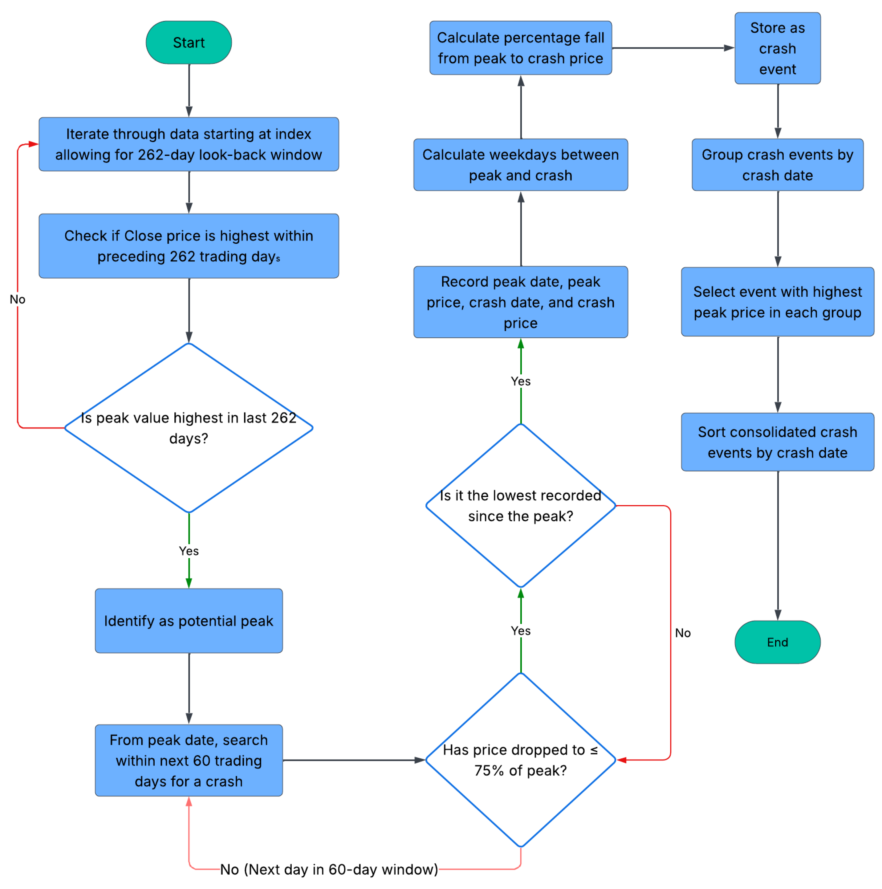
To identify the bubble and crash using the above-mentioned conditions, Historical data of BMV/IPC has been filtered by applying the three conditions. The algorithm in the Figure 1 is followed, and implemented using the Python-3.12. programming Language. The LPPL model will be implemented for each of the crash events in order to calibrate the model. The bubbles and crashes following them are found in the historical data of the index.
These rules are used only to define the historical cases for calibration and evaluation; the LPPL fits itself with cutoffs that stop before the identified crash, ensuring ex-ante evaluation.

3.3. Log-Periodic Power Law

The Johansen–Ledoit–Sornette (JLS) model, also known as the Log-Periodic Power-Law (LPPL) model (Johansen et al. 1999), is a nonlinear framework that helps predict possible stock market crashes by identifying speculative bubbles and estimating the critical time at which such bubbles may collapse (Sornette 2003). By fitting the LPPL function to market prices, researchers capture both the faster-than-exponential growth and the log-periodic oscillations characteristic of bubble dynamics. Although effective, the LPPL model is difficult to calibrate due to its strong nonlinearity and sensitivity to initial parameters (Brée and Joseph 2013).
y ( t ) = A + B ( t c t ) β 1 + C cos ω log ( t c t ) + ϕ
Here, y ( t ) represents the logarithm of the asset price at time t, which stabilises variance and improves numerical fitting.
The LPPL model includes seven parameters (Table 1), out of which three are linear (A, B, C) and four are nonlinear ( t c , β , ω , ϕ ). The nonlinear components are the main focus of LPPL calibration since the linear parameters can be readily solved by regression after the nonlinear parameters are estimated.

3.4. Log-Periodic Power-Law (LPPL) Fitting Method

Prices move up more quickly and fluctuate with decreasing cycles before a break during a speculative run-up. Both components are captured by the LPPL curve: (i) a climb that is quicker than exponential and aiming towards a ceiling; and (ii) little oscillations that are shorter in duration with time. The LPPL equation used for curve fit is
p ( t ) = A + B ( t c t ) β + ( t c t ) β C 1 cos ω ln ( t c t ) + C 2 sin ω ln ( t c t )
In this expression, p ( t ) denotes the observed market price (or log-price) at the trading-day index t, which is the series being fitted to identify bubble-like behavior. The amplitude–phase transformation of the original ( C , ϕ ) representation presented in (Johansen et al. 2000) and covered in (Sornette 2003) is represented by the parameters C 1 and C2, were C 1 = C cos ϕ and C 2 = C sin ϕ . This ( C 1 , C 2 ) variant improves numerical stability during calibration (Filimonov and Sornette 2013). Here, t c is the predicted critical time expressed in trading-day units. As t t c , the factor ( t c t ) β 0 , causing the oscillatory terms to vanish and the trajectory to approach the limiting value A. In this equation, A is the limiting level the curve approaches, B < 0 sets the strength of the accelerating rise, β ( 0 , 1 ) shapes the curvature of that rise, ( C 1 , C 2 ) scale the oscillations, ω says how “fast” the oscillations tick on a log-time axis, and t c is the model’s critical time at which the crash is expected (often a peak or sharp correction). These parameters are listed in Table 1.

3.4.1. Fit Computation

The LPPL curve is fitted to the observed series y ( t ) , where y ( t ) denotes either the raw price P ( t ) or the log-price log P ( t ) . For each time point t i , y ( t i ) is the observed market value and p ^ ( t i ; θ ) is the LPPL model’s predicted value; the residual r i ( θ ) therefore measures their difference. For the parameter vector θ = ( A , B , β , C 1 , C 2 , ω , t c ) , the residual at time t i is
r i ( θ ) = y ( t i ) p ^ ( t i ; θ ) .
Calibration is performed using bounded nonlinear least squares via the trust-region reflective algorithm in SciPy’s least_squares (Virtanen et al. 2020). Trial solutions with t c t i are penalized so that the estimated critical time always satisfies t c > t i .
min θ B i = 1 n r i ( θ ) 2 s . t . t c t i > 0 i .

3.4.2. Bounds and Ex-Ante Constraint (Trading Days)

In order to avoid bad fits, the critical time is constrained to lie just beyond the window end in trading days and set empirically established bounds (Filimonov and Sornette 2013; Sornette 2003). The bound set utilized in the price and log-price variations is compiled in Table 2. We employ data-scaled limits (tighter for log-price) for ( A , B ) in order to enhance conditioning while maintaining B < 0 .

3.4.3. Initialization

To ensure stable LPPL calibration, each nonlinear least-squares iteration begins from a simple and robust data-driven initial vector. The initial values are based directly on the data in the window:
A 0 = median ( y t ) , B 0 = 0.1 stdev ( y t ) ,
β 0 = 0.5 , ( C 1 , 0 , C 2 , 0 ) = ( 0.05 , 0.05 ) ,
ω 0 = 8.5 , t c , 0 = t end + 30 trading days .
This is recommended for stability (Filimonov and Sornette 2013). It usually produces more stable LPPL fits.

3.4.4. Ensuring Feasible Starting Values

LPPL parameters must lie within meaningful ranges, so we define the feasible parameter box:
B = [ A , u A ] × [ B , u B ] × [ 0.1 , 0.9 ] × [ 1 , 1 ] × [ 1 , 1 ] × [ 6 , 13 ] × ( t end + 1 , t end + H td ) ,
This box corresponds to the parameter set ( A ,   B ,   β ,   C 1 ,   C 2 ,   ω ,   t c ) .
Here,
  • A and u A are the lower and upper allowed values for the parameter A (baseline level). These bounds are scaled according to the underlying price series (raw or log).
  • B and u B are the lower and upper allowed values for the parameter B (power-law strength). These bounds are also data-dependent.
  • denotes the vector of all lower bounds: ( A , B , 0.1 , 1 , 1 , 6 , t end + 1 ) .
  • u denotes the vector of all upper bounds: ( u A , u B , 0.9 , 1 , 1 , 13 , t end + H td ) .
The bounds ( A , u A ) and ( B , u B ) depend on whether the model uses raw or log-prices (see Table 3).
The initial parameter vector is:
x 0 = ( A 0 , B 0 , β 0 , C 1 , 0 , C 2 , 0 , ω 0 , t c , 0 ) .
Before optimization starts, x 0 is clipped so that every component lies inside the allowed bounds:
x 0 min ( max ( x 0 , ) , u ) .
This step guarantees that the optimizer starts at a **feasible and meaningful** starting point every time. It prevents issues such as selecting an incorrect critical time (such t c inside the window) or generating extreme parameter values that lead to numerical instability.

3.4.5. Windowing, Selection, and Reporting

Terminal windows of L { 180 ,   240 ,   300 ,   360 ,   420 } (trading days) are fit in both raw price and log-price variants. When a single display window is required, the “common” window is chosen by the lowest mean RMSE across the two variants. For each fit, the model gives R 2 , RMSE, MSE, MAE, and the implied t c as both a trading-day index and its mapped calendar date (nearest trading day in the sample).

3.4.6. Rolling Ensemble (Trading-Day Lead) and Early-Warning Mapping

Ex-ante warnings are generated by advancing the window endpoint over the last 120 trading days in 15 day increments, and calculating the price and log-price for each endpoint fit L { 180 ,   240 } . Only fits that meet the criteria ( 0.1 < β < 0.9 , 6 ω 13 , B < 0 ) are kept. The median is used to aggregate the approved t c values (in trading days) at each endpoint. The trading-day lead time is defined as follows: Δ td = t c med t end .
Bands utilized in the early-warning panel are matched to risk:
Very High if Δ td 7 , High if 7 < Δ td 14 , Elevated if 14 < Δ td 30 .
Bands are displayed as shaded spans centered on each endpoint date (for readability, spans are shown in calendar time but computed from trading-day thresholds). This ensemble reframes LPPL from a single-date predictor into a practical hazard indicator, consistent with robust calibration practice (Filimonov and Sornette 2013).

3.4.7. Bounds and Sign Constraints

All parameters are box-constrained during optimization. Table 3 summarizes the bounds used in the implementation.
Here p 5 , p 95 are within-window percentiles and σ y is the within-window standard deviation. A strict sign filter B < 0 is enforced post-fit to focus on faster-than-exponential regimes.

3.4.8. Code Implementation Algorithm

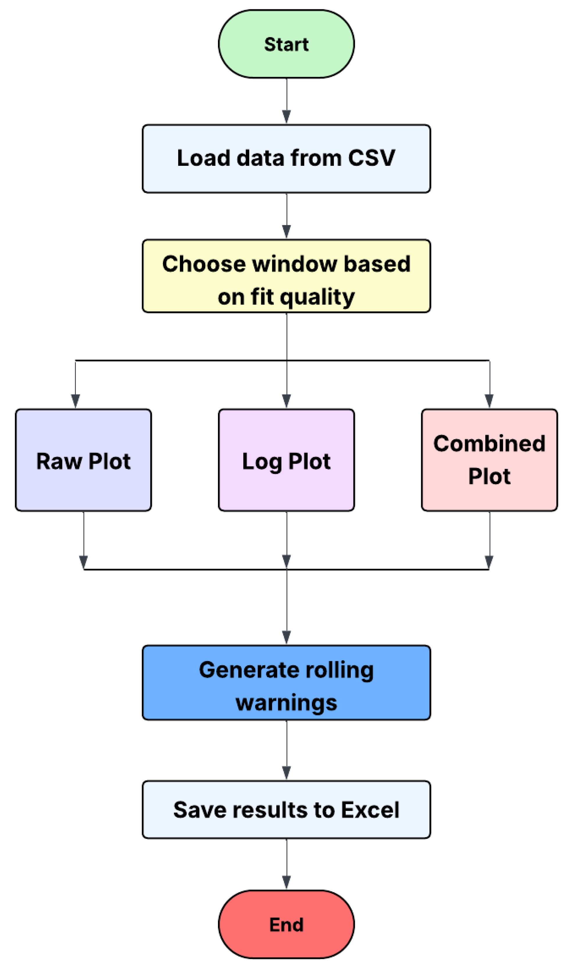
The algorithm given in Figure 2 has been used to implement the LPPL fitting for both the log-price data and the raw price data using the LPPL model.
  • Implementation note
All seven parameters ( A ,   B ,   β ,   C 1 ,   C 2 ,   ω ,   t c ) are estimated jointly via single-stage bounded NLS with the ( C 1 , C 2 ) parameterization (Filimonov and Sornette 2013). The functional form is the standard LPPL equation (Johansen et al. 2000; Sornette 2003); only the time scale (trading-day index) and the oscillatory-term parameterization differ from some expositions.

3.5. LPPL Model Calibration

For calibrating the LPPL model, the study has done the LPPL fitting for each of the crashes identified using the conditions mentioned above. The timeline for each crash case has been taken in the following order:
  • Case 1: From the start of the data to the date of the 1st crash
  • Case 2: From the next day of crash 1 to the date of the 2nd crash
  • Case 3: From the next day of crash 2 to the date of the 3rd crash, and so on.

3.6. Plotting Conventions Used

  • Raw panel: Price in black; LPPL fit in red.
  • Log panel: log-price in green; LPPL fit in orange.
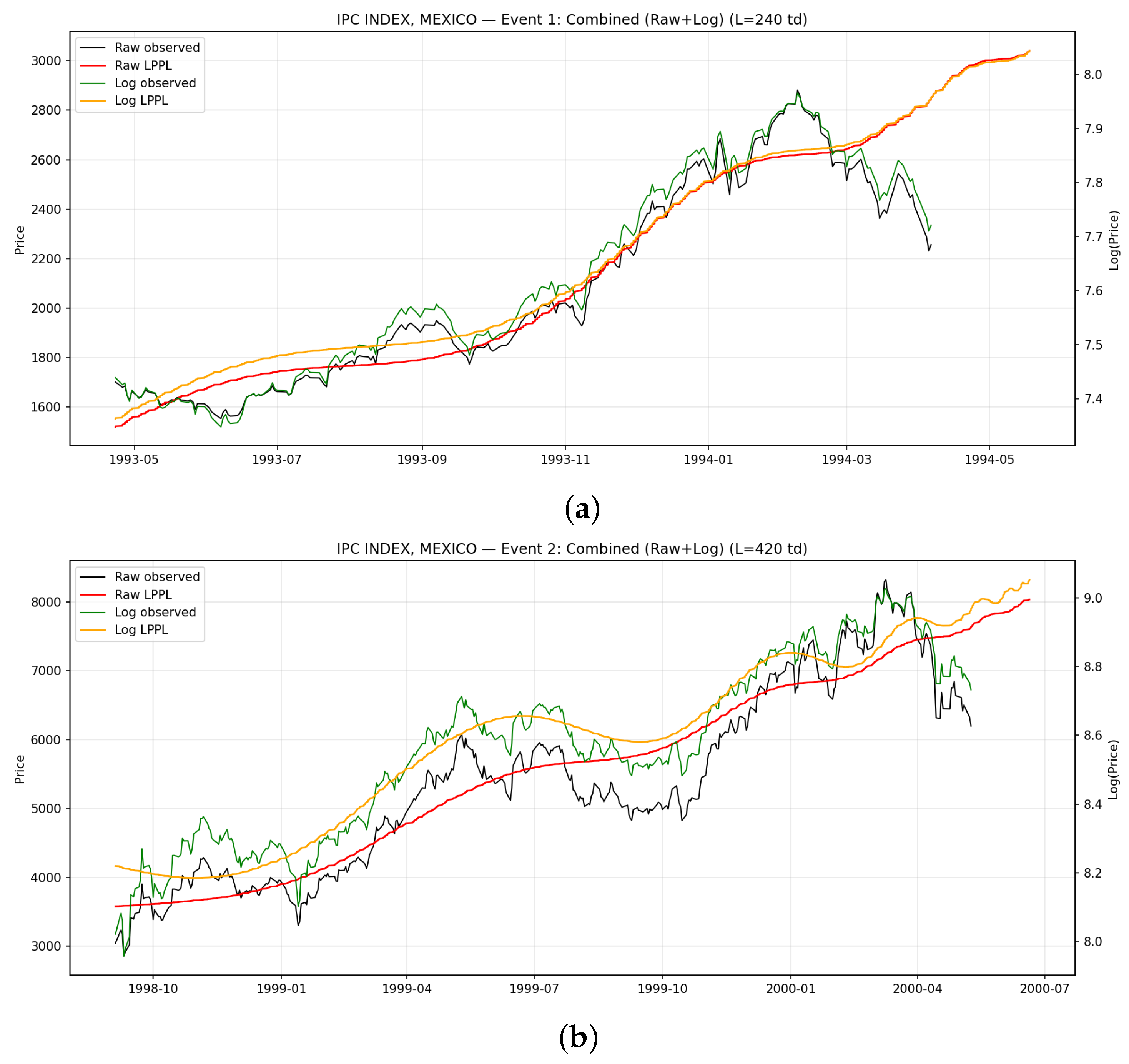
  • Combined panel: Raw (black) + raw LPPL (red) on the left axis; log (green) + log-LPPL (orange) on the right axis.
  • The fitted curve is drawn only up to min t end + Δ , t c , i.e., it never crosses the singularity at t c (Sornette 2003).
  • To avoid ex-post anchoring, no vertical t c line is drawn in the first three panels; timing information is conveyed in the rolling early-warning panel.

3.6.1. Rationale for Dual (Raw/Log) Views

The log transform is recommended for fitting because financial prices often exhibit multiplicative noise and relative changes are more informative than absolute changes; the raw-price view is retained because stakeholders frequently interpret predictions in price units (Cont 2001; Sornette 2003). Showing both helps assess fit stability (log) and practical relevance (raw).

3.6.2. Time Scale and Smoothing Notes

All timing logic (window length, lookback, step, and the t c horizon) is implemented in trading days. Calendar dates appear on the horizontal axes for readability and when reporting the mapped t c date. For the rolling panel, the price curve is lightly smoothed (EMA in event mode; weekly mean in full-timeline mode) to improve readability without altering fit results (Filimonov and Sornette 2013).

3.7. Model Validation

To check the reliability of the LPPL estimates, we apply the following validation steps:
  • Blocked cross-validation: The series is divided into contiguous train–validation segments (not random folds) to preserve temporal order. Each fit is trained on past data and evaluated on a later block, reducing look-ahead bias and helping assess out-of-sample stability (Bergmeir and Benítez 2012).
  • Visual inspection: Fitted LPPL curves are compared with the observed series to verify that the model captures the accelerating trend and characteristic oscillations expected before a regime shift (Sornette 2003).
  • Residual and stability checks: Residuals are examined for obvious structure or drift. Stability of the critical-time estimate is assessed using the interquartile range
    IQR ( t c ) = Q 0.75 ( t c ) Q 0.25 ( t c ) ,
    which summarizes how tightly the ensemble of accepted fits clusters around a common timing (Filimonov and Sornette 2013).
  • Fit metrics: RMSE, MAE, and R 2 are reported as compact indicators of in-sample fit quality. These metrics assist interpretation but are not used to make point forecasts, since LPPL behaves primarily as a hazard model rather than a price-level predictor.
When a single illustrative window is required, we display the calibration with the lowest mean RMSE across the raw and log specifications.

3.8. Early-Warning Scoring (Event Study)

Bands in the rolling panel are computed exactly as in Section 3.4 (trading-day aggregation and thresholds). An early warning is credited when a High/Very High band appears before the realised event and the median t c lies within the specified (±) trading-day tolerance of the event date.

3.9. Software and Tools

All computations in this study were performed in Python using the standard scientific ecosystem and custom code written by the authors. The workflow relied on (NumPy n.d.) for numerical routines and vectorized array operations, pandas for dataset management, date handling, and resampling (Wes McKinney 2010), and SciPy’s least_squares implementation (trust-region reflective algorithm) for bounded nonlinear fitting of the LPPL model. All figures—including raw/log/combined overlays and rolling early-warning panels—were produced with (Matplotlib n.d.), while XlsxWriter was used to generate structured Excel workbooks containing window-wise parameters and rolling-warning summaries to ensure full auditability. Interactive exploration and iterative calibration were carried out in Jupyter Notebook. The entire analysis runs on a standard CPU-based laptop or desktop, with no requirement for GPU acceleration. This open-source toolchain provides a fully reproducible environment and aligns with current LPPL modeling practice, offering transparent numerical optimization, stable time-series management, and publication-quality visual output.

4. Results and Discussions

4.1. Identified Crash Events and Analysis

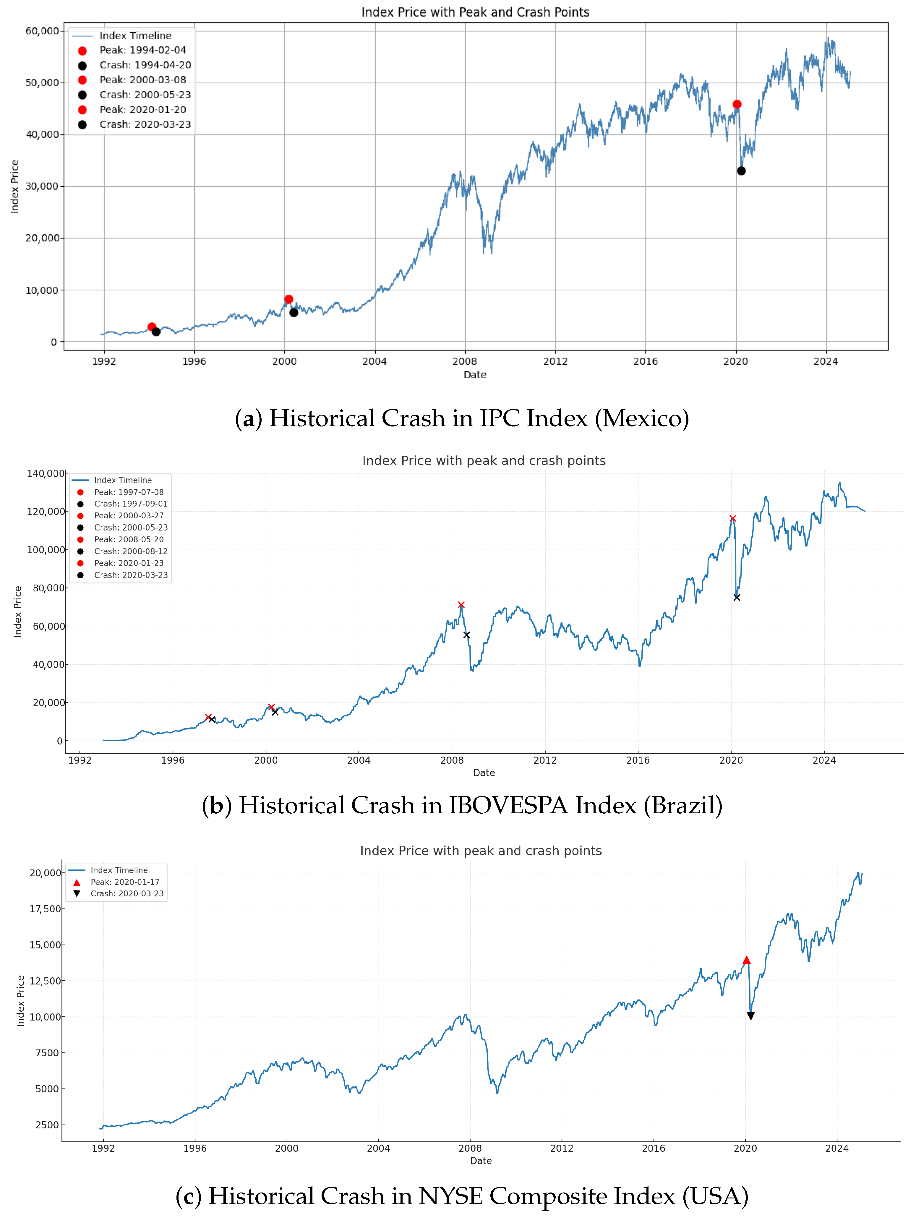
A total of eight major crash events were identified across the three markets, as specified by (Brée and Joseph 2013). These include three events in the IPC/BMV (Mexico), four in the IBOVESPA (Brazil), and one in the NYSE Composite (USA). The complete set of peak dates, crash dates, draw-down magnitudes, and window information is consolidated in Table 4, providing a unified overview of all detected bubble–crash events. A three-panel visualization of the historical price movements for each index is presented in Figure 3 to supplement the tabular summary. Panels (A), (B), and (C) represent the IPC, IBOVESPA, and NYSE Composite, respectively. The marked peak and crash points demonstrate the consistency of the event-identification approach across markets with varying economic circumstances and volatility structures.
Although some major crashes did not meet the criteria, the eight identified crashes are also notable in their respective indexes. These events align with documented market crashes, giving the mechanically identified events external face credibility before the LPPL calibration. The 1994 event (Crash of 1994-04-20) of the IPC (Mexico) is associated with a time of macro and domestic politics instability, the 2000 event (Crash of 2000-05-23), which reflects the global dot-com unwind, which propagated to emerging markets, and the 2020 event (Crash 2020-03-23), which represents the worldwide COVID-19 shock (Shu 2024). In IBOVESPA (Brazil), the 1997 event (Crash 1997-09-01) depicts the effects of the Asian financial crisis, the 2000 event (Crash of 2000-05-23) is associated with the dot-com correction, the 2008 episode (Crash of 2008-08-12) is associated with the global financial crisis and a decline in commodities, and the 2020 event (Crash of 2020-03-23), which is the COVID-19 crash. Last but not least, the COVID-19 collapse is associated with the 2020 event (the crash of 2020-03-23), which is in the NYSE Composite (USA). It is important to note that although the historical timelines for these indices contain other significant crashes, such as the 1997 Asian Financial Crisis, the dot-com bubble burst (2000), the crash following the 9/11 attacks (2001), or the 2008 global financial crisis, they were not identified as ’crash events’ as they failed to meet the three conditions. Only events that strictly fit the description of a rapid and severe descent from a new high were chosen for the study. This was carried out to test and calibrate the model on crash events, which exhibit some uniformity, as each of the identified crash dates satisfied the three conditions given by (Brée and Joseph 2013). This selective approach provides a consistent and objective set of case events for the subsequent testing of the LPPL model.

4.2. Overview of LPPL Fitting on Identified Crash Events

For each of the eight identified crash events, the modified Log-Periodic Power-Law (LPPL) model (Filimonov and Sornette 2013) is fitted on a trading-day time axis using robust multi-start nonlinear least squares. Fits are computed on rolling windows of length L { 180 ,   240 ,   300 ,   360 ,   420 } trading days under the constraints B < 0 , 0.1 < β < 0.9 , and 7 ω 12 . Both raw-price and log-price variants are estimated: the former preserves economic scale, while the latter stabilises variance and typically yields smoother oscillatory components and tighter clustering of estimated critical times t c . Model credibility is assessed by the consistency of t c across windows and by the pattern of rolling early-warning signals.

4.2.1. IPC Index, Mexico

The IPC/BMV index exhibits three major bubble–crash episodes over the sample: the 1994 crisis, the 2000 dot-com spillover, and the 2020 COVID-19 crash. Event 1 (1991–1994) shows a strong rise in 1993 that was followed by increasing instability due to internal political shocks and rising interest rates in the United States. Event 2 (1994–2000) coincides with the global dot-com boom and subsequent unwind, during which external financial conditions transmitted stress to Mexican equities. Event 3 (2018–2020) shows the sharp downturn that followed the COVID-19 pandemic, which was influenced by pressure on global liquidity, falling oil prices, and major Mexican peso selling. For each event, the LPPL analysis evaluates the multi-window fits, selects a baseline specification, and examines the rolling early-warning behavior leading into the observed break.
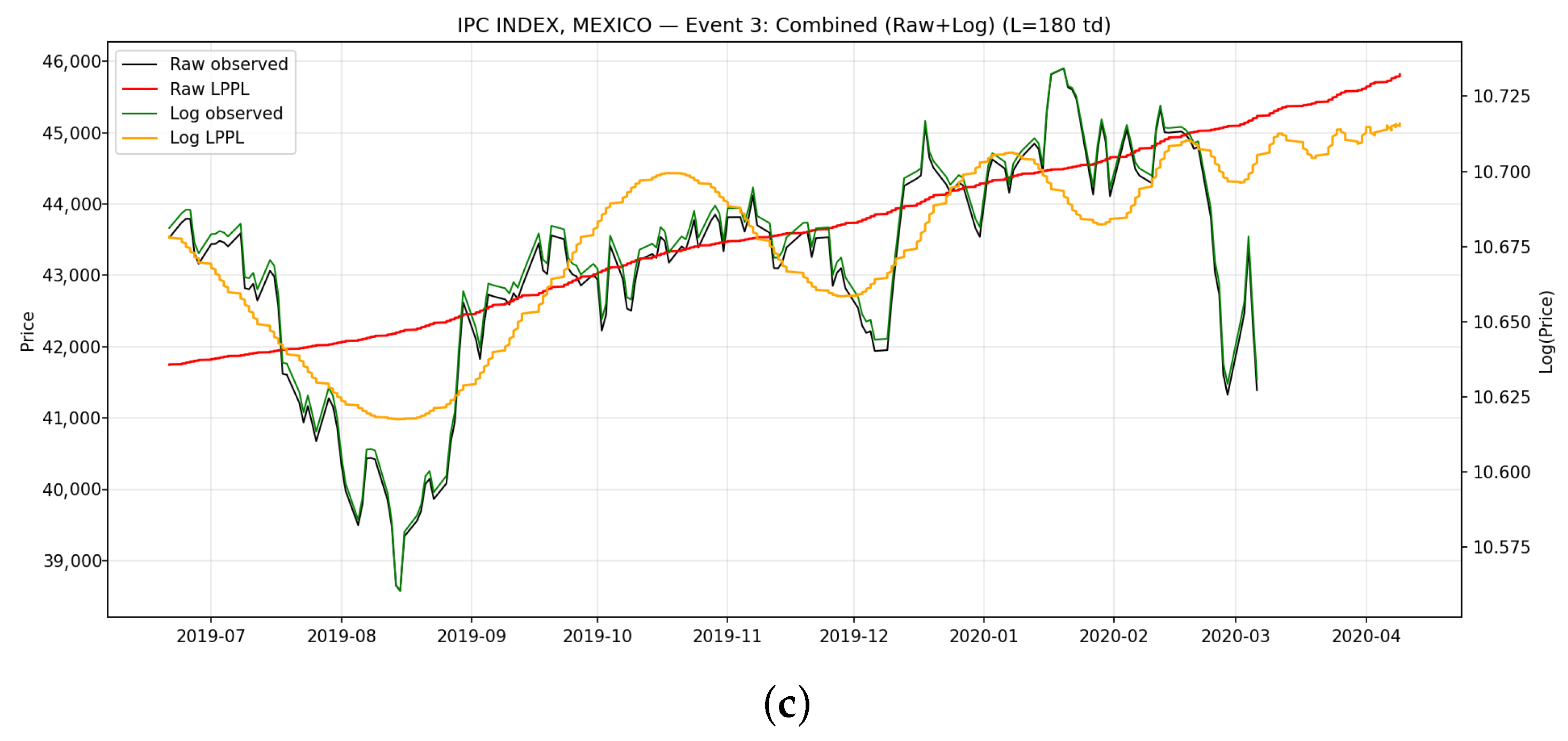
Across the three IPC events, the baseline calibrations presented in Table 5 show a consistent trend: log-scale fits clearly beat raw fits in both accuracy and stability. Event 1 (L = 240) produces strong and balanced fits, with log achieving the highest R 2 (0.9025) and a t c only slightly beyond the actual break. Event 2 (L = 420) yields the best overall explanatory power, with the log variant reaching R 2 = 0.914 and placing t c within a few weeks of the 2000 crash. Even though Event 3’s raw fits are weaker due to the external COVID-19 shock, the log baseline (L = 180) continues to produce a reliable signal with minimal errors and a t c consistent with the March–April 2020 crash window. Overall, the table indicates that log specifications give the most reliable LPPL evidence across all three episodes.
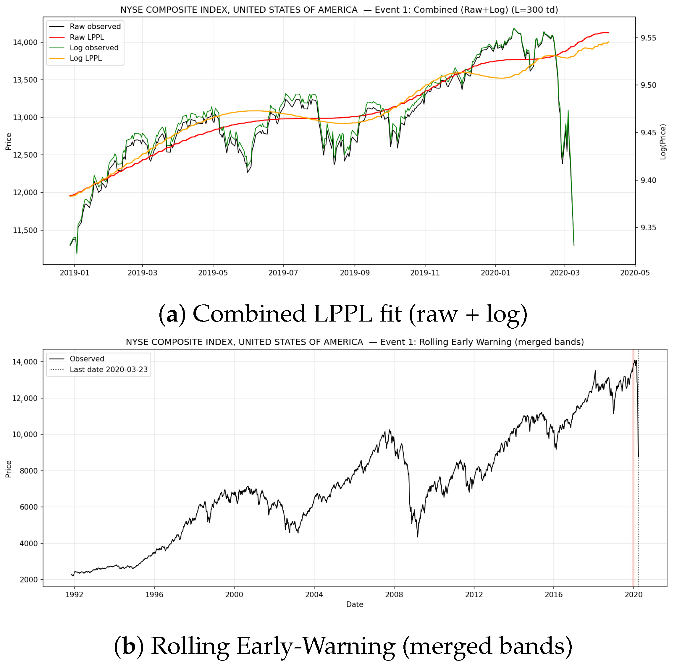
The combined LPPL graphs (raw + log) for the three IPC Mexico events exhibit a uniform bubble formation pattern characterized by faster-than-exponential growth followed by a noticeable reduction of curvature as each crash draws closer, as shown in Figure 4. The combined curve for Event 1 (1994) clearly shows the early 1994 flattening, corresponding with the reversal in April, and the progressive acceleration in 1993. The combined graph nevertheless shows the typical LPPL rising and cresting behavior before the May 2000 dot-com-related break, with the fitted peak falling roughly around the observed crash timeframe, even if Event 2 (2000) shows a longer, more turbulent expansion. Event 3 (2020), although dominated by an external COVID-19 shock, exhibits a gradual LPPL-type curvature through late 2019 and early 2020, indicating rising fragility before the March collapse. Overall, the three panels show that the LPPL structure seems resilient in both externally exacerbated downturns and endogenous build-ups.
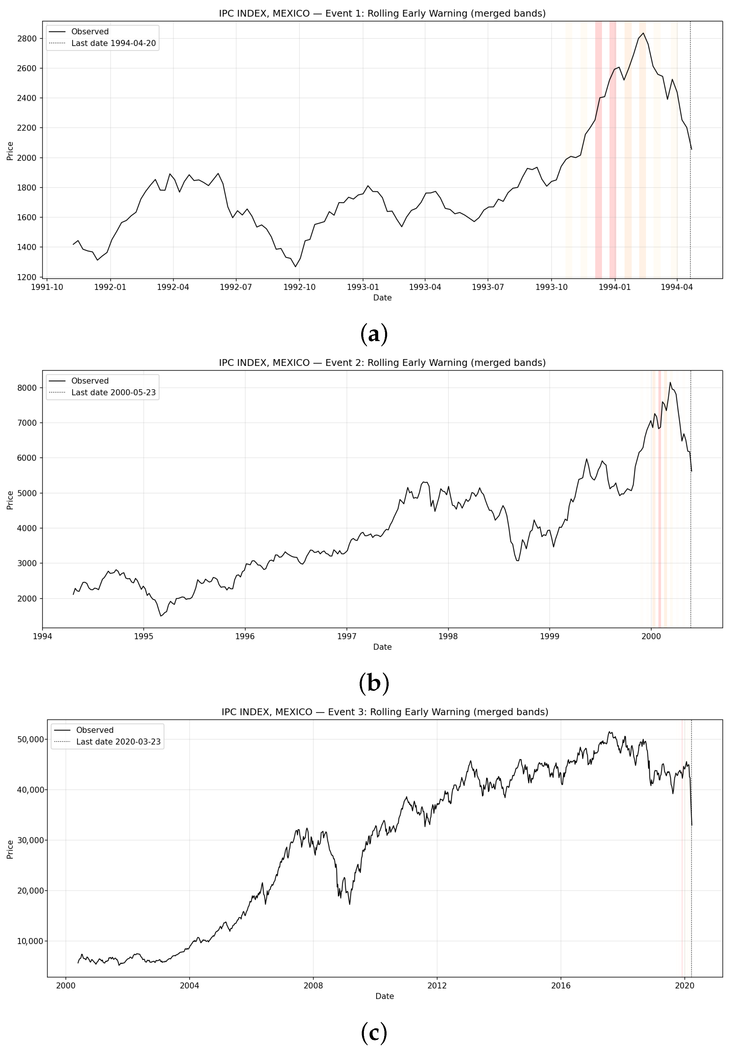
Despite the different macro factors of the three Mexican crashes, the rolling early-warning results for Events 1–3 (Figure 4 and Figure 5; Table 6) demonstrate a consistent LPPL-based buildup of risk. Event 1 demonstrates a typical endogenous bubble: during November and December 1993, warnings increase from Elevated to Very High, and within a few days of the breach on 20 April 1994, they cluster together. The rolling bands show a significant pre-crash acceleration that coincides with the convergence of median t c estimates between late December and early February. During the global tech boom of late 1999 and early 2000, Event 2 shows a larger, externally reinforced bubble. With Very High signals in mid-January and late-February 2000 and closely clustered t c projections around February–March, four actionable alarms occur precisely inside the 60-day timeframe before the crash on 23 May 2000. Event 3 exhibits LPPL-type instability while being driven by the external COVID shock: Very High warnings in November and late December 2019, followed by many Elevated bands through February 2020, narrow t c to mid-March–early-April, surrounding the collapse on 23 March 2020. Together, these results demonstrate that IPC Mexico repeatedly displayed characteristic LPPL pre-crash acceleration, and the rolling system provided timely, escalating alerts—strongly aligned with each subsequent market reversal.
Table 7 shows that, for all three IPC events, log specifications systematically outperform raw fits, with higher R 2 , smaller RMSE, and well-behaved β and ω . The projected t c values closely cluster around the actual crash dates (April 1994, May–June 2000, and March–April 2020) across window lengths, indicating the LPPL calibration’s internal resilience. Although log models continue to indicate a cohesive crucial window, raw fits significantly worsen for Event 3, indicating that LPPL structure endures even throughout the COVID-19 shock event.

4.2.2. IBOVESPA Index, Brazil

For Brazil’s IBOVESPA index, four major crash events are examined, each embedded in a distinct global and domestic context. Event 1, which began on 5 March 1993 and concluded on 1 September 1997, corresponds with growing stress preceding the Asian financial crisis; the late-summer sell-off is consistent with emerging-market risk aversion spreading to Brazil. Event 2, which spans from 2 September 1997 to 23 May 2000, peaks just after the peak of the global dot-com market, following the devaluation of the BRL in 1999 and a dramatic recovery in EM stocks. Event 3, which spans from 24 May 2000 to 12 August 2008, reverses prior commodity-driven gains in a weakening real environment, aligning the August 2008 fall with the pre-Lehman phase of the global financial crisis. Event 4 shows the COVID-19 crash, which ended on 23 March 2020, when Brazil’s stock market suddenly fell from all-time highs in the face of increasingly tightening international financial circumstances. The following analysis creates rolling early-warning diagnostics, baseline fits, and multi-window LPPL calibrations for each event (summarized for four events in Table 8).
Across all four IBOVESPA events, the selected baselines show strong and internally consistent LPPL structure, shown in Table 9. Log specifications systematically dominate raw fits, with much lower RMSE and higher R 2 (up to 0.978 in Event 1 and above 0.90 in Events 2 and 4), while raw remains acceptable but carries large level-scale errors. In every episode, the estimated t c lies close to the historical break, typically a few weeks after the crash, matching the LPPL interpretation of t c as the end of the bubble regime rather than the exact price peak. Using long horizons (360–420 TD) also gives comparable baselines across crises, indicating stable parameters and a persistent LPPL signature in the Brazilian market over 1997, 2000, 2008, and 2020.
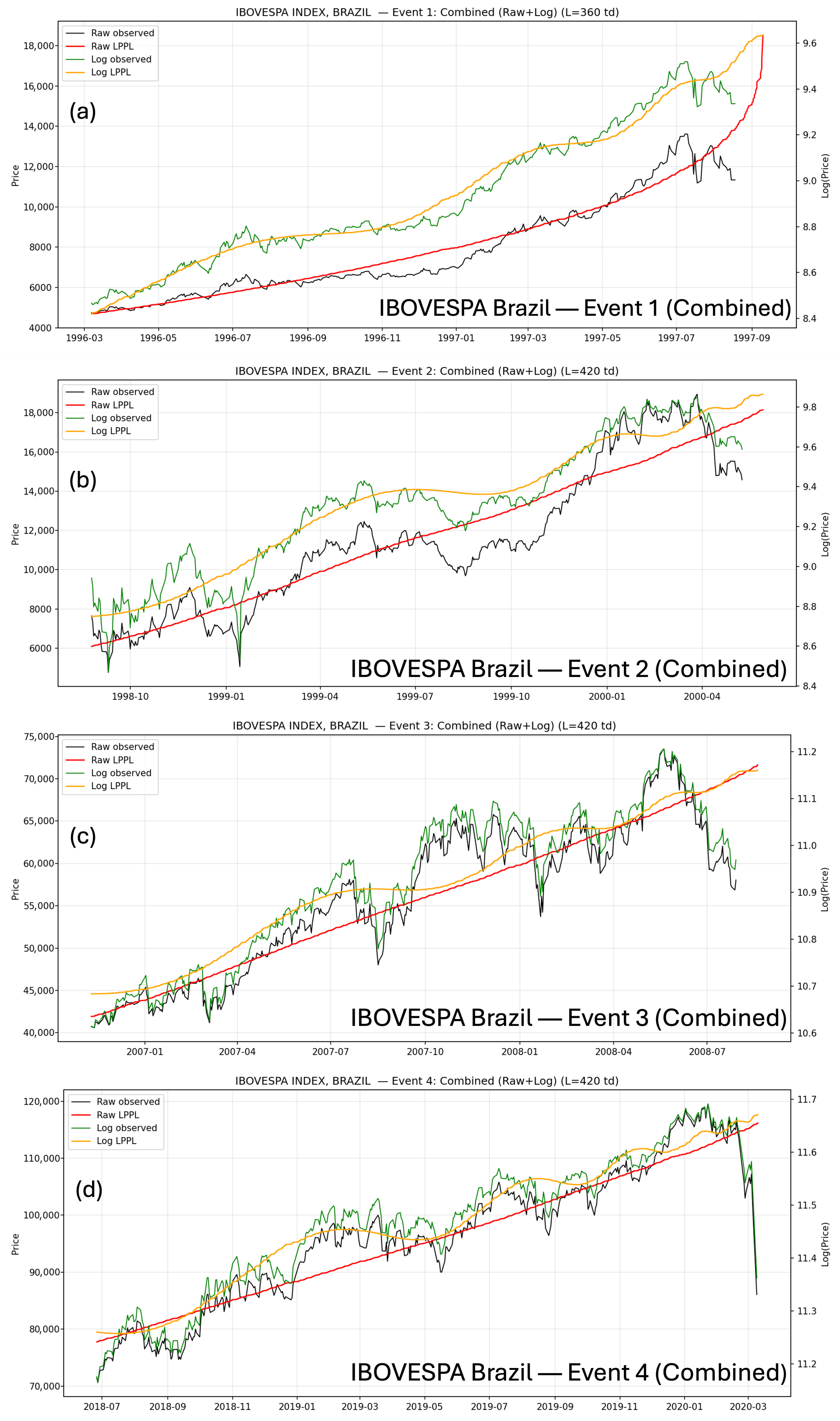
The combined LPPL graphs shown in Figure 6 show a consistent bubble-type acceleration throughout all four IBOVESPA events, with prices following a smooth super-exponential trajectory that flattens and bends as the index draws closer to each crash. In Event 1, the model captures the tightening oscillatory structure leading into the 1997 decline during the Asian crisis spillover. With the LPPL route converging towards the turning point after the strain on developing economies during the dot-com boom, Event 2 demonstrates a distinct run-up towards the 2000 high. Ahead of the 2008 panic, Event 3 shows a clear late-cycle steepening, with the LPPL trajectory accurately bending as global risk aversion increased. The COVID-19 crash represented by Event 4, which exhibits a steady increase through 2019 until a noticeable LPPL levelling just before the bursting in March 2020. When seen together, the four panels show that Brazil consistently displayed LPPL-consistent pre-crash dynamics, with the model’s critical-time curvature appropriately highlighting each bubble phase’s rapid shift.
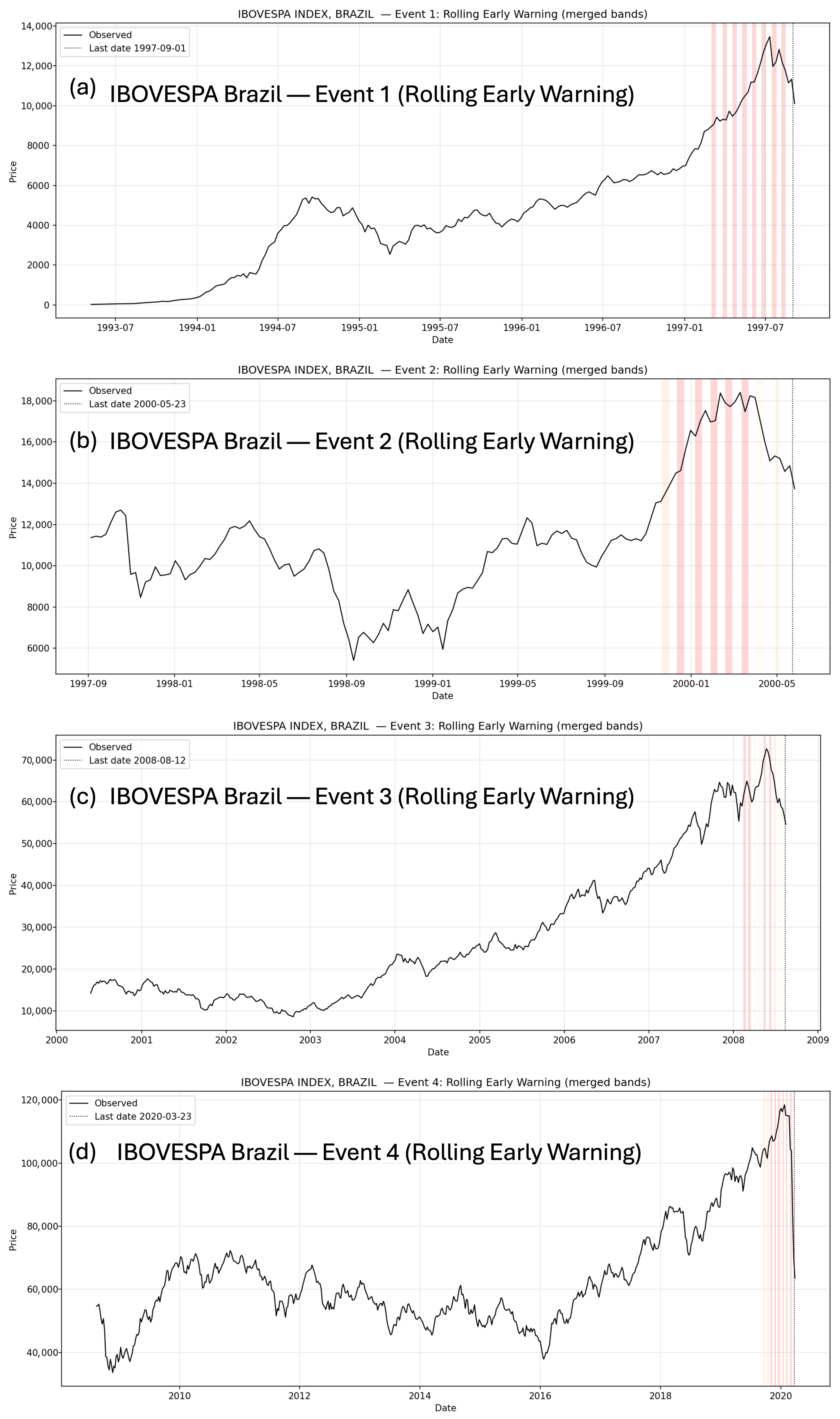
Across all four IBOVESPA events, the rolling early-warning system shows a consistent pattern: warnings begin with moderate lead times and gradually tighten as the market approaches each historical break (Table 10; Figure 7). In Event 1, the model starts flagging instability as early as April 1997, with successive Very High signals clustering through July and August—mirroring the index’s final acceleration ahead of the September sell-off. Event 2 displays an even cleaner structure: risk rises steadily from late 1999, and by early 2000, the windows repeatedly deliver Very High alerts with one-to-three-day leads, capturing the market’s sharp pre-crash curvature during the dot-com period. Event 3 shows a broader buildup, with warnings appearing from February through July 2008; although leads vary, the repeated Very High scans in May–June track the compression in oscillations typical of the late-bubble phase before the global financial crisis. With Very High alerts firing from November 2019 to early 2020, Event 4 displays the densest cluster, reflecting the quick change in mood as COVID-19 transitioned from a localised shock to a worldwide event. When combined, these incidents demonstrate how the LPPL-based rolling system regularly predicts instability by generating dense, short-lead warning clusters right before each significant decline.
Across all four IBOVESPA episodes, the all-window results (Table 8) reveal a remarkably stable LPPL structure. For each event, the logarithmic version systematically outperforms the raw specification: RMSE values fall into the 0.03–0.10 range, and R 2 steadily improves with longer windows, often exceeding 0.85–0.95. In contrast, raw-price models show much larger scale errors but still trace the overall run-up convincingly. The estimated t c values cluster tightly around the known breaks—August–November 1997, late May to mid-June 2000, mid-October 2008, and March–April 2020—despite large differences in market regime and shock origin. This cross-event consistency indicates that each boom phase exhibited a similar super-exponential acceleration, with the LPPL structure remaining detectable across all window lengths.
Across all four IBOVESPA episodes, a broadly consistent picture emerges. Each run-up shows a clear pattern of faster-than-exponential growth with increasingly tight oscillations, and in every case, the model’s preferred fits cluster their critical times close to the eventual breaks. The longer-window calibrations generally offer the most stable behavior, while the rolling early-warning scans add another layer of evidence by showing risk bands that tighten in the final weeks before each downturn. Although the macro catalysts differ—ranging from the Asian crisis and the dot-com unwind to the 2008 global stress and the COVID-19 shock—the underlying bubble dynamics are strikingly similar. Taken together, the four events indicate that the Brazilian market repeatedly exhibited a recognisable LPPL structure and that the framework was able to flag mounting fragility ahead of each major correction.

4.2.3. NYSE Composite Index, United States of America—Event 1

The COVID-19 shock is the first “event” that has occurred on the NYSE Composite. The drop from the long sample (8 November 1991–23 March 2020) reaches its climax on that date, which is also the index’s pandemic panic low. The macro driver is clear: the abrupt halt in global activity brought on by COVID-19 containment measures, which was exacerbated by the fall of the oil price in March 2020 and a cash-strapped liquidity situation. In light of this, the analysis shifts to Table 11, LPPL calibrations for each prospective window.
Ten calibrations, including raw-price and log-price versions, with window lengths ranging from 180 to 420 trading days, are summarized in Table 11. The raw variant is consistently outperformed by the log specification over windows (greater R 2 , much lower RMSE/MAE). While the shortest window (180 TD) is obviously weaker (log R 2 = 0.37), the greatest fits cluster around L = 300–360 TD (log R 2 ≈ 0.63–0.65). The goodness of fit increases as the window length increases from 180 to 300 TD and then levels off. Longer/shorter windows drift towards 19 March 2020 and early June, whereas the best log fits (L = 300–360) indicate 8 April 2020 and 27 April 2020. The suggested key timeframes center around late March to late May 2020. Taken together, Table 11 indicates a stable LPPL signal through late-2019/early-2020 with t c estimates that straddle the observed 23 March 2020 capitulation and the subsequent April re-acceleration.
Table 12 shows L = 300 TD as baseline. Within this window, the log fit achieves the lowest RMSE (≈0.0271) and the highest R 2 (≈0.6516), with t c = 08-04-2020. The corresponding raw fit puts t c = 01-06-2020 and is weaker with the R 2 ≈ 0.652 and RMSE ≈ 350.243. Returning to Table 11, log, L = 300 likewise gives the lowest RMSE and highest R 2 among the log windows, but larger windows (360–420 TD) compromise some fit quality for smoothing. In short, for this event, log L = 300 is the sharpest specification: it fits best in-sample and times the approach to the March 2020 crash more tightly than the raw variant. The combined LPPL graph (Figure 8a) provides a clear view of how the NYSE Composite approached its turning point. The fitted trajectory tracks the broad rise and captures the characteristic LPPL curvature as the market accelerates into the final phase of the upswing. As the series moves closer to the anticipated regime-change zone, the curve begins to bend and lose momentum, reflecting the slowdown typically observed near the critical point.
Reading Table 13 alongside Figure 8b makes the timing clear. Initial warnings appear far in advance (“Beyond60”) on 30 September 2019 and 21 October 2019 (leads ≈ 48 and 32 TD), signalling a maturing upswing rather than an actionable timing cue. Signals then tighten into the decision horizon: “Elevated” by 11 November 2019 (lead 26 TD), “Very High” on 3 December 2019 and 24 December 2019 (leads ≈ 2 TD), and continued “High/Elevated” alerts through mid-January and early February 2020 (leads ≈ 8–15 TD). A final “Beyond60” on 2 March 2020 reflects model-inferred instability stretching further out, even as markets were already sliding. In Figure 8b, these bands cluster immediately to the left of the vertical line marking 23 March 2020, illustrating that risks were repeatedly flagged into the crash window (Table 13, Figure 8b).
The NYSE Composite’s Event-1 diagnostics make sense when taken as a whole. The rolling system (Table 13, Figure 8b) displays warnings that grew more intense from November 2019 through February 2020, offering a compact, high-quality log fit with t c soon after the actual trough. In summary, the best-performing configuration is the log version with a 300-day window. The LPPL recorded the rapid but brittle upswing and sent out timely alerts before the COVID-19 disaster on 23 March 2020 (Table 11, Table 12 and Table 13; Figure 8a,b).

4.3. Comparison and Conclusion of Calibration Phase

The LPPL model behaved consistently and likely around the known breaks (1997 Asian/Russia contagion for Brazil E1, 2000 dot-com crashfor Brazil E2 and IPC E2, 2008 global financial crisis (GFC) for Brazil E3, and March-2020 COVID shock for IPC E3, IBOV E4, and NYSE E1) across all calibrations, from IPC (Events 1–3) and IBOVESPA (Events 1–4) to the NYSE Composite (Event 1). With baseline windows of about 300–420 trading days producing the most stable R 2 and reliable t c estimations, the log-price version produced much lower errors and tighter tracking than the raw-price fit in every market. As would be predicted when a smooth LPPL envelope encounters a distinct crash, inferred crucial dates are regularly grouped within days to a few weeks of the observed break/inflection, usually landing shortly after the panic low.
Complementary historical data were supplied by the rolling early-warning process: warnings began as “Beyond60” far in advance of the breaks and became more intense as markets drew closer to their tipping zone, intensifying to Elevated/High/Very High. Each market and event saw this trend, confirming the decision-horizon framework and demonstrating that signals were not unique to any asset or episode.
When combined, the calibration phase provides a clear operational stance for the full-dataset implementation:
  • Prioritise baseline fits on  300–360 TD windows while scanning the wider 180–420 TD range;
  • use bands of tc and rolling risk states (rather than single-date points) for early-warning interpretation;
  • use the log-LPPL as the primary specification with raw fits as a robustness cross-check. Thus, the model is well-suited to go from historical reconstruction to real-time sample monitoring.

5. LPPL Model Application on Full Data Timeline

After it was demonstrated that the LPPL model could accurately represent bubble dynamics and predict crash dates that frequently fell within a 60-day window of actual crash events across eight distinct historical market crashes from the three indices- IPC Index of Mexico, IBOVESPA Index of Brazil, and NYSE COMPOSITE Index of the United States of America. The complete duration of the IPC index is from 8 November 1994 to 30 January 2025. For the IBOVESPA index, the period is from 3 May 1993 to 30 January 2025. The NYSE COMPOSITE index data spans from 8 November 1994 to 30 January 2025. The study aims to identify recurring trends and enhance the model’s robustness in predicting impending market instability by fitting it to the entire dataset. The model’s fit to the entire dataset will be described in detail in the upcoming sections, along with evaluations of the raw and log-transformed price data and the predicted crash timeframe(s) that resulted.

5.1. IPC Index, Mexico

This subsection applies the LPPL procedure to the IPC index using raw and log-prices over L { 180 ,   240 ,   300 ,   360 ,   420 } trading-day windows. It summarizes cross-window regularities, examines a representative L = 240 baseline, and reviews a short-horizon rolling early-warning scan. As previewed below, log-space fits typically outperform raw fits, and longer windows (360–420 TD) yield the most stable timing, with t c concentrated in October–December 2025.
Table 14 reports the full-sample LPPL fits. Log-space fits consistently outperform the raw specification: log R 2 spans 0.148–0.550, whereas raw R 2 is near zero for shorter windows (0.009–0.018) and improves only at L = 360 –420 (0.253 and 0.373). The log RMSE remains tightly grouped around 0.030–0.041, whereas the raw RMSE is several thousand index points due to level scaling. Across all windows, estimated t c values cluster in October–December 2025, and parameters remain within the standard LPPL ranges. Overall, the log specification provides the clearest and most stable evidence of LPPL-type behavior.
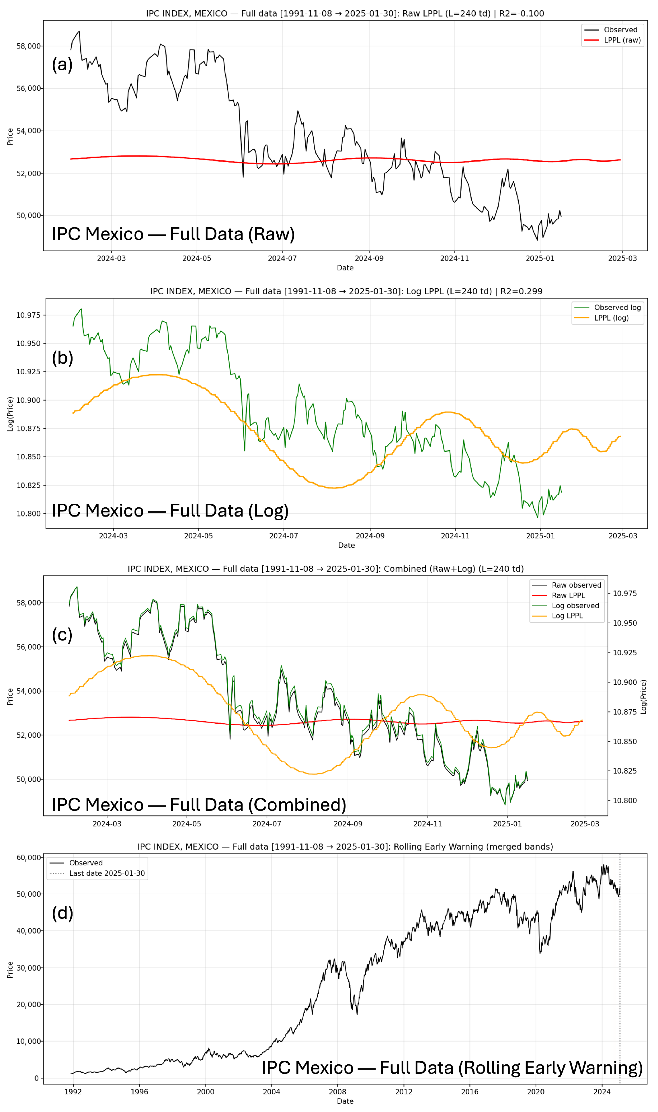
Table 15 presents the L = 240 baseline. Here, the raw fit performs poorly ( R 2 = 0.1000 ), whereas the log fit is materially stronger ( R 2 = 0.2994 ) with a more coherent curvature. The corresponding t c estimates fall in March–April 2025. When compared with the broader L = 180 –420 evidence of Table 14, this baseline is clearly forward-biased: longer windows place t c in late-2025 with substantially higher explanatory power. Thus, the L = 240 slice is retained mainly as a sensitivity check, while the longer log windows (360–420 TD) provide the most credible estimate of the IPC turning point.
Figure 9 shows the L = 240 fits visually. The raw curve reflects the weak R 2 by smoothing over several medium-frequency movements, while the log curve captures the curvature and oscillatory adjustments typical of LPPL. The combined panel makes this distinction explicit, with the log variant aligning more closely with the theoretical structure. This visual contrast mirrors the quantitative gap between the two specifications in Table 15.
Table 16 summarizes the short-horizon rolling scan for 2024–early 2025. All alerts fall into the Beyond60 category, with lead times ranging from approximately 49 to 60 trading days. Signals appear most frequently between August and November 2024, and their median t c values shift gradually toward January–March 2025 as the window advances. Although these do not meet the strict 60 TD action rule, the persistent Beyond60 signals indicate elevated background risk. Their forward-leaning dates do not conflict with the long-window estimates in Table 14; rather, they reflect the shorter-horizon nature of rolling scans versus the more stable long-window calibrations.

5.2. IBOVESPA Index, Brazil

The IBOVESPA index is analyzed using the same structure as for the IPC: an all-window comparison, a representative baseline window, and a rolling early-warning scan. Across all windows, the log specification provides a clearer LPPL signal than the raw version, and the longest window ( L = 420  TD) concentrates the projected t c around mid-October 2025.
Table 17 summarizes the LPPL fits for the IBOVESPA across L = 180 –420 TD. The results display a clear pattern: log-space fits provide consistently higher explanatory power, with R 2 increasing from 0.148 to 0.550 as the window lengthens, while raw fits remain comparatively weak, reaching only R 2 = 0.373 even for L = 420 . Log RMSE is tightly grouped (0.030–0.041), whereas raw RMSE remains several thousand index points. The estimated critical times t c are stable across windows, clustering in October–December 2025, with the L = 420 window centering around mid-October. Longer windows, therefore, reveal a more coherent LPPL structure, especially under the log transformation.
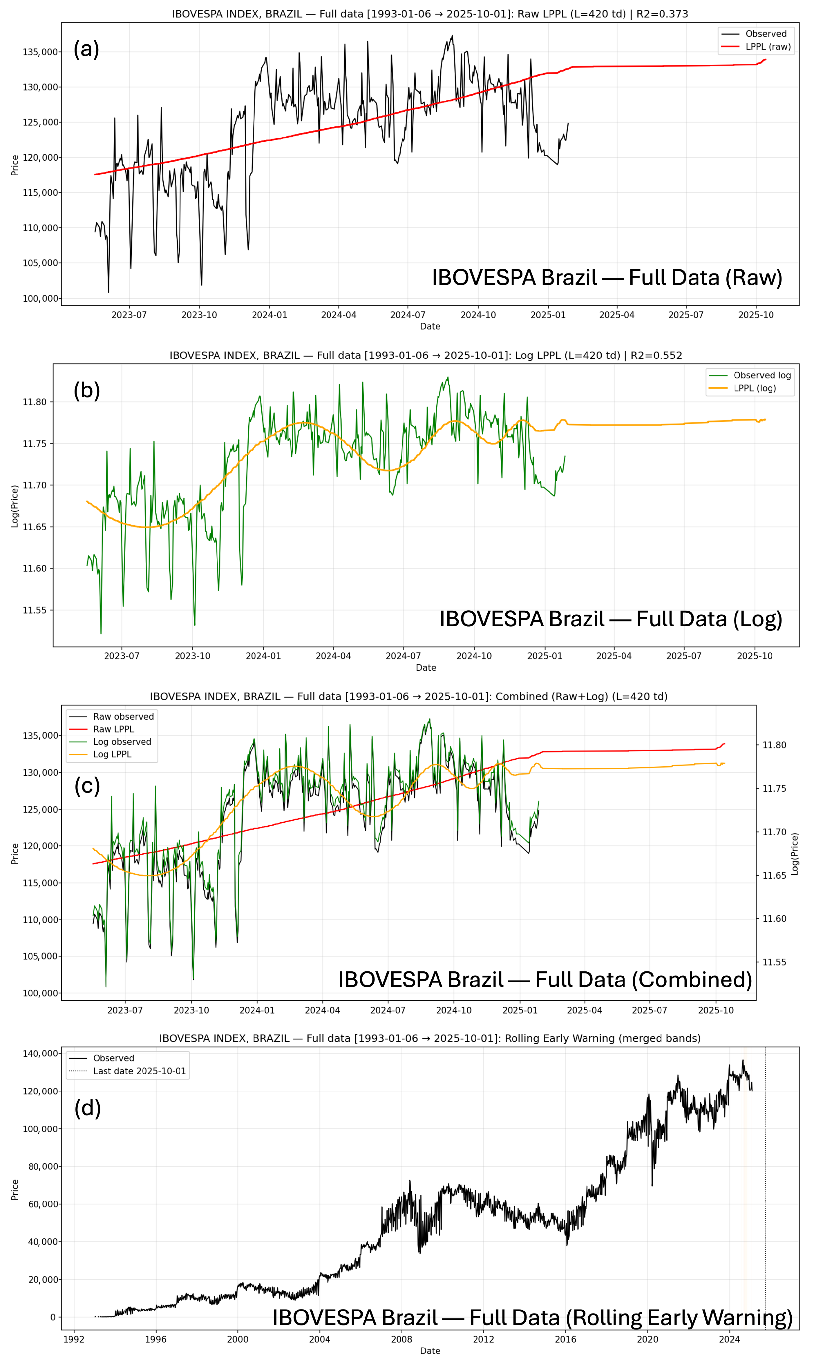
Table 18 presents the selected L = 420 baseline, which produces the strongest fit among all windows. The raw specification achieves R 2 = 0.3730 with t c = 13 / 10 / 2025 , while the log specification attains a substantially higher R 2 = 0.5516 and predicts a nearly identical t c of 14 October 2025. The close agreement in timing reinforces confidence in mid-October 2025 as the likely critical point, while the superior log fit confirms that the transformation improves both curvature and oscillation alignment.
Figure 10 illustrates these differences visually. The raw-price fit (panel a) follows the general trend but misses finer structure, consistent with its lower R 2 . The log-price fit (panel b) captures the mid-2023 dip, the 2024 rally, and the early-2025 consolidation more precisely, matching the stronger log calibration. The combined view (panel c) shows that both variants converge on the same critical window, though the log curve provides the sharper LPPL profile. Together, these results support the use of the log specification for interpreting the IBOVESPA dynamics.
Table 19 reports the rolling-window early-warning alerts. Four windows fall within the strict 60-TD horizon: 28 August 2024 (High risk), 18 September 2024 (Elevated), 10 October 2024 (Very High), and 31 October 2024 (Elevated), offering advance warning through late 2024 (Appendix A). The remaining windows lie beyond the 60-TD threshold but indicate continued sensitivity of the model as the window advances into early-2025. For readability, Figure 10 omits shaded bands, leaving the table to supply precise lead times. Overall, the rolling scan complements the long-window calibration by showing a sequence of short-term tensions ahead of the October 2025 turning point window.

5.3. NYSE Composite, United States of America

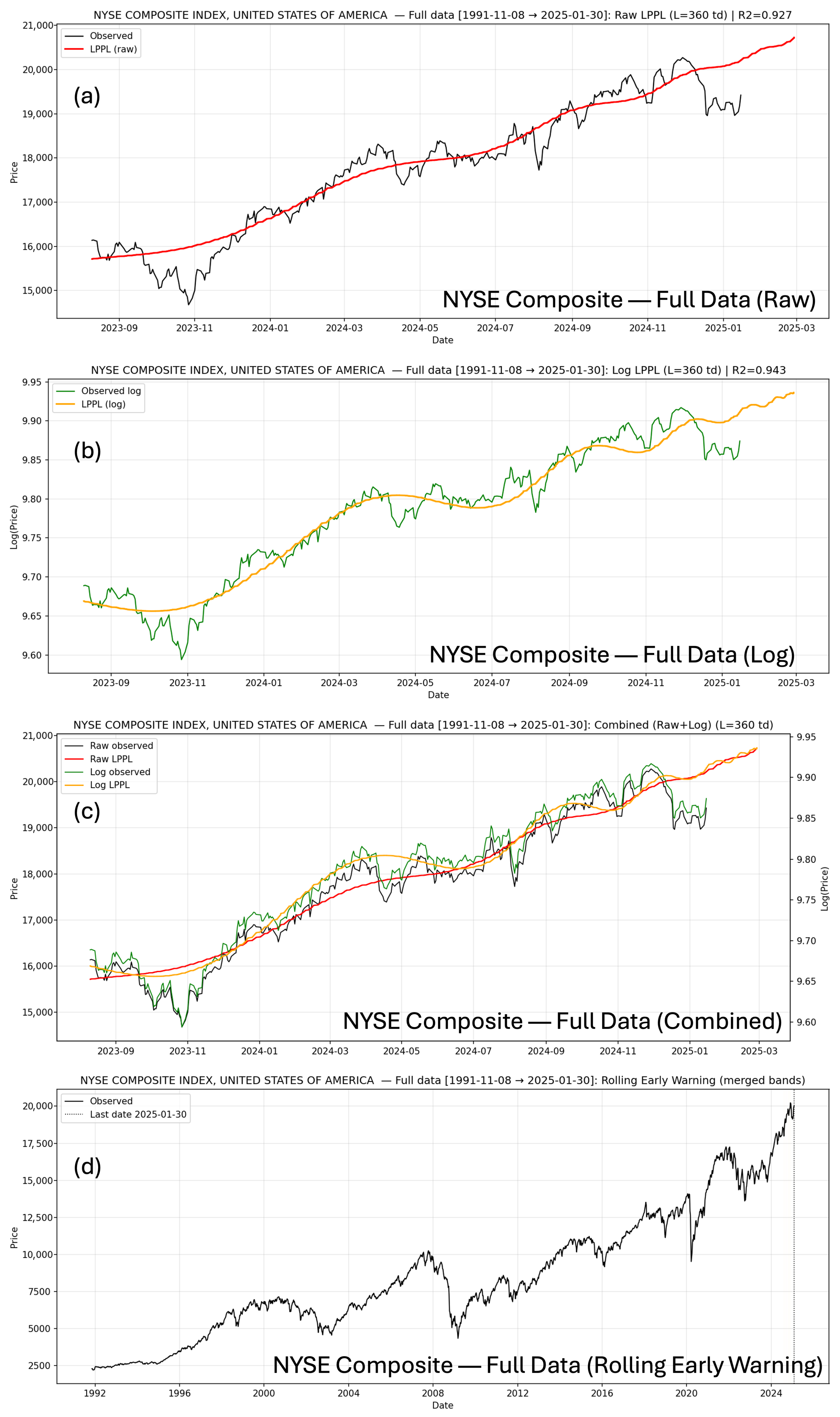
The NYSE Composite is analyzed using the same three-step structure applied to the IPC and IBOVESPA: an all-window comparison, a representative baseline window, and a rolling early-warning scan. As a preview, the log specification provides the strongest explanatory power, and the estimated critical times t c consistently fall in a narrow early March–early April 2025 band. Table 20 shows that both raw and log specifications yield strong fits for the NYSE, but the log variant consistently performs better. Log-space R 2 values rise from about 0.75 at L = 180 to 0.94 at L = 360 –420, paired with very low RMSE values (0.018–0.021). The raw fits also perform well ( R 2 0.72 0.93 ), though at a much larger scale of RMSE in index points. Estimated critical times are highly stable across windows, centring between early March and early April 2025. This consistency across horizons indicates a clear LPPL structure and a well-behaved optimization landscape.
Table 21 presents the selected baseline using the L = 360 window. The raw fit produces a strong R 2 = 0.9269 with t c = 10 / 04 / 2025 , while the log fit improves the explanatory power to R 2 = 0.9431 and identifies a slightly earlier t c of 06/03/2025. The agreement in timing, combined with the superior log fit, reinforces the conclusion from the all-window results that the NYSE was approaching a critical transition in early 2025. Figure 11 illustrates the fit behavior across scales. The log-price LPPL curve (panel b) captures both the accelerating trend and the oscillatory structure visible from 2023 to early 2025, consistent with its high R 2 . The raw-price curve (panel a) tracks the broader movement but is less sensitive to finer fluctuations. The combined panel (c) shows that both variants converge on the same critical window, while the rolling panel (d) presents how instability accumulates toward late 2024. Together, the visuals align with the statistical findings from the tables.
Table 22 summarizes the rolling-window early-warning outputs. Early alerts appear in August and September 2024 with long lead times (40–60 trading days), indicating growing instability well before the January 2025 downturn. By late November and December 2024, the system issues Elevated-risk signals with much shorter leads (14–22 trading days), marking a tightening approach toward the estimated t c . As the rolling window enters 2025, the predicted t c moves beyond the 60-day horizon and becomes more dispersed—an expected behavior when the window approaches the peak itself. Overall, the rolling scan complements the static calibration by showing how risk intensified steadily through late 2024.

6. Discussion

6.1. Synthesis Across Markets and Methods

A broad look across the IPC, IBOVESPA, and NYSE Composite confirms several common patterns in how the LPPL structure emerges across different market environments. One of the clearest themes is the consistent advantage of log-space fitting. In every market, the log specification not only generates higher R 2 values but also produces smoother and more interpretable oscillations that match the expected LPPL shape. This is especially visible in the longer windows, where the combination of a longer lookback and log transformation tends to stabilise parameters such as ω and the estimated critical time t c . The raw-price variant still captures the broad acceleration, but it reacts more strongly to short-run volatility and often exaggerates level effects, which makes it less reliable for timing.
Another unifying feature is the clustering of t c across adjacent window lengths. Instead of producing scattered or contradictory timings, the models converge onto coherent bands: early spring 2025 for the U.S., mid-October for Brazil, and late 2025 for Mexico. These clusters, along with visually stable combined curves, indicate that the bubble regimes in each market are not artefacts of a single parameter choice but persist across a wide range of windows. This type of cross-window agreement is generally taken as a sign of structural LPPL behavior rather than incidental curve-fitting.
Despite the differences in geography, liquidity, and macro context, the three indices show remarkably similar LPPL signatures: sustained super-exponential rises, progressively tightening oscillations, and a clear flattening as the system approaches its predicted critical region. The agreement of these patterns across such different markets strengthens the overall interpretability of the results and suggests that the method is capturing genuine commonalities in speculative dynamics rather than idiosyncratic noise.
Together, these observations match the practical use of LPPL in earlier studies: fit in log space, rely on broader windows for stability, and use multi-window checks to avoid over-interpreting any single calibration. The approach used here follows that logic closely.

6.2. Rolling Early-Warning Signals

The rolling early-warning framework adds a practical, time-sequenced view of how risk builds as markets approach a potential turning point. Rather than focusing on a single fitted window, the rolling approach reveals how frequently and how forcefully different calibrations point toward a critical region. What stands out in all three markets is the progression from scattered, low-intensity alerts to dense clusters of High and Very High warnings as the crash window approaches.
These warnings do not arrive as isolated surprises; they build gradually as the model repeatedly detects compressed oscillations and rising curvature in the price series. For example, in multiple markets, the earliest warnings appear well before the eventual downturn, giving a sense of persistent but still distant instability. As more rolling windows are added and the price approaches the final upswing, the warnings tighten into short-lead clusters—often just a few trading days ahead—which match the visual “curling over” in the combined charts.
Equally important is that the rolling system distinguishes between signals that fall within a realistic decision horizon and those that lie just beyond it. The use of Beyond-60 tags prevents over-interpreting long-lead warnings while still documenting their presence. This makes the framework more transparent and avoids the common criticism that LPPL warnings are either too early or too ambiguous to be useful.
Overall, the rolling results complement the static window fits. Where the static fits show structural LPPL behavior over long horizons, the rolling scans reveal how that structure intensifies in real time, turning a theoretical model into a practical warning tool.

6.3. Comparison with Prior LPPL Studies

The empirical behavior observed across the IPC, IBOVESPA, and NYSE Composite aligns closely with the dominant findings in the LPPL literature. The stronger performance of log-space fits—visible in higher R 2 values, lower RMSE, and clearer oscillatory structure—is consistent with the argument made by (Filimonov and Sornette 2013) that log transformations better reveal multiplicative noise and stabilise the nonlinear phase parameters. The present results also echo (Brée and Joseph 2013), who show that raw-price fits tend to be noisier and more sensitive to local trends, especially in emerging markets.
Across all three markets, the estimated critical times cluster tightly when longer windows are used, which mirrors the t c convergence documented in classic case studies such as Johansen and Sornette’s work on the Nasdaq and FX crises (Johansen and Sornette 1999, 2000). The stability of ω and the presence of sustained log-periodic oscillations across neighbouring windows are also consistent with more recent LPPLS implementations that emphasise parameter constraints and multi-window validation (Filimonov and Sornette 2013; Shu 2024).
The pattern of t c slightly lagging the actual turning point—visible in both the IBOVESPA and NYSE series—is typical in LPPL applications and has been noted repeatedly in empirical studies. This reflects the model’s interpretation of t c as the theoretical limit of the unsustainable phase rather than the exact day of market reversal. The rolling early-warning behavior shown here—broad early signals followed by compressed, high-frequency warnings near the peak—matches this narrative and resembles the escalating hazard structure reported in earlier LPPL analyses of equity and commodity bubbles.
Taken together, the three-market comparison positions the present results squarely within the observed behavior of LPPL models in the literature: stronger log-space structure, clear oscillatory signatures, stable t c clusters, and warnings that emerge in a realistic and actionable time frame before the observed breaks.

6.4. Strengths and Limitations

A notable strength of the LPPL approach, as applied across the three markets, is its ability to impose a behavioral structure on price dynamics rather than treating bubbles as purely statistical anomalies. By modeling prices as the outcome of accelerating herding behavior with characteristic oscillations, the framework produces signals that can be interpreted in economic terms rather than simply as curve-fitting artefacts. This interpretability becomes especially valuable when the fitted trajectories, oscillatory patterns, and the predicted critical time t c all move together in a coherent way across multiple windows, as observed in the IPC, IBOVESPA, and NYSE results.
Another strength lies in the robustness gained from the use of log-space fitting, longer window lengths, and multi-window cross-checking. These elements reduce the tendency of the model to latch onto short-lived fluctuations and instead emphasise the underlying structure of the bubble regime. The relatively tight clustering of t c across adjacent windows—particularly in the NYSE (March–April 2025) and IBOVESPA (around mid-October 2025) cases—illustrates how this layered approach filters noise while still preserving sensitivity to real shifts in market curvature. The rolling early-warning view further complements this by translating structural model outputs into a timeline that investors, analysts, and policymakers can more easily interpret.
However, the method is not without its limitations. LPPL parameters, particularly ω and the phase-related components, are known to exhibit sloppiness: multiple combinations can produce similarly good fits, and small changes in sample boundaries can occasionally shift the estimated critical time. This is mitigated here through constrained optimization and stability checks, but the issue cannot be eliminated entirely. Moreover, the model’s predictive interpretation requires caution. A predicted t c marks the end of the bubble regime rather than a literal crash date; markets often begin turning before or after the inferred t c , and external shocks can accelerate or delay the transition.
There is also an unavoidable sensitivity to window choice. While longer windows tend to stabilise the fits, they may smooth away shorter speculative phases that are nevertheless relevant in real-world decision-making. Conversely, shorter windows can exaggerate brief volatility spikes and pull t c closer than justified by the broader trend. This tension is a longstanding concern in empirical LPPL work and underscores the need for cross-window comparison rather than reliance on a single “best” fit.
Finally, LPPL signals should not be viewed in isolation. Although the model captures characteristic bubble dynamics, real markets are influenced by policy surprises, geopolitical shocks, liquidity breaks, and other events that lie outside the model’s behavioral assumptions. For practical use, LPPL indicators are most valuable when combined with market-internal measures—such as breadth deterioration, credit spreads, or macro sentiment—as a way to avoid false positives and to improve the reliability of early warnings.

7. Conclusions

This study examined whether the LPPL model can identify phases of unsustainable price acceleration, produce stable estimates of the critical time, and offer an early-warning perspective across major equity markets. The results address these objectives directly. For the IPC, IBOVESPA, and NYSE Composite, the LPPL framework—especially in log form and over longer windows—captures the characteristic faster-than-exponential growth and oscillatory patterns associated with speculative bubbles. In all three indices, the estimated t c clusters appear ahead of the downturns identified in the empirical analysis, supporting the model’s ability to recover the main signatures outlined in the research questions.
The findings also connect clearly to the contributions outlined in Section 2.5. The systematic calibration for Mexico shows that LPPL dynamics are present even in a market that has received limited attention in this literature. The multi-window and rolling early-warning procedures demonstrate why single-window estimates can be unreliable in volatile emerging markets and how cross-window checks improve stability. The comparison with Brazil and the United States situates Mexico within a broader regional context, highlighting both shared bubble patterns and market-specific differences. The results also provide a practical framework for risk monitoring, suggesting that LPPL can help regulators and investors recognise when markets enter a high-risk acceleration phase.
Some limitations remain. A few well-known crashes do not satisfy the Brée and Joseph criteria, and certain parameters remain sensitive to window length, particularly when data history is limited. These issues reinforce the view that LPPL is best interpreted as signalling a rising hazard phase rather than offering precise crash dates. Used conservatively and alongside other market indicators, it can nonetheless contribute meaningfully to early-warning assessment.
Overall, the evidence shows that LPPL—when calibrated carefully and validated across multiple windows—can provide timely insight into unstable growth regimes. The cross-market comparison highlights where the model performs well and where its limits appear. Future work could test alternative crash-identification rules, incorporate sentiment or microstructure data, or develop hybrid approaches that combine LPPL’s behavioral foundations with more empirical robustness.

Author Contributions

Conceptualization, S.S., A.K.G., R.M. and V.S.; methodology, S.S., R.M. and V.S.; software, S.S., R.M. and V.S.; validation, S.S. and V.S.; formal analysis, S.S., R.M. and V.S.; investigation, A.K.G., R.M. and V.S.; resources, A.K.G., R.M. and V.S.; writing—original draft preparation, S.S., A.K.G., R.M. and V.S.; writing—review and editing, A.K.G., R.M. and V.S.; supervision, A.K.G., R.M. and V.S. All authors have read and agreed to the published version of the manuscript.

Funding

This research received no external funding.

Data Availability Statement

The original contributions presented in this study are included in the article. Further inquiries can be directed to the author.

Conflicts of Interest

The authors declare that there are no conflicts of interest.

Abbreviations

    The following abbreviations are used in this manuscript:
LPPLLog-Periodic Power Law
TDTrading Days
IQRInterquartile Range
RMSERoot Mean Squared Error
MSEMean Squared Error
R 2 Coefficient of Determination
MAEMean Absolute Error
BMV/IPCMexican Stock Exchange Index
NYSENew York Stock Exchange
IBOVESPA/IBOVBrazilian Stock Market Index

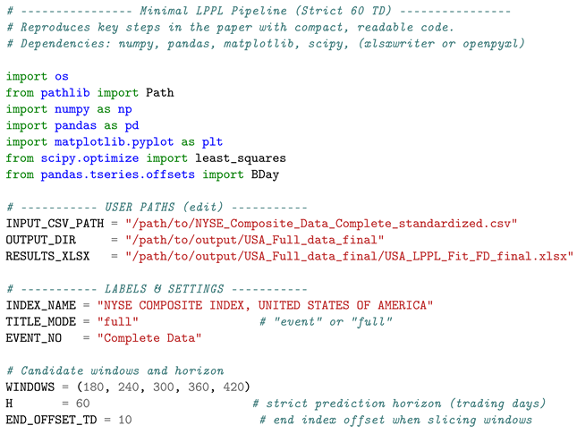
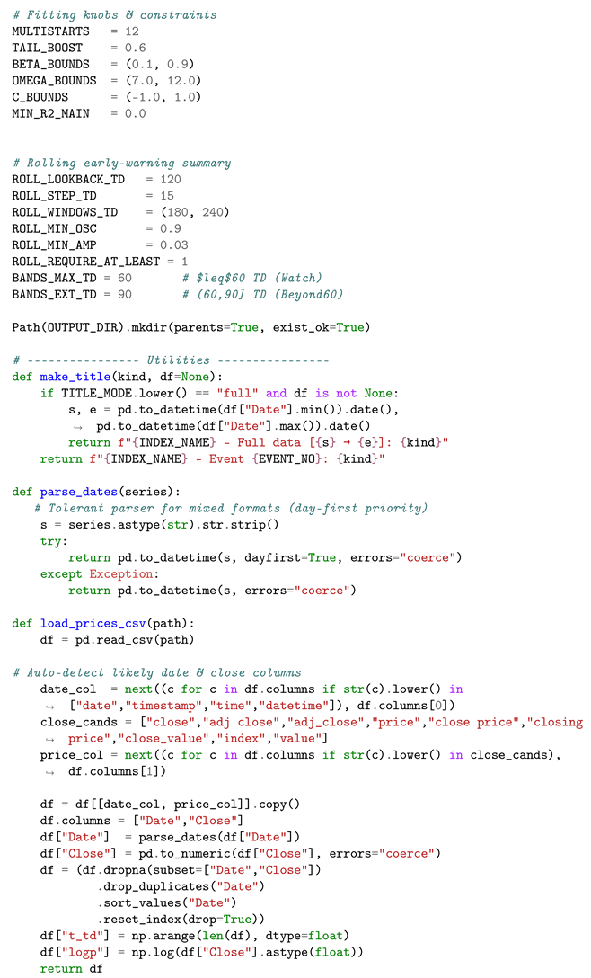
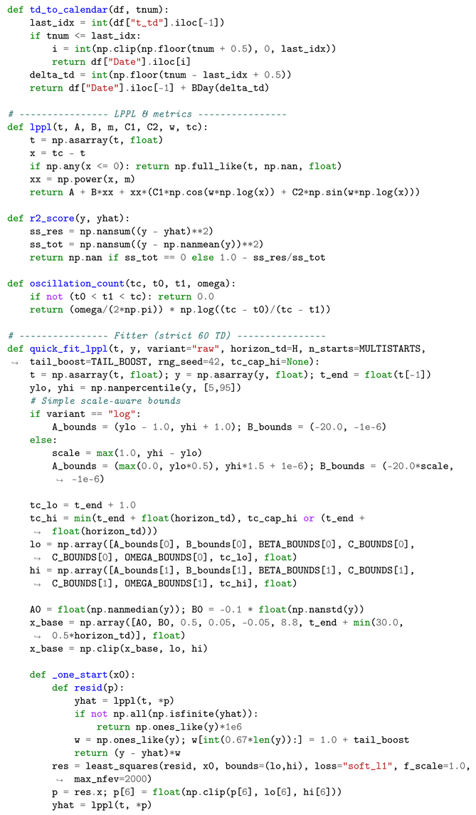
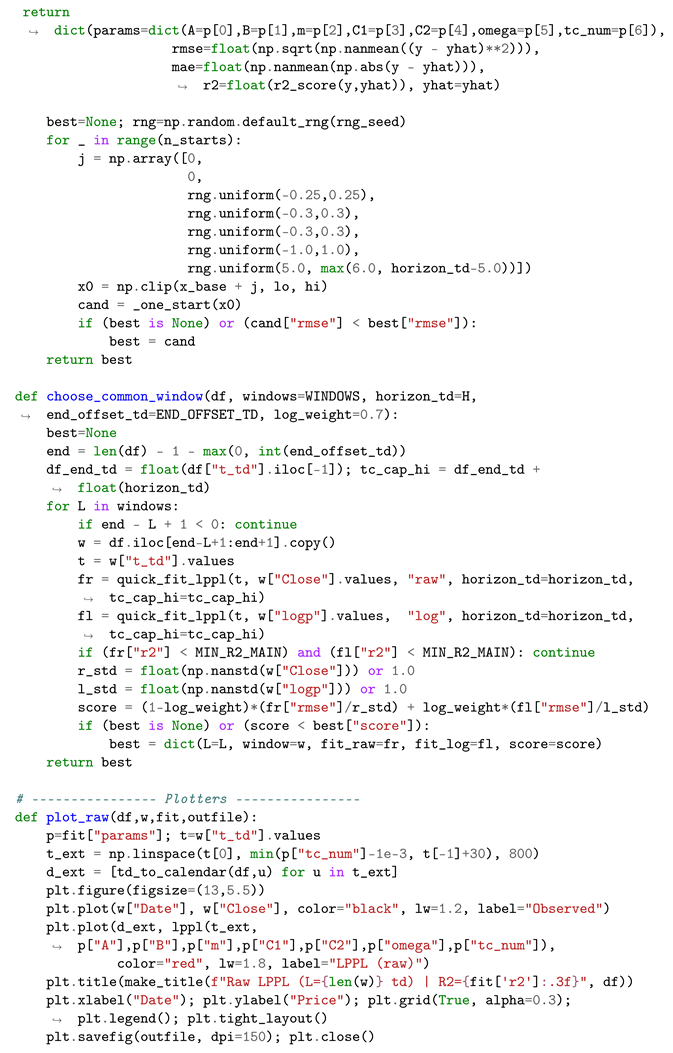
Appendix A. Minimal LPPL Pipeline (Strict 60 Trading-Day Horizon)

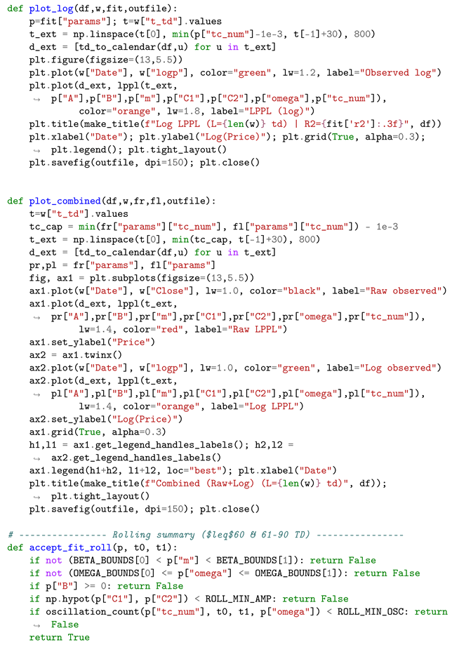
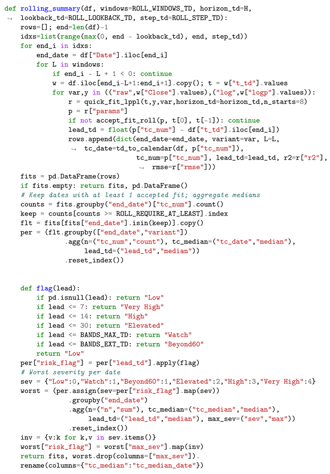
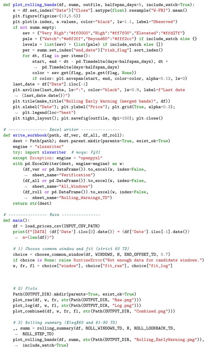
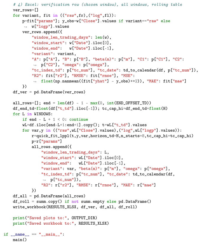
  • Purpose. This minimal, self-contained Python script reproduces the core steps used in the paper: robust date parsing, LPPL calibration on candidate windows with a strict H = 60 trading-day prediction horizon, selection of a common window (raw + log), three publication-quality plots (Raw, Log, Combined), a rolling early-warning summary with merged severity bands (≤60 TD “Watch” and 61–90 TD “Beyond60”), and an Excel workbook with the “Verification”, “All_Windows”, and “Rolling_Warnings_TD” sheets.
  • Dependencies. numpy, pandas, matplotlib, scipy, and optionally xlsxwriter.
Listing A1. Minimal LPPL pipeline used for reproducibility (strict 60-TD horizon).
Risks 14 00003 i001Risks 14 00003 i002Risks 14 00003 i003Risks 14 00003 i004Risks 14 00003 i005Risks 14 00003 i006Risks 14 00003 i007Risks 14 00003 i008
Notes. (i) The script enforces a strict H = 60 trading-day horizon for t c when calibrating each window; (ii) candidate windows L { 180 ,   240 ,   300 ,   360 ,   420 } are scored using a scale-aware blend of raw/log RMSE; (iii) rolling early-warning bands visualize merged severity intervals for “Watch” (≤60 TD) and “Beyond60” (61–90 TD); (iv) the Excel workbook always contains three sheets—Verification, All_Windows, and Rolling_Warnings_TD.

References

  1. Advisors, Covenant Wealth. 2025. Market Corrections: Definition and How Investors Should Respond. Available online: https://blog.commonwealth.com/ (accessed on 25 June 2025).
  2. Bandyopadhyay, Gautam. 2016. Gold price forecasting using arima model. Journal of Advanced Management Science 4: 117–21. [Google Scholar] [CrossRef]
  3. Banjade, Dhruba. 2020. Forecasting bitcoin price using artificial neural network. SSRN Electronic Journal. [Google Scholar] [CrossRef]
  4. Bartolozzi, Marco, Stanislaw Drożdż, D. B. Leinweber, J. Speth, and Anthony William Thomas. 2005. Self-similar log-periodic structures in western stock markets from 2000. International Journal of Modern Physics C 16: 1347–61. [Google Scholar] [CrossRef]
  5. Bergmeir, Christoph, and José M. Benítez. 2012. On the use of cross-validation for time series predictor evaluation. Information Sciences 191: 192–213. [Google Scholar] [CrossRef]
  6. Blanchard, Olivier, and Mark Watson. 1982. Bubbles, Rational Expectations and Financial Markets. Technical Report. Cambridge: National Bureau of Economic Research. [Google Scholar] [CrossRef]
  7. Blanchard, Olivier Jean. 1979. Speculative bubbles, crashes and rational expectations. Economics Letters 3: 387–89. [Google Scholar] [CrossRef]
  8. Brée, David S., and Nathan Lael Joseph. 2013. Testing for financial crashes using the log periodic power law model. International Review of Financial Analysis 30: 287–97. [Google Scholar] [CrossRef]
  9. Chai, Jian, Jiangze Du, Kin Keung Lai, and Yan Pui Lee. 2015. A hybrid least square support vector machine model with parameters optimization for stock forecasting. Mathematical Problems in Engineering 2015: 231394. [Google Scholar] [CrossRef]
  10. CME Group. 2020. Market Corrections: Definitions, Causes and Examples. Available online: https://www.cmegroup.com/ (accessed on 25 June 2025).
  11. Cont, Rama. 2001. Empirical properties of asset returns: Stylized facts and statistical issues. Quantitative Finance 1: 223–36. [Google Scholar] [CrossRef]
  12. Cutler, David M., James M. Poterba, and Lawrence H. Summers. 1989. What moves stock prices? The Journal of Portfolio Management 15: 4–12. [Google Scholar] [CrossRef]
  13. Daniel, Kent, and Tobias J. Moskowitz. 2016. Momentum crashes. Journal of Financial Economics 122: 221–47. [Google Scholar] [CrossRef]
  14. Fama, Eugene F., and Kenneth R. French. 1988. Permanent and temporary components of stock prices. Journal of Political Economy 96: 246–73. [Google Scholar] [CrossRef]
  15. Filimonov, V., and D. Sornette. 2013. A stable and robust calibration scheme of the log-periodic power law model. Physica A: Statistical Mechanics and Its Applications 392: 3698–707. [Google Scholar] [CrossRef]
  16. Greenwood, Robin, Samuel Hanson, Andrei Shleifer, and Jakob Ahm Sørensen. 2020. Predictable Financial Crises. Technical Report. Cambridge: National Bureau of Economic Research. [Google Scholar] [CrossRef]
  17. Herwartz, Helmut. 2017. Stock return prediction under garch—An empirical assessment. International Journal of Forecasting 33: 569–80. [Google Scholar] [CrossRef]
  18. Hossain, Altaf, and Mohammed Nasser. 2011. Recurrent support and relevance vector machines based model with application to forecasting volatility of financial returns. Journal of Intelligent Learning Systems and Applications 3: 230–41. [Google Scholar] [CrossRef]
  19. Irina, Fátima, Villalba Padilla, and Miguel Flores-Ortega. 2013. Forecasting the variance and return of Mexican financial series with symmetric GARCH models. Theoretical and Applied Economics 20: 61–82. [Google Scholar]
  20. Johansen, Anders, and Didier Sornette. 1999. Financial “anti-bubbles”: Log-periodicity in gold and nikkei collapses. International Journal of Modern Physics C 10: 563–75. [Google Scholar] [CrossRef]
  21. Johansen, Anders, and Didier Sornette. 2000. The nasdaq crash of april 2000: Yet another example of log-periodicity in a speculative bubble ending in a crash. SSRN Electronic Journal. [Google Scholar] [CrossRef]
  22. Johansen, Anders, and Didier Sornette. 2001a. Bubbles and anti-bubbles in latin-american, asian and western stock markets: An empirical study. International Journal of Theoretical and Applied Finance 4: 853–920. [Google Scholar] [CrossRef]
  23. Johansen, Anders, and Didier Sornette. 2001b. Significance of log-periodic precursors to financial crashes. SSRN Electronic Journal. [Google Scholar] [CrossRef]
  24. Johansen, Anders, Didier Sornette, and Olivier Ledoit. 1999. Predicting financial crashes using discrete scale invariance. The Journal of Risk 1: 5–32. [Google Scholar] [CrossRef]
  25. Johansen, Anders, Olivier Ledoit, and Didier Sornette. 2000. Crashes as critical points. International Journal of Theoretical and Applied Finance 3: 219–55. [Google Scholar] [CrossRef]
  26. Liu, H., and Y. Hou. 2019. Application of bayesian neural network in prediction of stock time series. Computer Engineering and Applications Journal 55: 225–29. [Google Scholar]
  27. Malkiel, Burton G. 2019. A Random Walk Down Wall Street, 12th ed. Discussion of adjusted prices and returns. New York: W. W. Norton & Company. [Google Scholar] [CrossRef]
  28. Matplotlib. Matplotlib—Visualization with Python. Available online: https://matplotlib.org/ (accessed on 25 June 2025).
  29. Moghaddam, Amin Hedayati, Moein Hedayati Moghaddam, and Morteza Esfandyari. 2016. Stock market index prediction using artificial neural network. Journal of Economics, Finance and Administrative Science 21: 89–93. [Google Scholar] [CrossRef]
  30. Mohammadi, Hassan, and Lixian Su. 2010. International evidence on crude oil price dynamics: Applications of arima-garch models. Energy Economics 32: 1001–8. [Google Scholar] [CrossRef]
  31. Mu, Guangyu, Nan Gao, Yuhan Wang, and Li Dai. 2023. A stock price prediction model based on investor sentiment and optimized deep learning. IEEE Access 11: 51353–67. [Google Scholar] [CrossRef]
  32. Murkute, Amod, and Tanuja Sarode. 2015. Forecasting market price of stock using artificial neural network. International Journal of Computer Applications 124: 11–15. [Google Scholar] [CrossRef]
  33. NumPy. numpy.linalg.lstsq—NumPy v2.3 Manual. Available online: https://numpy.org/doc/2.3/reference/generated/numpy.linalg.lstsq.html (accessed on 25 June 2025).
  34. Oliva, Immacolata, and Roberto Renò. 2018. Optimal portfolio allocation with volatility and co-jump risk that markowitz would like. Journal of Economic Dynamics and Control 94: 242–56. [Google Scholar] [CrossRef]
  35. Rajpal, Shlok Sagar, Rajesh Mahadeva, Amit Kumar Goyal, and Varun Sarda. 2025. Improving forecasting accuracy of stock market indices utilizing attention-based lstm networks with a novel asymmetric loss function. AI 6: 268. [Google Scholar] [CrossRef]
  36. Rounaghi, Mohammad Mahdi, and Farzaneh Nassir Zadeh. 2016. Investigation of market efficiency and financial stability between s&p 500 and london stock exchange: Monthly and yearly forecasting of time series stock returns using arma model. Physica A: Statistical Mechanics and Its Applications 456: 10–21. [Google Scholar] [CrossRef]
  37. Sarda, Varun, Yamini Karmarkar, and Neha Lakhotia Sarda. 2019. An empirical study applying log periodic structures for prediction of realty market crashes in india. Vision: The Journal of Business Perspective 23: 357–63. [Google Scholar] [CrossRef]
  38. Shu, Ming. 2024. Detection of financial bubbles using a log-periodic power law singularity (LPPLS) model. WIREs Computational Statistics 16: e1649. [Google Scholar] [CrossRef]
  39. Singh, Avi, Rajesh Mahadeva, Varun Sarda, and Amit Kumar Goyal. 2025. Quantitative modeling of speculative bubbles, crash dynamics, and critical transitions in the stock market using the log-periodic power-law model. International Journal of Financial Studies 13: 195. [Google Scholar] [CrossRef]
  40. Sornette, Didier. 2003. Critical market crashes. Physics Reports 378: 1–98. [Google Scholar] [CrossRef]
  41. Sornette, Didier. 2017. Bubbles, Crises, and Crashes in Emergent Markets. Princeton: Princeton University Press. [Google Scholar] [CrossRef]
  42. Sornette, Didier, and Peter Cauwels. 2015. Financial bubbles: Mechanisms and diagnostics. Review of Behavioral Economics 2: 279–305. [Google Scholar] [CrossRef]
  43. Tirole, Jean. 1985. Asset bubbles and overlapping generations. Econometrica 53: 1497. [Google Scholar] [CrossRef]
  44. Virtanen, Pauli, Ralf Gommers, Travis E. Oliphant, Matt Haberland, Tyler Reddy, David Cournapeau, Evgeni Burovski, Pearu Peterson, Warren Weckesser, Jonathan Bright, and et al. 2020. SciPy 1.0: Fundamental algorithms for scientific computing in python. Nature Methods 17: 261–72. [Google Scholar] [CrossRef] [PubMed]
  45. Wes McKinney. 2010. Data Structures for Statistical Computing in Python. Paper presented at 9th Python in Science Conference, Austin, TX, USA, June 28–July 3; pp. 56–61. [Google Scholar] [CrossRef]
  46. West, Kenneth D. 1987. A specification test for speculative bubbles. The Quarterly Journal of Economics 102: 553. [Google Scholar] [CrossRef]
  47. World Bank. Mexico Overview: Development News, Research, Data. Available online: https://www.worldbank.org/en/country/mexico (accessed on 5 June 2025).
  48. Xiu, Yuxuan, Guanying Wang, and Wai Kin Victor Chan. 2021. Crash diagnosis and price rebound prediction in nyse composite index based on visibility graph and time-evolving stock correlation network. Entropy 23: 1612. [Google Scholar] [CrossRef] [PubMed]
  49. Yahoo Finance. IPC Mexico ( m ^ xx) Historical Data. Available online: https://sg.finance.yahoo.com/quote/%5EN225/ (accessed on 5 June 2025).
  50. Zhou, Wei-Xing, and Didier Sornette. 2004. Antibubble and prediction of china’s stock market and real estate. Physica A: Statistical Mechanics and Its Applications 337: 243–68. [Google Scholar] [CrossRef]
Figure 1. Algorithm flow chart implementing the three conditions used by (Brée and Joseph 2013).
Risks 14 00003 g001
Figure 2. LPPL pipeline flow chart used in this study.
Risks 14 00003 g002
Figure 3. Historical peak and crash dates identified in the three equity indices using the criteria of (Brée and Joseph 2013). Panel (a) shows the IPC (Mexico), Panel (b) displays IBOVESPA (Brazil), and Panel (c) shows the NYSE Composite (USA).
Risks 14 00003 g003
Figure 4. Combined (Raw + Log) LPPL fits for IPC/BMV, Mexico across Events 1–3. Each panel overlays the raw and log-LPPL trajectories with observed prices, showing the approach toward the estimated critical region. (a) IPC Mexico—Event 1 (Combined); (b) IPC Mexico—Event 2 (Combined); (c) IPC Mexico—Event 3 (Combined).
Risks 14 00003 g004aRisks 14 00003 g004b
Figure 5. Rolling early-warning signals for IPC/BMV Mexico across Events 1–3. Each panel visualizes merged LPPL warning bands (Very High, High, Elevated, Beyond 60) leading up to the observed crash date. (a) IPC Mexico—Event 1 (Rolling Early Warning); (b) IPC Mexico—Event 2 (Rolling Early Warning); (c) IPC Mexico—Event 3 (Rolling Early Warning).
Risks 14 00003 g005
Figure 6. Combined (Raw + Log) LPPL fits for IBOVESPA, Brazil across Events 1–4. Each panel overlays observed prices with the corresponding LPPL trajectories, highlighting the approach toward the estimated critical region before each historical crash.
Risks 14 00003 g006
Figure 7. Rolling early-warning signals for IBOVESPA, Brazil, across four major crash events. Each panel displays the observed price series together with merged LPPL-based early-warning bands, illustrating how risk signals intensify as each historical crash approaches.
Risks 14 00003 g007
Figure 8. NYSE Composite Index (USA)—Event 1. (a) Combined LPPL fit; (b) rolling early-warning bands showing the clustering of critical-time estimates ahead of the break.
Risks 14 00003 g008
Figure 9. LPPL analysis for IPC/BMV, Mexico using the full historical dataset. Panels show: (a) raw-price LPPL fit, (b) log-price LPPL fit, (c) combined overlay of raw and log variants, and (d) rolling early-warning intervals highlighting periods of increasing instability.
Risks 14 00003 g009
Figure 10. IBOVESPA Index, Brazil—LPPL analysis on the complete historical dataset. Panels show: (a) raw-price LPPL fit, (b) log-price LPPL fit, (c) combined LPPL view, and (d) rolling early-warning intervals highlighting instability prior to major downturns.
Risks 14 00003 g010
Figure 11. NYSE Composite Index, United States—LPPL analysis on the complete historical dataset. Panels show: (a) raw-price LPPL fit, (b) log-price LPPL fit, (c) combined overlay, and (d) rolling early-warning intervals highlighting emerging instability before major downturns.
Risks 14 00003 g011
Table 1. Parameters of the Log-Periodic Power-Law (LPPL) model.
ParameterDescriptionEffect on Fit
ABaseline log-priceShifts the entire curve vertically.
BBubble acceleration termControls the overall curvature and acceleration of the growth.
CAmplitude of the oscillationsLarger C produces stronger oscillatory behavior.
t c Critical timeTheoretical time of the bubble collapse.
β Exponent controlling the curvatureControls how steeply the curve bends near t c .
ω Frequency of log-periodic oscillationsEnsures oscillations occur near the critical point.
ϕ Phase shift of the oscillationsInfluences the horizontal alignment of the bumps.
Table 2. Bound set for LPPL calibration on a trading-day time axis.
ParameterSymbolMeaningLowerUpperUnits/Notes
Exponent β Curvature (faster-than-exponential growth) 0.1 0.9 dimensionless
Log-frequency ω Speed of log-periodic oscillations613dimensionless
Pre-crash slopeBStrength/sign of accelerationnegative 10 6 data-scaled; enforce B < 0
Critical time t c Regime-change time t end + 1 t end + H td H td { 60 , 90 } trading days
Level (price fit)ALimiting price levelrange-basedrange-basedwindow-specific scaling
Level (log fit)ALimiting log-price p 5 1 p 95 + 1 percentiles of log P t
Table 3. LPPL parameter bounds used in estimation for raw-price and log-price fits.
ParameterRaw-Price FitLog-Price Fit
Level A [ max ( 0 , p 5 ( y ) ) , 1.5 p 95 ( y ) ] [ p 5 ( y ) 1 , p 95 ( y ) + 1 ]
Pre-crash slope B [ 10 σ y , 10 6 ] [ 10 , 10 6 ]
Curvature exponent β ( 0.1 , 0.9 )
Oscillation parameters C 1 , C 2 [ 1 , 1 ]
Log-periodic frequency ω [ 7 , 12 ]
Critical time t c (trading-day axis) ( t end + 1 , t end + H ] , with H = 90 trading days
Table 4. Historical crash events for IPC/BMV, IBOVESPA, and NYSE Composite indices based on peak and crash dates, showing percentage declines and window information.
MarketEventPeak DatePeak Close+60 Days−262 DaysCrash DateCrash CloseFall (%)
IPC (Mexico) 11994-02-042826.001994-05-041993-01-281994-04-201961.1030.60
IPC (Mexico) 22000-03-088295.202000-06-061999-03-032000-05-235593.5832.56
IPC (Mexico) 32020-01-2045,902.682020-04-172019-01-042020-03-2332,964.2228.18
IBOVESPA (Brazil) 11997-07-0813,617.001997-09-301996-06-191997-09-0110,109.0023.22
IBOVESPA (Brazil) 22000-03-2718,951.002000-06-091999-03-092000-05-2313,587.0028.30
IBOVESPA (Brazil) 32008-05-2073,517.002008-08-132007-04-272008-08-1254,503.0025.86
IBOVESPA (Brazil) 42020-01-2311,9528.002020-04-232020-01-042020-03-2363,570.0046.81
NYSE (USA) 12020-01-1714,183.202020-04-142018-12-312020-03-238777.4038.11
Table 5. Baseline LPPL calibration for IPC/BMV (Events 1–3), showing selected window fits for raw and log specifications.
EventL (TD)Window StartWindow EndVariant R 2 RMSEMAE t ^ c
Event 1 24023/04/199306/04/1994raw0.8980126.583287.596829/06/1994
Event 1 24023/04/199306/04/1994log0.90250.05840.045924/06/1994
Event 2 42004/09/199809/05/2000raw0.8710473.2685373.77714/07/2000
Event 2 42004/09/199809/05/2000log0.91400.07290.0572623/06/2000
Event 3 18021/06/201906/03/2020raw0.33351254.9990878.107414/04/2020
Event 3 18021/06/201906/03/2020log0.63570.02190.017309/04/2020
Table 6. IPC Index, Mexico—Combined rolling-window early-warning summary for Events 1–3.
EventWindow EndN FitsMedian t c t c p25–p75Lead (TD)Risk
126/10/1993201/01/199423/12/1993–10/01/199447.24Beyond60
117/11/1993228/12/199318/12/1993–07/01/199429.32Elevated
108/12/1993211/12/199310/12/1993–12/12/19932.00Very High
129/12/1993201/01/199431/12/1993–02/01/19941.77Very High
120/01/1994202/02/199430/01/1994–05/02/19948.84High
110/02/1994224/02/199420/02/1994–28/02/199410.63High
103/03/1994209/04/199408/04/1994–10/04/199422.15Elevated
128/03/1994205/06/199428/05/1994–13/06/199448.35Beyond60
229/11/1999308/02/200003/02/2000–14/02/200050.63Beyond60
220/12/1999319/02/200009/02/2000–01/03/200043.75Beyond60
211/01/2000420/02/200020/02/2000–20/02/200029.12Very High
201/02/2000318/03/200018/03/2000–18/03/200032.06High
222/02/2000226/02/200025/02/2000–27/02/20003.47Very High
214/03/2000219/04/200002/04/2000–05/05/200023.50Elevated
205/04/2000203/06/200002/06/2000–04/06/200037.82Beyond60
228/04/2000227/06/200027/06/2000–27/06/200040.47Beyond60
327/09/2019224/12/201924/12/2019–24/12/201959.98Beyond60
318/10/2019216/01/202016/01/2020–16/01/202060.00Beyond60
308/11/2019211/11/201911/11/2019–11/11/20191.00Very High
302/12/2019225/02/202025/02/2020–25/02/202057.29Beyond60
324/12/2019204/01/202030/12/2019–09/01/20206.85Very High
316/01/2020213/02/202030/01/2020–27/02/202020.08Elevated
307/02/2020212/03/202001/03/2020–23/03/202023.47Elevated
328/02/2020201/04/202027/03/2020–05/04/202021.95Elevated
Table 7. IPC Index, Mexico (Events 1–3): LPPL results across candidate windows and variants (all L included).
EventL (TD)Window StartWindow EndVariant β ω R 2 RMSEMAE t c
118019/07/199306/04/1994raw0.90010.9440.793159.323108.73710/05/1994
118019/07/199306/04/1994log0.9007.0000.8710.0560.04324/06/1994
124023/04/199306/04/1994raw0.9007.0910.898126.58387.59729/06/1994
124023/04/199306/04/1994log0.9007.0000.9030.0580.04624/06/1994
130025/01/199306/04/1994raw0.87411.2460.842155.458111.89209/05/1994
130025/01/199306/04/1994log0.90010.2810.8730.0670.05119/04/1994
136023/10/199206/04/1994raw0.25212.0000.788172.920141.55510/05/1994
136023/10/199206/04/1994log0.7569.0890.8250.0750.06325/04/1994
142028/07/199206/04/1994raw0.26110.4520.823165.987134.46004/05/1994
142028/07/199206/04/1994log0.24812.0000.8550.0750.06315/06/1994
218019/08/199909/05/2000raw0.9008.9130.681575.521382.86823/06/2000
218019/08/199909/05/2000log0.90011.1210.7970.0730.05727/07/2000
224027/05/199909/05/2000raw0.90010.4920.703535.718443.08619/07/2000
224027/05/199909/05/2000log0.90010.8880.8230.0660.05027/07/2000
230001/03/199909/05/2000raw0.9007.4530.715532.832426.80712/06/2000
230001/03/199909/05/2000log0.9007.0000.8510.0630.04623/05/2000
236002/12/199809/05/2000raw0.9009.8810.836492.630388.20519/07/2000
236002/12/199809/05/2000log0.8998.6420.9130.0650.05228/06/2000
242004/09/199809/05/2000raw0.9009.6450.871473.269373.77714/07/2000
242004/09/199809/05/2000log0.7948.3530.9140.0730.05723/06/2000
318021/06/201906/03/2020raw0.90010.9630.3341254.999878.10714/04/2020
318021/06/201906/03/2020log0.90010.5160.6360.0220.01709/04/2020
324026/03/201906/03/2020raw0.90010.2040.0781375.203988.47815/04/2020
324026/03/201906/03/2020log0.9007.8540.5610.0220.01818/03/2020
330027/12/201806/03/2020raw0.8778.5630.0701285.012938.78901/05/2020
330027/12/201806/03/2020log0.5917.0000.3570.0250.02012/03/2020
336028/09/201806/03/2020raw0.1189.898−0.0521829.9091247.91923/03/2020
336028/09/201806/03/2020log0.89911.1340.2770.0350.02823/04/2020
342006/07/201806/03/2020raw0.1008.511−0.0692741.0021915.43518/03/2020
342006/07/201806/03/2020log0.90010.1110.5810.0380.03209/04/2020
Table 8. IBOVESPA Index, Brazil—LPPL All-Window Results Across Events 1–4.
EventL (TD)StartEndVariant β ω R 2 RMSE t c
118022/11/199618/08/1997raw0.90011.2630.934520.92802/09/1997
118022/11/199618/08/1997log0.90010.2470.9560.04405/11/1997
124028/08/199618/08/1997raw0.90011.4500.937563.26509/10/1997
124028/08/199618/08/1997log0.90010.5240.9750.03905/11/1997
130004/06/199618/08/1997raw0.5377.3630.926628.02526/08/1997
130004/06/199618/08/1997log0.9007.2770.9720.04403/09/1997
136007/03/199618/08/1997raw0.3417.2060.944576.24910/09/1997
136007/03/199618/08/1997log0.5369.5300.9780.04405/11/1997
142005/12/199518/08/1997raw0.31211.0170.947572.03301/09/1997
142005/12/199518/08/1997log0.3839.6950.9710.05405/11/1997
218017/08/199909/05/2000raw0.9007.3250.6951520.92328/07/2000
218017/08/199909/05/2000log0.9007.0000.7800.09107/06/2000
224021/05/199909/05/2000raw0.9007.6220.7421453.10224/05/2000
224021/05/199909/05/2000log0.9007.0000.8370.08313/06/2000
230023/02/199909/05/2000raw0.9007.2240.7421447.65401/08/2000
230023/02/199909/05/2000log0.9007.0000.8630.07713/06/2000
236020/11/199809/05/2000raw0.9008.0810.8201411.94712/05/2000
236020/11/199809/05/2000log0.9007.0000.8840.09413/06/2000
242025/08/199809/05/2000raw0.8957.8630.8671321.12729/05/2000
242025/08/199809/05/2000log0.8577.1780.9070.09813/06/2000
318031/10/200729/07/2008raw0.8928.1960.0883784.43621/10/2008
318031/10/200729/07/2008log0.1007.0000.4860.04416/10/2008
324006/08/200729/07/2008raw0.8977.0940.3334133.32103/09/2008
324006/08/200729/07/2008log0.1948.1360.5680.05516/10/2008
330010/05/200729/07/2008raw0.9007.0000.5523760.54022/09/2008
330010/05/200729/07/2008log0.1608.0520.6870.05216/10/2008
336012/02/200729/07/2008raw0.90010.0280.7193928.24430/07/2008
336012/02/200729/07/2008log0.9007.0800.8130.05716/10/2008
342010/11/200629/07/2008raw0.9007.4490.8143724.21619/08/2008
342010/11/200629/07/2008log0.90010.7210.8290.06616/10/2008
418018/06/201909/03/2020raw0.8879.1710.4884372.67010/03/2020
418018/06/201909/03/2020log0.1007.0000.5460.038327/05/2020
424022/03/201909/03/2020raw0.8747.2870.7074032.57910/03/2020
424022/03/201909/03/2020log0.90011.7380.7430.036230/03/2020
430019/12/201809/03/2020raw0.8109.8420.7413960.69610/03/2020
430019/12/201809/03/2020log0.90011.7390.7890.034630/03/2020
436020/09/201809/03/2020raw0.85210.8320.8423820.87910/03/2020
436020/09/201809/03/2020log0.90011.6550.8690.035207/05/2020
442026/06/201809/03/2020raw0.8757.7650.8844070.03910/03/2020
442026/06/201809/03/2020log0.90011.0000.9150.031704/05/2020
Table 9. IBOVESPA Index, Brazil—Baseline LPPL calibrations across Events 1–4 (selected windows).
EventL (TD)Window StartWindow EndVariant R 2 RMSEMSEMAE t c
136007/03/199618/08/1997raw0.944576.2493.321 × 10 5 403.83510/09/1997
136007/03/199618/08/1997log0.9780.0441.913 × 10 3 0.03405/11/1997
242025/08/199809/05/2000raw0.8671321.1271.745 × 10 6 1076.29129/05/2000
242025/08/199809/05/2000log0.9070.0989.646 × 10 3 0.07613/06/2000
342010/11/200629/07/2008raw0.8143724.2161.386 × 10 7 2757.62119/08/2008
342010/11/200629/07/2008log0.8290.06574.310 × 10 3 0.04916/10/2008
442026/06/201809/03/2020raw0.8844070.0391.657 × 10 7 2983.76210/03/2020
442026/06/201809/03/2020log0.9170.036661.344 × 10 3 0.0266931/03/2020
Table 10. IBOVESPA Index, Brazil—Rolling-window early-warning summary across Events 1–4.
EventWindow EndMedian t c t c p25 t c p75Lead (TD)Risk
E107/03/199711/03/199711/03/199711/03/19972.16Very High
E101/04/199709/04/199708/04/199709/04/19976.10Very High
E123/04/199711/05/199710/05/199712/05/199711.76High
E115/05/199722/05/199722/05/199722/05/19975.43Very High
E106/06/199711/06/199711/06/199711/06/19973.14Very High
E127/06/199702/07/199701/07/199703/07/19972.85Very High
E121/07/199723/07/199722/07/199723/07/19971.97Very High
E111/08/199714/08/199714/08/199714/08/19973.35Very High
E226/11/199922/12/199916/12/199929/12/199917.90Elevated
E217/12/199928/12/199924/12/199901/01/20006.53Very High
E211/01/200012/01/200012/01/200012/01/20001.00Very High
E202/02/200003/02/200003/02/200003/02/20001.42Very High
E223/02/200026/02/200025/02/200027/02/20002.70Very High
E217/03/200021/03/200021/03/200021/03/20002.76Very High
E207/04/200006/05/200023/04/200019/05/200019.14Elevated
E202/05/200011/06/200027/05/200026/06/200028.82Elevated
E319/02/200824/02/200822/02/200826/02/20084.58Very High
E311/03/200816/03/200814/03/200818/03/20084.16Very High
E302/04/200802/05/200823/04/200810/05/200819.77Elevated
E324/04/200810/06/200809/06/200811/07/200831.13Beyond60
E316/05/200819/05/200819/05/200819/05/20081.12Very High
E309/06/200810/06/200810/06/200810/06/20081.60Very High
E330/06/200814/08/200812/08/200816/08/200832.28High
E322/07/200816/09/200815/09/200817/09/200841.00Elevated
E425/09/201907/10/201901/10/201912/10/20198.78High
E416/10/201901/11/201930/10/201903/11/201911.76High
E406/11/201907/11/201907/11/201907/11/20191.05Very High
E429/11/201903/12/201903/12/201903/12/20192.46Very High
E420/12/201925/12/201924/12/201926/12/20192.03Very High
E416/01/202022/01/202021/01/202022/01/20203.81Very High
E406/02/202010/02/202010/02/202010/02/20202.07Very High
E402/03/202005/03/202005/03/202005/03/20203.10Very High
Table 11. NYSE Composite Index, U.S.A (Event 1): LPPL results across candidate windows and variants.
L (TD)Window StartWindow EndVariant β ω R 2 RMSEMAE t c
18021/06/201909/03/2020raw0.9007.9140.283429.399242.12501/06/2020
18021/06/201909/03/2020log0.9007.0000.3700.0300.02007/04/2020
24027/03/201909/03/2020raw0.9007.8330.395386.771250.30801/06/2020
24027/03/201909/03/2020log0.1007.0000.4560.0280.01927/05/2020
30028/12/201809/03/2020raw0.9007.0000.631360.816239.63225/05/2020
30028/12/201809/03/2020log0.9007.0010.6520.0270.01908/04/2020
36002/10/201809/03/2020raw0.8838.0730.615400.201286.11422/04/2020
36002/10/201809/03/2020log0.9008.7650.6330.0310.02327/04/2020
42009/07/201809/03/2020raw0.9009.5650.515418.248305.49801/06/2020
42009/07/201809/03/2020log0.9008.4720.5930.0300.02319/03/2020
Table 12. NYSE Composite Index, U.S.A (Event 1): Baseline calibration (selected window).
L (TD)Window StartWindow EndVariant R 2 RMSE t c
30028/12/201809/03/2020raw0.6520350.243401/06/2020
30028/12/201809/03/2020log0.65160.027108/04/2020
Table 13. NYSE Composite Index, U.S.A (Event 1): Rolling-window early-warning summary.
Window EndN FitsMedian t c t c p25 t c p75Lead (TD)Risk
30/09/2019206/12/2019 12:0004/12/2019 06:0008/12/2019 18:0047.54Beyond60
21/10/2019205/12/2019 12:0005/12/2019 06:0005/12/2019 18:0032.37Beyond60
11/11/2019218/12/2019 12:0017/12/2019 18:0019/12/2019 06:0026.06Elevated
03/12/2019204/12/2019 12:0004/12/2019 06:0004/12/2019 18:001.57Very High
24/12/2019226/12/2019 12:0026/12/2019 06:0026/12/2019 18:001.91Very High
16/01/2020229/01/2020 00:0028/01/2020 12:0029/01/2020 12:007.97High
07/02/2020229/02/2020 12:0028/02/2020 06:0001/03/2020 18:0014.76Elevated
02/03/2020204/05/2020 12:0024/04/2020 06:0014/05/2020 18:0045.36Beyond60
Table 14. IPC Index, Mexico (Complete Data): LPPL results across candidate windows and variants.
L (TD)Window StartWindow EndVariant β ω R 2 RMSEMAE t c
18001/05/202427/01/2025raw0.90011.1410.0184378.2013459.00605/12/2025
18001/05/202427/01/2025log0.10011.4390.1980.0310.02605/12/2025
24004/02/202427/01/2025raw0.9009.3190.0174061.6323156.95225/11/2025
24004/02/202427/01/2025log0.1007.9930.1480.0300.02427/10/2025
30004/11/202327/01/2025raw0.59810.1850.0094831.8393446.46209/12/2025
30004/11/202327/01/2025log0.8329.9040.1900.0350.02719/11/2025
36011/08/202327/01/2025raw0.8907.8460.2535758.9134497.73121/10/2025
36011/08/202327/01/2025log0.9009.2340.5420.0370.02911/11/2025
42017/05/202327/01/2025raw0.78210.3270.3735855.7914587.33913/10/2025
42017/05/202327/01/2025log0.9007.9940.5500.0410.03124/10/2025
Table 15. IPC Index, Mexico (Complete Data): Baseline calibration (selected window).
L (TD)Window StartWindow EndVariant R 2 RMSEMSEMAE t ^ c
24001/02/202416/01/2025raw−0.10002700.62707,293,384.00002146.497002/04/2025
24001/02/202416/01/2025log0.29940.04010.00160.034424/03/2025
Table 16. IPC Index, Mexico (Complete Data): Rolling-window early-warning summary.
Window EndN FitsMedian t c t c p25 t c p75Lead (TD)Risk
07/08/2024201/11/202401/11/202401/11/202460.0000Beyond60
28/08/2024211/11/202404/11/202418/11/202450.3838Beyond60
19/09/2024214/12/202412/12/202415/12/202458.7288Beyond60
11/10/2024221/12/202420/12/202422/12/202448.5660Beyond60
01/11/2024224/01/202522/01/202526/01/202554.7069Beyond60
25/11/2024218/02/202518/02/202518/02/202558.6106Beyond60
17/12/2024213/03/202513/03/202513/03/202559.9475Beyond60
09/01/2025230/03/202528/03/202501/04/202556.7975Beyond60
Table 17. IBOVESPA Index, Brazil (Complete Data): LPPL results across candidate windows and variants.
L (TD)Window StartWindow EndVariant β ω R 2 RMSEMAE t c
18001/05/202427/01/2025raw0.90011.1410.0184378.2013459.00605/12/2025
18001/05/202427/01/2025log0.10011.4390.1980.0310.02605/12/2025
24004/02/202427/01/2025raw0.9009.3190.0174061.6323156.95225/11/2025
24004/02/202427/01/2025log0.1007.9930.1480.0300.02427/10/2025
30004/11/202327/01/2025raw0.59810.1850.0094831.8393446.46209/12/2025
30004/11/202327/01/2025log0.8329.9040.1900.0350.02719/11/2025
36011/08/202327/01/2025raw0.8907.8460.2535758.9134497.73121/10/2025
36011/08/202327/01/2025log0.9009.2340.5420.0370.02911/11/2025
42017/05/202327/01/2025raw0.78210.3270.3735855.7914587.33913/10/2025
42017/05/202327/01/2025log0.9007.9940.5500.0410.03124/10/2025
Table 18. IBOVESPA Index, Brazil (Event 4): Baseline calibration (selected window).
L (TD)Window StartWindow EndVariant R 2 RMSEMSEMAE t ^ c
42017/05/202327/01/2025raw0.37305855.791034,290,283.00004587.339013/10/2025
42017/05/202327/01/2025log0.55160.04100.00170.031414/10/2025
Table 19. IBOVESPA Index, Brazil (Complete Data): Rolling-window early-warning summary.
Window EndN FitsMedian t c t c p25 t c p75Lead (TD)Risk
07/08/2024220/09/202408/09/202402/10/202430.4926Beyond60
28/08/2024212/09/202405/09/202419/09/202411.0952High
18/09/2024219/10/202429/09/202419/10/202415.1910Elevated
10/10/2024217/10/202415/10/202419/10/20246.6109Very High
31/10/2024208/12/202403/12/202413/12/202425.5182Elevated
22/11/2024231/05/202526/03/202524/08/202540.4887Beyond60
13/12/2024219/09/202525/08/202513/10/202542.1350Beyond60
20/01/2025210/11/202530/10/202521/11/202543.3414Beyond60
Table 20. NYSE Composite Index, U.S.A (Complete Data): LPPL results across candidate windows and variants.
L (TD)Window StartWindow EndVariant β ω R 2 RMSEMAE t c
18029/04/202415/01/2025raw0.9009.9360.721388.396280.39913/03/2025
18029/04/202415/01/2025log0.9008.6850.7480.0200.01628/02/2025
24001/02/202415/01/2025raw0.90010.9080.817359.037268.93903/04/2025
24001/02/202415/01/2025log0.90011.4410.8330.0180.01404/04/2025
30003/11/202315/01/2025raw0.9009.2800.907364.320267.27817/03/2025
30003/11/202315/01/2025log0.9007.3720.9250.0180.01407/04/2025
36010/08/202315/01/2025raw0.90011.1370.927396.731295.11010/04/2025
36010/08/202315/01/2025log0.9009.0840.9430.0200.01606/03/2025
42015/05/202315/01/2025raw0.90010.6350.927413.753308.89728/01/2025
42015/05/202315/01/2025log0.90010.5350.9410.0210.01728/03/2025
Table 21. NYSE Composite Index, U.S.A (Complete Data): Baseline calibration (selected window).
L (TD)Window StartWindow EndVariant R 2 RMSEMSEMAE t ^ c
36010/08/202315/01/2025raw0.9269396.7309157,395.4396295.109610/04/2025
36010/08/202315/01/2025log0.94310.02000.00040.015506/03/2025
Table 22. NYSE Composite Index, U.S.A (Complete Data): Rolling-window early-warning summary.
Window EndN FitsMedian t c t c p25 t c p75Lead (TD)Risk
07/08/2024231/10/202431/10/202431/10/202459.76Beyond60
28/08/2024210/10/202419/09/202431/10/202430.57Beyond60
19/09/2024214/11/202431/10/202428/11/202440.02Beyond60
10/10/2024203/12/202416/11/202420/12/202437.10Beyond60
31/10/2024201/12/202430/11/202402/12/202421.54Elevated
21/11/2024213/12/202408/12/202418/12/202414.08Elevated
13/12/2024202/02/202524/01/202511/02/202532.97Beyond60
07/01/2025211/03/202505/03/202517/03/202543.32Beyond60
Disclaimer/Publisher’s Note: The statements, opinions and data contained in all publications are solely those of the individual author(s) and contributor(s) and not of MDPI and/or the editor(s). MDPI and/or the editor(s) disclaim responsibility for any injury to people or property resulting from any ideas, methods, instructions or products referred to in the content.