Forecasting Commodity Prices Using Futures: The Case of Copper

Abstract

This paper analyzes three forecasting methods for commodity spot prices and applies them to copper prices. The first method uses futures prices from either LME or COMEX. The second method uses analysts’ consensus expectations, reported by Bloomberg. The third method jointly uses futures and analysts’ expectations as inputs to a multifactor stochastic pricing model, with time-varying risk premiums that smooth its data using the Kalman filter. All three alternatives are compared with the well-known no-change forecast benchmark and with each other. The main finding is that analysts’ expectations are a valuable source of data for forecasting copper prices. Also, when futures prices are relatively higher than spot prices, the model presented is the best alternative for forecasting copper prices at any horizon up to 24 months, and when prices are relatively lower than spot prices, the model is the best alternative for long-term forecasts and for LME futures prices for 1 to 12 months.

1. Introduction

Commodities have become increasingly relevant to the real economy and provide financial assets across sectors such as energy, industrial metals, precious metals, and agriculture. Exposure to their risks can be managed through trades on the spot and derivative markets, on individual commodities, or on an index representing an aggregate portfolio (Tang and Xiong 2012; Boyd et al. 2018).

Forecasting the price of a given commodity is of the foremost interest to many economic agents. That is why many industry analysts regularly provide their price estimations for each commodity at different horizons. In addition to spot prices, futures contracts at different maturities are regularly traded.

This paper analyzes different alternatives for using these information sources to obtain the best possible copper price forecasts for up to 24 months. We start by providing an overview of copper’s importance, relevant spot and derivative markets, and where it is traded. We then present some forecasting models found in the literature, followed by an overview of our proposed forecasting method, which will be described in more detail in the following sections.

Copper, the chosen commodity analyzed in this paper, is essential today due to its widespread use across industries. It is the world’s third-most-used metal (after iron and aluminum) and plays an indispensable role in several financial businesses (Wang et al. 2019).

Forecasting copper prices is relevant for different reasons. For instance, movements in copper prices can serve as an early indicator of global economic performance, given copper’s importance across industries such as transportation, telecommunications, and construction (Buncic and Moretto 2015). Also, some countries, such as Chile and Zambia, have become highly dependent on copper prices (Sánchez Lasheras et al. 2015).

Moreover, the role of copper has evolved from a commodity used solely as a primary input in the production of final goods to a financial asset held and traded for speculative purposes (Buncic and Moretto 2015). Thus, copper prices are becoming increasingly difficult to forecast, given the number and diversity of market participants, including producers, consumers, investors, and governments (García and Kristjanpoller 2019).

Multiple models have been proposed in the literature to forecast copper prices. Different data have been used to input these models, including combinations of past spot prices, futures prices, and fundamental and non-fundamental variables. A wide variety of techniques and methods have been used. The simplest models use only past spot values to predict prices. For instance, the no-change forecast model, which assumes prices follow a random walk with no drift, predicts that the current spot price is the best forecast (Alquist et al. 2013). A more complex model is the wavelet–ARIMA model (Kriechbaumer et al. 2014).

Cortazar et al. (2015) generate copper price forecasts by adding an estimate of the risk premium from the CAPM to the futures price.

Buncic and Moretto (2015) use a dynamic model averaging and selection approach to forecast copper prices. This method selects the predictor variables for a model chosen from three different groups: (i) fundamentals, (ii) financialization, and (iii) exchange rates and stock prices.

Sánchez Lasheras et al. (2015) propose two neural networks (a multilayer perceptron neural network and an Elman neural network). Chen et al. (2016) use a gray wave forecasting method to predict metal prices. Liu et al. (2017) predict copper prices using a machine learning algorithm. This method uses variables correlated with copper prices, such as gold, silver, crude oil, natural gas, lean hogs, coffee, the Dow Jones Index, and past copper prices. Dehghani and Bogdanovic (2018) propose a bat algorithm, and Dehghani (2018) uses an artificial neural network called gene expression programming.

Alameer et al. (2019) propose ten input variables as predictors for copper price fluctuations using a hybrid model. The model employs a genetic algorithm to adjust the parameters of the adaptive neuro-fuzzy inference system (ANFIS). Wang et al. (2019) predict copper prices with a hybrid predictive technique combining complex and artificial neural network techniques.

The main contribution of this paper is to explore the forecasting performance of the Cifuentes et al. (2020) model for copper prices. This model integrates analysts’ forecasts and futures prices by proposing a three-factor stochastic model to estimate futures prices, expected prices, and the term structure of risk premiums for copper. The model uses both futures prices and analysts’ expectations obtained from Bloomberg. Initially developed to estimate risk premiums, this model will now be studied for its forecasting ability regarding copper prices. The research hypothesis is that including futures price data outperforms using only analysts’ forecasts of short- and medium-term1 copper prices.

The reference price to be forecast is the London Metal Exchange (LME) copper price, as this exchange is the primary international market for copper and provides appropriately located storage facilities that enable market participants to take or make physical deliveries (Dooley and Lenihan 2005; Watkins and McAleer 2004). In addition, it is the largest futures exchange for copper, accounting for more than half of global trade and serving as a worldwide reference for copper prices (Ciner et al. 2020; Li and Li 2015). Futures prices are also obtained from the New York Commodity Exchange (COMEX), and analysts’ expectations are obtained from Bloomberg (Cortazar et al. 2021).

Different performance metrics are used to analyze how well the proposed joint model forecasts copper prices, compared with using futures or analysts’ expectations individually, as well as with the no-change benchmark.

The paper is organized as follows. Section 2 presents the forecasting alternatives that will be compared. Section 3 describes the metrics used to measure model performance. Section 4 presents the data. Section 5 summarizes the results of the forecasting alternatives under each performance metric. Section 6 discusses the best forecasting alternatives under different price scenarios. Finally, Section 7 concludes the paper.

2. Forecasting Models

The following section presents the forecasting alternatives for copper spot prices that will be compared.

2.1. No-Change

The simplest benchmark for measuring a model’s forecast performance is to compare it with the no-change forecast. This assumes that prices follow a no-drift, random walk, in which the best forecast is the current spot price.

$${\widehat{S}}_{t+h|t}=S_t$$

where ${\widehat{S}}_{t+h|t}$ is the prediction of the spot price in h periods and $S_t$ is the current spot price.

2.2. Futures

Another forecasting alternative is to use the futures price as an unbiased forecast (Cortazar et al. 2015). This assumes there are no relevant risk premiums. We will test two alternative implementations using futures from the London Metal Exchange (LME) or the New York Commodity Exchange (COMEX).

2.3. Analysts’ Consensus Expectations

Analysts from different institutions provide expectations for some quarters and years ahead. Bloomberg delivers each of these predictions. Given that various analysts provide forecasts, they are very volatile. To summarize these predictions, Bloomberg presents the median of analysts’ expectations for each horizon, which they call the consensus.

2.4. The Proposed Model (Joint Futures and Analysts’ Expectations)

The proposed model is a joint futures and analysts’ expectations model used to estimate the term structure of risk premiums for copper in Cifuentes et al. (2020). A similar model has been used for oil (Cortazar et al. 2022), commodity ETFs (Cortazar et al. 2024), and agricultural commodities (Cortazar et al. 2025).

We now propose using this model to analyze its copper price forecasting performance compared to the other alternatives presented before.

2.4.1. Model Definition

Let $S_t$ be the spot price at time t, then

$$\ln S_t=Y_t=h^{\prime }{x}_t$$

$$d{x}_t=\left(-A{x}_t+\left[\begin{array}{c}{b}_1\\ 0\\ ⋮\\ 0\end{array}\right]\right)dt+d{w}_t$$

where $h$ is an $n x 1$ vector of constants, $x_t$ is an $n x 1$ vector of state variables, $b_1$ is a scalar, and $A$ is an $n x n$ upper triangular matrix with its first diagonal element being zero and the remaining elements all different and strictly positive. Let $d{w}_t$ be a $n x 1$ vector of uncorrelated Brownian motions such that

$$d{w}_{t}d{w}_t^{\prime }=I dt$$

where $I$ is an $n x n$ identity matrix.

Let ${\Pi }_t$ be the commodity risk premium at time $t$. We assume that

$${\Pi }_t=\lambda +\mathsf{\Lambda } x_t$$

Hence, the risk-adjusted version of the model is

$$Y_t=h^{\prime }{x}_t$$

$$d{x}_t=\left(-\left(A+\mathsf{\Lambda }\right)x_t+\left[\begin{array}{c}{b}_1\\ 0\\ ⋮\\ 0\end{array}\right]-\lambda \right)dt+d{w}_t^Q$$

where $d{w}_t^Q$ is a Brownian motion under the risk-neutral measure $Q$, $\lambda$ is an $n x 1$ vector, and $\mathsf{\Lambda }$ is an $n x n$ matrix that needs no additional condition.

The expected price under the risk-adjusted (futures) and under the historical process is

$$F_t(\mathrm{T})=E_t^{\mathrm{Q}}\left(x_T\right)=e^{-(A+\mathsf{\Lambda })(T-t)}{x}_t+\left({{\displaystyle \int }}_0^{T-t}{e}^{-(A+\mathsf{\Lambda })\tau }d\tau \right)(b-\lambda )$$

$$E_t\left(x_T\right)=e^{-A(T-t)}{x}_t+\left({{\displaystyle \int }}_0^{T-t}{e}^{-A\tau }d\tau \right)b$$

The implicit volatilities of futures ${\sigma }_F$ and expected prices ${\sigma }_E$ are

$${\sigma }_F=\sqrt{h^{\prime }{e}^{-\left(A+\mathsf{\Lambda }\right)\left(T-t\right)}{e}^{-\left(A+\mathsf{\Lambda }\right){\left(T-t\right)}^{\prime }}h}$$

$${\sigma }_E=\sqrt{h^{\prime }{e}^{-A\left(T-t\right)}{e}^{-A{\left(T-t\right)}^{\prime }}h}$$

2.4.2. Model Estimation

The state variables and the model’s parameters are estimated using the Kalman filter (Kalman 1960). This method uses all available data in each iteration to estimate the optimal values of the state variables, defined by the measurement and transition equations.

The measurement equation indicates the relationship between the observable variable vector $z_t$ and the state variable vector $x_t$, as follows:

$$z_t={\mathrm{H}}_{\mathrm{t}}{x}_t+d_t+v_t\hspace{0.17em}\hspace{0.17em}{v}_t~N\left(0,R_t\right)$$

where $z_t$ is an $m_t x 1$ vector that contains the logarithm of price observations (futures and expected spot prices) at time $t$. $H_t$ is an $m_t x n$ matrix, $x_t$ is an $n x 1$ vector, $d_t$ is an $m_t x 1$ vector, and $v_t$ is a measurement error vector of $m_t x 1$ dimension with zero mean and covariance $R_t$. In the model, $m_t$ depends on the number of observations at each point. Thus, the dimension of $z_t$, $H_t$, $d_t$, $v_t$, and $R_t$ can vary in each iteration.

The expected spot prices, proxied by analysts’ expectations, are noisier than futures prices, so there will be two measurement errors, and the matrix $R_t$ is defined by

$$R_t=\left[\begin{array}{llllll}{\sigma }_f^2\hfill & \dots \hfill & 0\hfill & 0\hfill & \dots \hfill & 0\hfill \\ ⋮\hfill & \ddots \hfill & ⋮\hfill & ⋮\hfill & \ddots \hfill & ⋮\hfill \\ 0\hfill & \dots \hfill & {\sigma }_f^2\hfill & 0\hfill & \dots \hfill & 0\hfill \\ 0\hfill & \dots \hfill & 0\hfill & {\sigma }_e^2\hfill & \dots \hfill & 0\hfill \\ ⋮\hfill & \ddots \hfill & ⋮\hfill & ⋮\hfill & \ddots \hfill & ⋮\hfill \\ 0\hfill & \dots \hfill & 0\hfill & 0\hfill & \dots \hfill & {\sigma }_e^2\hfill \end{array}\right]$$

The second equation is the transition equation, which describes the stochastic process that the state variables follow:

$$x_{t+1}=\overline{A}{x}_t+\overline{c}+w_t\hspace{0.17em}\hspace{0.17em}{w}_t~N\left(0,Q\right)$$

where $\overline{A}$ is an $n x n$ matrix, and $\overline{c}$ is an $n x 1$ vector. $\overline{A}$ and $\overline{c}$ represent the discretization of the process. In the above expression, and $w_t$ is a vector of random variables with zero mean and an $n x n$ covariance matrix $Q$.

The model parameters are estimated by maximum likelihood.

3. Performance Metrics

The above forecasting alternatives will be compared to the no-change forecast, which assumes prices follow a random walk. Thus, each of the other three models will first be compared with this no-change benchmark and later compared among themselves.

We use three performance metrics to measure each model’s forecasting accuracy. These are root mean squared error, relative mean squared prediction error, and Dstat. We now provide a brief description of each one.

3.1. Root Mean Squared Error

The first performance metric is the root mean squared error. This metric is used in many studies on copper forecasting (Dehghani and Bogdanovic 2018; Kriechbaumer et al. 2014; Wets and Rios 2015). This metric is calculated as follows:

$$RMS{E}^h=\sqrt{{\displaystyle \frac{1}{N}}{\displaystyle \sum }_t^N{\left(S_{t+h|t}-{\widehat{S}}_{i,t+h|t}\right)}^2}$$

3.2. Relative Mean Squared Prediction Error

A second metric is the relative mean squared prediction error, which divides the model’s mean squared prediction error by the no-change forecast error.

The relative mean squared prediction error (Stock and Watson 2004) is defined as follows:

$$Relative MSP{E}_i={\displaystyle \frac{{{\displaystyle \sum }}_t^N{\left({\mathrm{S}}_{\mathrm{t}+\mathrm{h}|\mathrm{t}}-{\widehat{S}}_{i,t+h|t}\right)}^2}{{{\displaystyle \sum }}_t^N{\left({\mathrm{S}}_{\mathrm{t}+\mathrm{h}|\mathrm{t}}-{\widehat{S}}_{0,t+h|t}\right)}^2}}$$

where $i$ is the forecasting model analyzed, and $i$ = 0 refers to the no-change benchmark.

3.3. Dstat

Finally, the most straightforward forecasting metric is the directional prediction: whether prices will go up or down at a given horizon.

The directional change statistic (Yao and Tan 2000) is calculated as follows:

$$D_{stat}^h={\displaystyle \frac{1}{N}}{{\displaystyle \sum }}_{t\in T}{a}_{t,h}$$

where

$$a_{t,h}=\left\{\begin{array}{c}1 if \left(S_{t+h}-S_t\right)\left({\widehat{S}}_{t+h}-S_t\right)>0\\ 0 otherwise\end{array}\right.$$

A $D_{stat}^h$ greater than 0.5 means that the obtained prediction is better than the no-change model, which is expected to have a $D_{stat}^h$ of 0.5.

4. Data

In this section, we describe the data used to evaluate the performance of the alternative forecasts. It consists of spots, futures, analysts’ expectations, and Bloomberg’s consensus expectations from January 2010 to December 2020.

4.1. Spot Prices

We will use the London Metal Exchange (LME) cash prices as the spot prices to be forecasted. The LME is the largest copper trading market and a well-recognized global reference for the price of this commodity (Ciner et al. 2020; Li and Li 2015; Dooley and Lenihan 2005; Watkins and McAleer 2004). Forecasts will be performed yearly, out-of-sample, for the following 24 months.

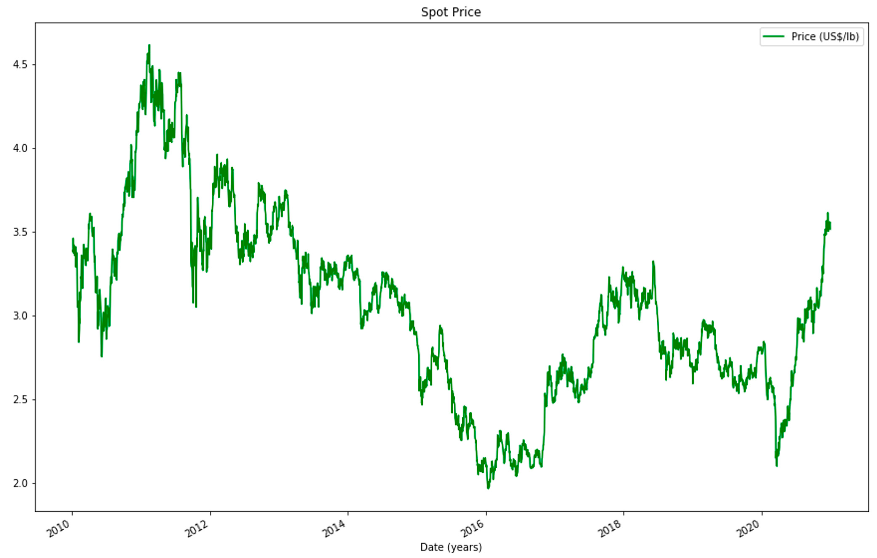
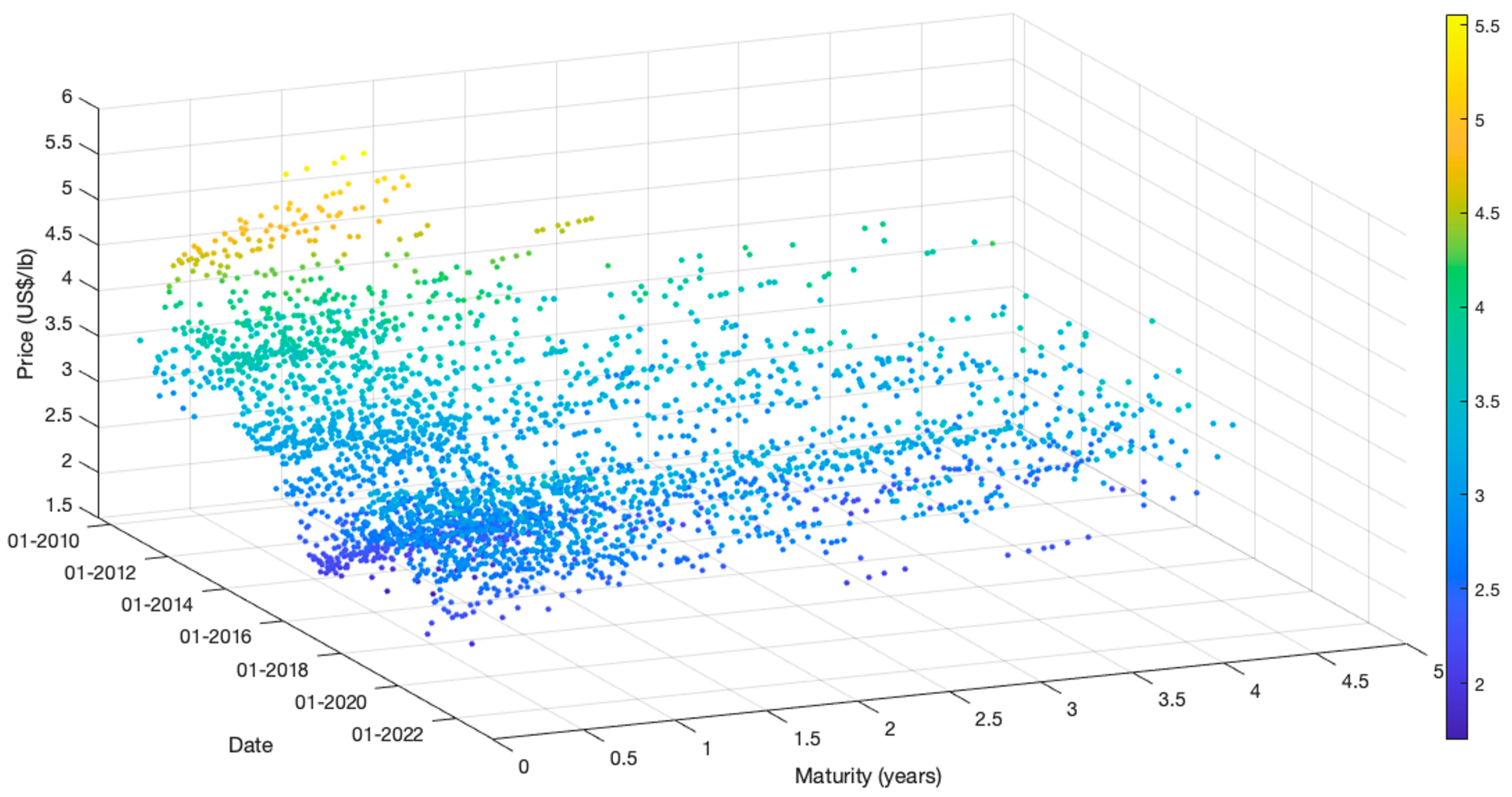
To illustrate the variability of these prices, Figure 1 plots them from January 2010 to December 2020.

4.2. Futures Prices

The two primary sources of copper futures prices are LME in the UK and COMEX in the USA. In the LME, futures expire in the current month and for the following 123 months. In the COMEX, futures expire in the current month, the next 23 months, and any March, May, July, September, and December within 60 months.

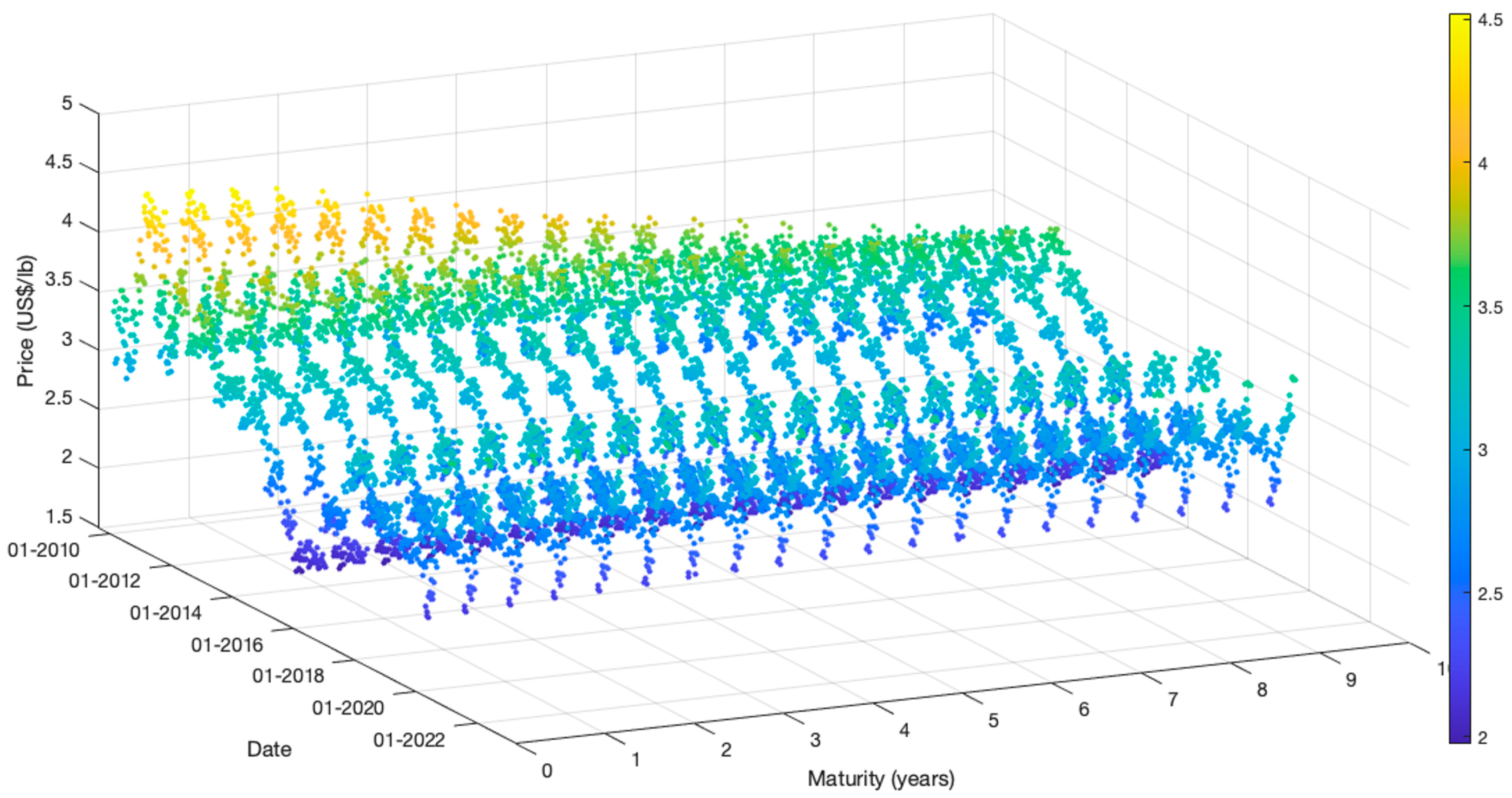
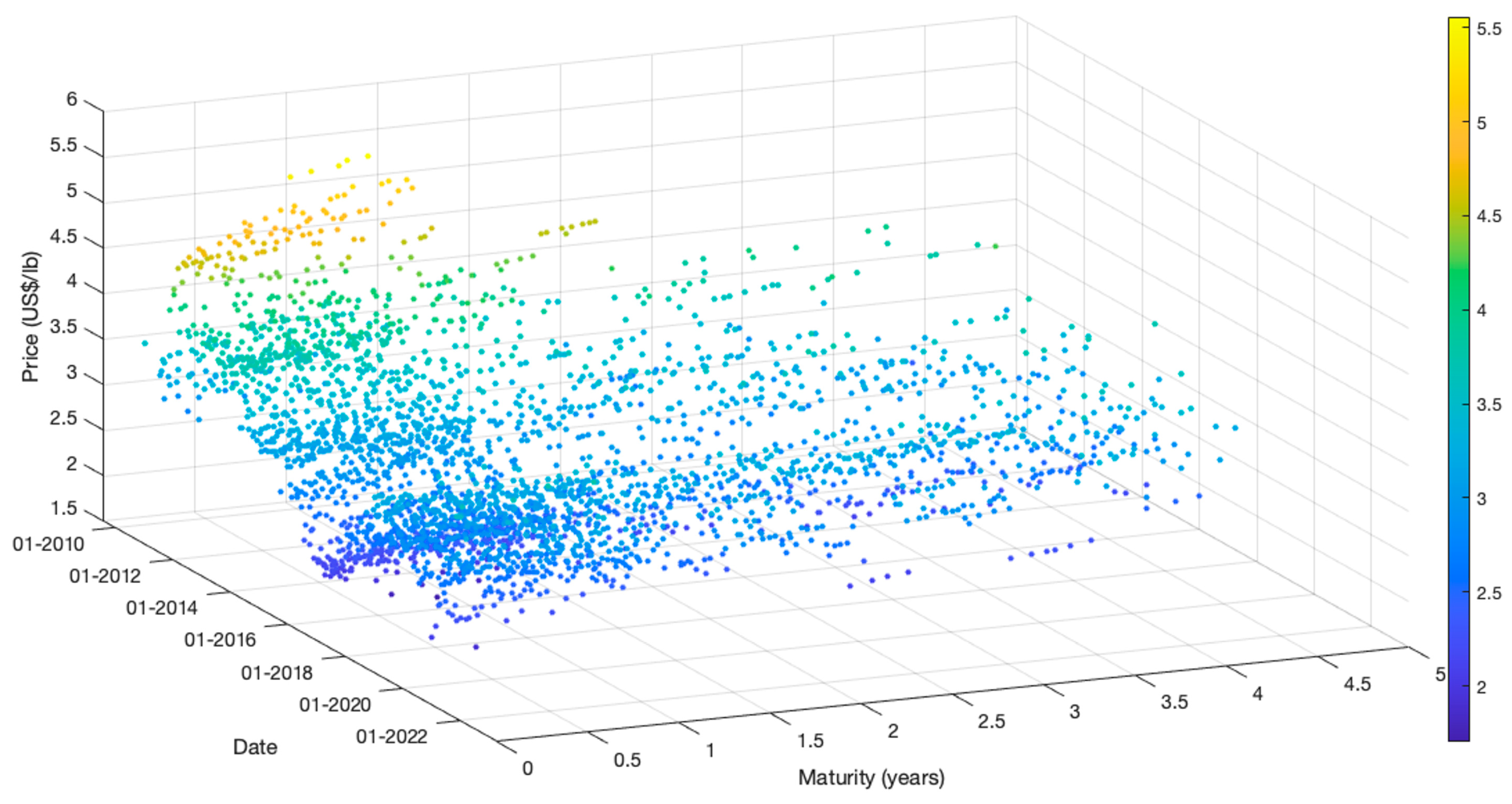
We will use futures prices for two purposes: first, as one of the inputs to the proposed model (joint futures and analysts’ expectations) described before. Following Cifuentes et al. (2020), we use LME weekly futures prices for the contract closest to its maturity and those maturing every six months. Figure 2 shows the LME weekly copper futures prices from January 2010 to December 2020, and

Table 1. LME weekly copper futures prices used as input to the model (in-sample), grouped by year.

Year	Amount of Data
2010	1040
2011	1040
2012	1040
2013	1040
2014	1060
2015	1040
2016	1040
2017	1040
2018	1040
2019	1040
Average	1042

summarizes the LME data used as input to the proposed model.

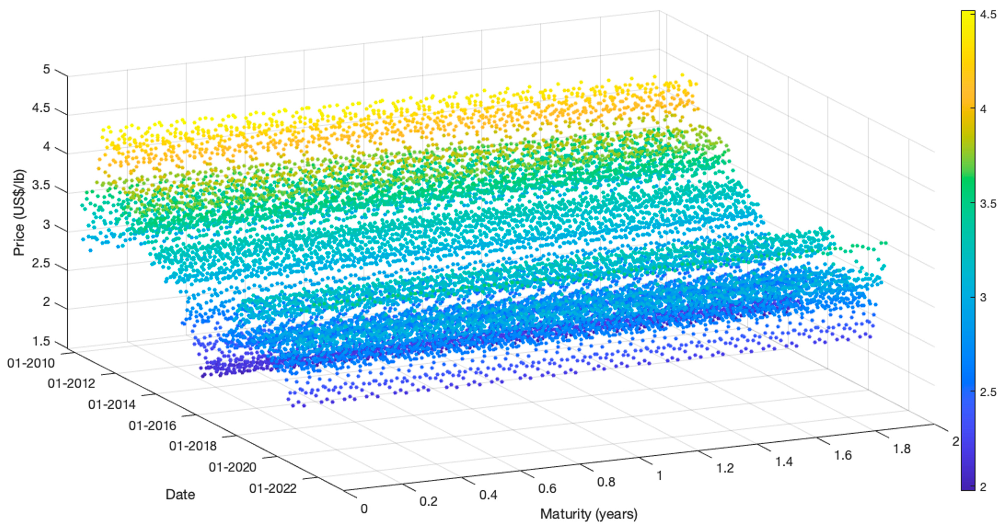
A second way of using futures data is as a forecast for the next 24 months of the spot prices. The following section compares forecasting performance using LME or COMEX futures contracts. The LME futures used as the spot price forecast include weekly data for contracts with maturities up to 24 months. Figure 3 and

Table 2. LME weekly futures prices up to 24 months (in-sample), grouped by year.

Year	Amount of Data
2010	1243
2011	1243
2012	1245
2013	1245
2014	1266
2015	1243
2016	1244
2017	1244
2018	1245
2019	1243
Average	1246.1

describe this data.

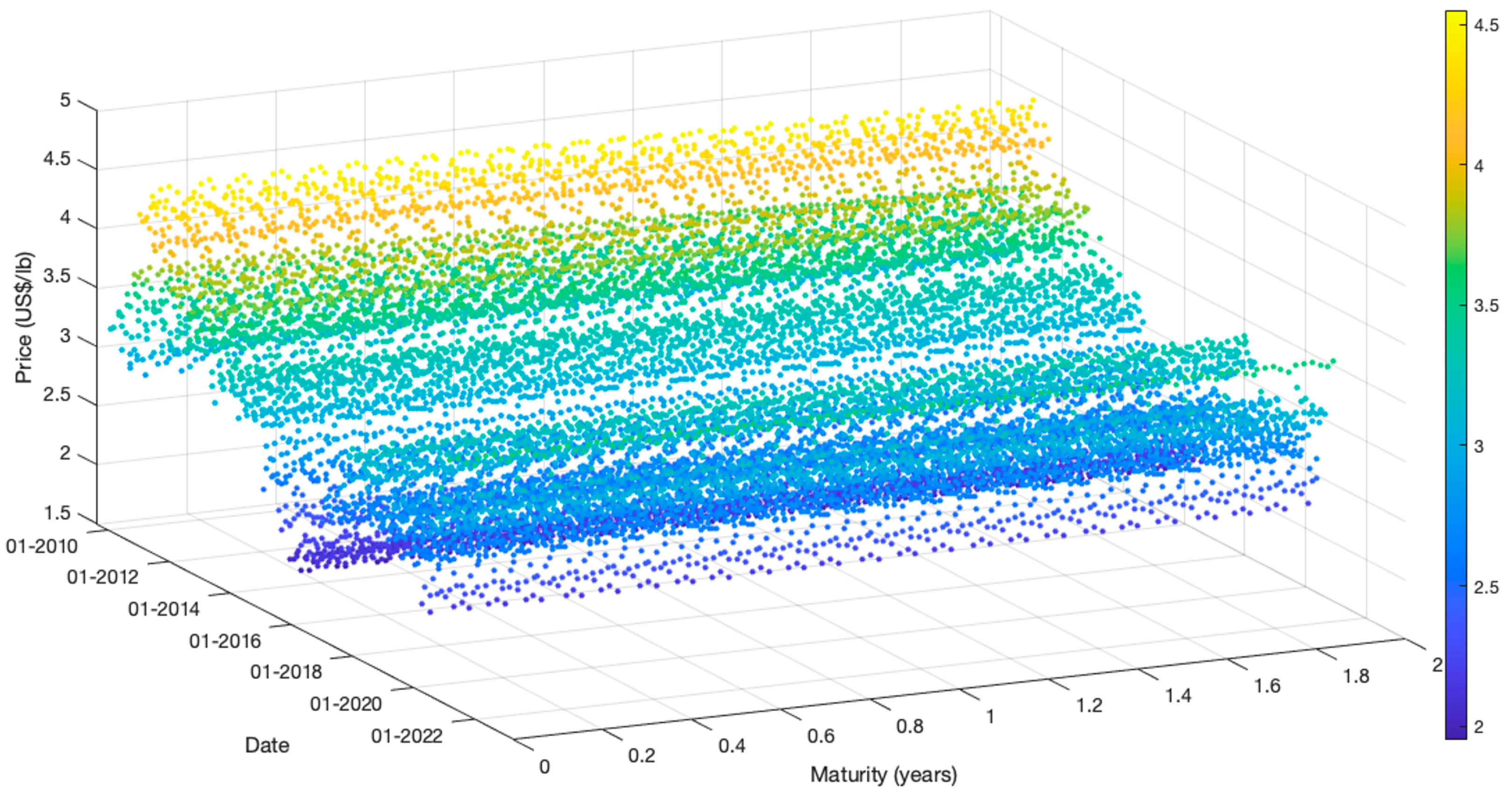
As mentioned, COMEX futures prices may also serve as spot price forecasts. Figure 4 and

Table 3. COMEX weekly futures prices up to 24 months (in-sample) by year.

Year	Amount of Data
2010	1250
2011	1249
2012	1236
2013	1231
2014	1258
2015	1248
2016	1251
2017	1251
2018	1273
2019	1286
Average	1253.3

present this data.

4.3. Analysts’ Consensus Expectations

Bloomberg reports forecasts from analysts at various financial institutions. There are two types of forecasts: quarterly and annual. These predictions are made for the average price each quarter or year. Following Cifuentes et al. (2020), they represent the price in the middle of their period.

Quarterly forecasts are available for the current quarter and for the following five quarters. Annual forecasts are valid for the year in which they are made and for the next 4 years. These forecasts are not available on a previously defined schedule. Analysts can forecast some, all, or none of these horizons at any given date. All forecasts in the same week and for the same horizon are averaged to obtain weekly analysts’ expectations data2.

Figure 5 shows all weekly analysts’ expectations data, while

Table 4. Analysts’ expectations up to 24 months (in-sample), grouped by year.

Year	Amount of Data
2010	240
2011	278
2012	344
2013	621
2014	711
2015	740
2016	783
2017	746
2018	561
2019	331
Average	535.5

summarizes analysts’ weekly expectations data for up to 24 months.

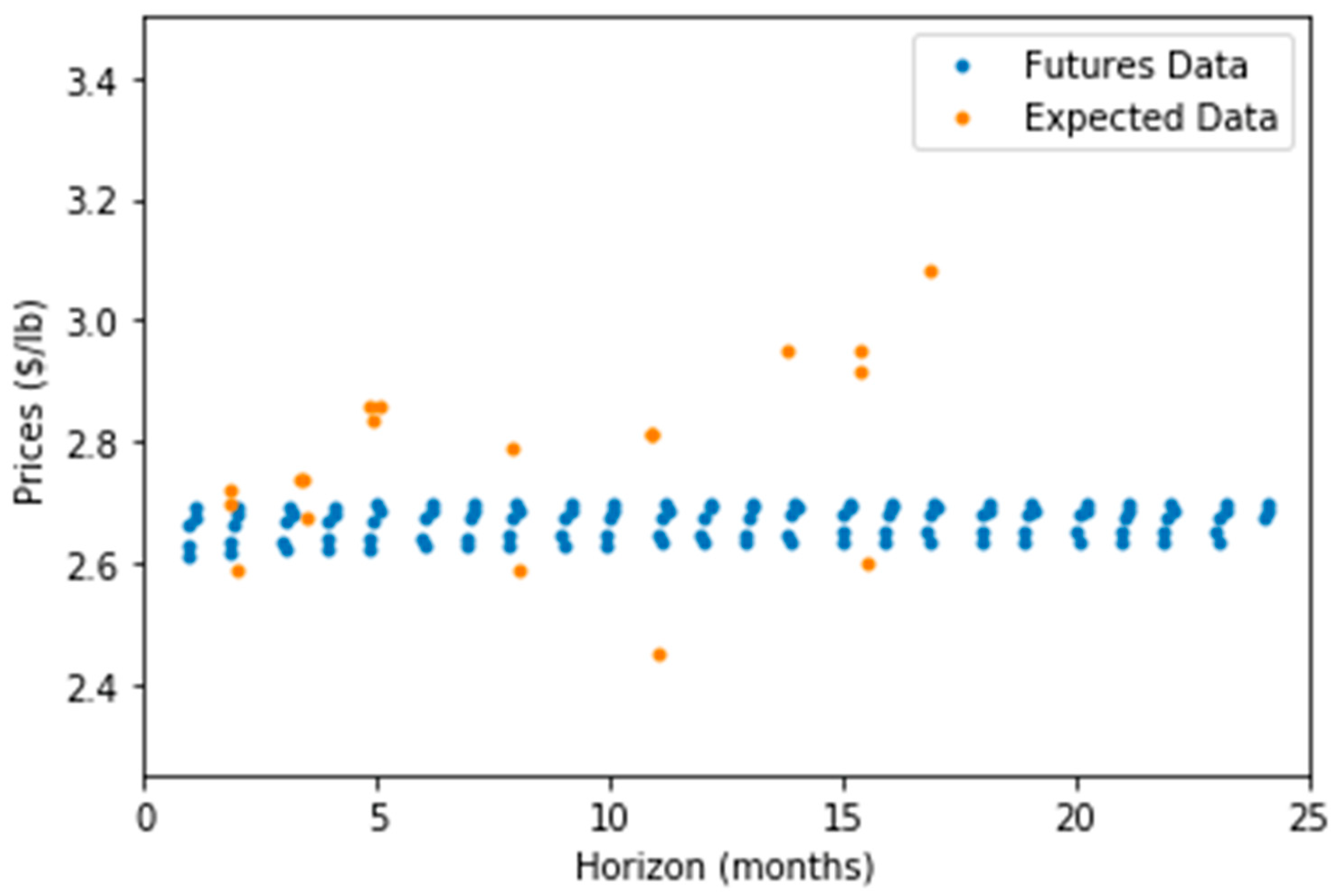
Given the variety of analysts, horizons, and dates, the data is particularly volatile and complex to use directly. Figure 6 shows how volatile the analysts’ data is during the week.

It becomes clear that to use this data effectively for forecasting, some smoothing is needed.

We are considering two ways of processing this data. The first one uses what Bloomberg reports as the consensus, the median of the available analyst forecasts for each horizon on a given week. Figure 7 and

Table 5. Bloomberg’s weekly consensus expectations (in-sample) by year.

Year	Amount of Data
2010	411
2011	460
2012	473
2013	490
2014	458
2015	453
2016	466
2017	425
2018	391
2019	407
Average	443.4

present this data.

The second way to smooth this volatile data is to apply the Kalman filter to all data shown in Figure 5 during calibration of our proposed model.

5. Forecasting Results

In what follows, we summarize the out-of-sample results applying the alternative forecasts to 1-to-24-month horizons from 2014 to 20203. Each result is ranked against the standard no-change forecast benchmark, with the best highlighted in bold.

5.1. Forecasting Results Using Futures

The forecast for any given horizon is calculated as the weighted average of the prices of the two futures with maturities closest to the horizon.

Table 6. RMSE performance metric using futures from 2014 to 2020, implemented with LME and COMEX. The “BEST” column shows the best model for each horizon.

Horizon (Months)	LME	COMEX	BEST
1	0.147	0.150	LME
3	0.262	0.265	LME
6	0.352	0.354	LME
9	0.407	0.410	LME
12	0.494	0.498	LME
15	0.551	0.557	LME
18	0.605	0.613	LME
21	0.642	0.651	LME
24	0.664	0.671	LME
Horizons up to 12 months	0.354	0.3577	LME
Horizons between 13 and 24 months	0.604	0.611	LME
Horizons up to 24 months	0.485	0.490	LME

The boldface indicates that the model performs better than the no-change benchmark.

,

Table 7. Relative MSPE performance metric using futures from 2014 to 2020 implemented with LME and COMEX. The “BEST” column shows the best model for each horizon.

Horizon (Months)	LME	COMEX	BEST
1	0.987	1.018	LME
3	0.978	0.997	LME
6	0.972	0.984	LME
9	0.965	0.975	LME
12	0.968	0.985	LME
15	0.971	0.992	LME
18	0.971	0.997	LME
21	0.983	1.009	LME
24	0.988	1.010	LME
Horizons up to 12 months	0.970	0.983	LME
Horizons between 13 and 24 months	0.976	1.000	LME
Horizons up to 24 months	0.974	0.995	LME

The boldface indicates that the model performs better than the no-change benchmark.

and

Table 8. Dstat performance metric using futures 2014–2020 implemented with LME and COMEX. The “BEST” column shows the best model for each horizon.

Horizon (Months)	LME	COMEX	BEST
1	0.587	0.507	LME
3	0.571	0.503	LME
6	0.644	0.559	LME
9	0.606	0.554	LME
12	0.589	0.510	LME
15	0.570	0.563	LME
18	0.564	0.610	COMEX
21	0.533	0.628	COMEX
24	0.544	0.659	COMEX
Horizons up to 12 months	0.599	0.526	LME
Horizons between 13 and 24 months	0.558	0.600	COMEX
Horizons up to 24 months	0.580	0.560	LME

The boldface indicates that the model performs better than the no-change benchmark.

present the RMSE, relative MSPE, and Dstat metrics using futures when implemented with LME or COMEX data.

Several conclusions may be obtained from the above tables. First, futures prices provide a better forecast for most metrics and horizons than the no-change benchmark. Second, LME futures give better forecasts than the no-change benchmark for all metrics and horizons. Lastly, LME futures provide better forecasts than COMEX futures for almost all horizons and performance metrics. This result is not surprising, given that the spot price to be forecasted is the cash price from LME.

If, for any reason, LME futures are not available, COMEX futures provide better forecasts than those of the no-change benchmark for some metrics, especially for horizons from 3 to 18 months.

5.2. Forecasting Results Using Analysts’ Consensus Expectations

As discussed, analysts’ expectations are very volatile, so some smoothing is required. In this section, we analyze performance using the consensus of analysts’ expectations, defined as the median of analysts’ predictions, as reported by Bloomberg.

The forecast for any given horizon is calculated as the weighted average of two analyst consensus forecasts closest to the horizon.

Table 9. Performance metrics using analysts’ consensus expectations from 2014 to 2020.

Horizon (Months)	RMSE	Relative MSPE	Dstat
1	0.230	2.392	0.565
3	0.321	1.466	0.545
6	0.409	1.317	0.462
9	0.477	1.322	0.450
12	0.553	1.215	0.494
15	0.600	1.151	0.533
18	0.623	1.031	0.592
21	0.642	0.981	0.620
24	0.611	0.839	0.663
Horizons up to 12 months	0.416	1.340	0.493
Horizons between 13 and 24 months	0.617	1.019	0.586
Horizons up to 24 months	0.518	1.113	0.536

The boldface indicates that the model performs better than the no-change benchmark.

shows that consensus forecasts are better than the no-change benchmark for all performance metrics for only 21- and 24-month horizons. The Dstat metric, which indicates whether prices are rising or falling, performs well, especially over longer horizons.

In summary, using analysts’ forecasts, as represented by Bloomberg’s consensus, yields mixed results, casting some doubt on the value of considering analysts’ expectations as a data source. This preliminary conclusion, however, will be revised in the next section.

5.3. Forecasting Results for the Model (Joint Futures and Analysts’ Expectations)

In this section, we explore the value of using analysts’ expectations alongside futures prices in a forecasting model calibrated using the Kalman filter.

5.3.1. Model Fit

The model must be calibrated several times to provide out-of-sample spot copper forecasts. The first dataset used to calibrate model parameters includes prices from 2010 to 2013, which are then used to forecast prices during 2014 for the next 24 months. Then, 1 year is added to the calibration dataset, parameters are estimated, and forecasts are generated for 2015. This process continues until the last dataset covers prices from 2010 to 2019, enabling forecasts for 2020. The model uses all available futures and analysts’ expectations data to estimate the expected and futures curves jointly.

Although no additional regularization techniques were applied, this rolling re-estimation procedure inherently mitigates overfitting, as model parameters are continuously updated and evaluated on out-of-sample data. The Kalman filter also contributes to this goal by smoothing transient shocks and reducing the influence of short-term noise in the estimation process.

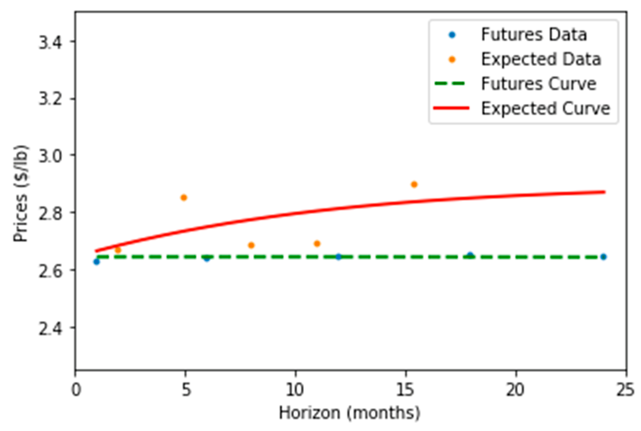
Figure 8 presents the expected and futures curves and data for the third week of March 2017. The expected curve does not perfectly fit the available data due to its volatility. However, the Kalman filter considers data from that week and all past data, providing a smooth expectation curve for each date. On the other hand, the futures curve fits the data much better because it is less volatile.

Table 10. Mean absolute percentage error of expected and futures curves (in-sample).

Calibration Years	MAPE (%) Between
	Curve and Futures Prices Data	Curve and Analysts’ Expected Prices Data
2010–2013	0.21%	6.77%
2010–2014	0.21%	6.62%
2010–2015	0.19%	6.59%
2010–2016	0.18%	6.71%
2010–2017	0.18%	6.86%
2010–2018	0.18%	6.88%
2010–2019	0.17%	6.85%
Average	0.19%	6.76%
Standard Deviation	0.01%	0.12%

and

Table 11. Mean absolute percentage error of expected and futures curves (out-of-sample). The “Year” column shows the out-of-sample year for each calibration year.

Calibration Years	Year	MAPE (%) Between
		Curve and Futures Prices Data	Curve and Analysts’ Expected Prices Data
2010–2013	2014	0.29%	5.36%
2010–2014	2015	0.36%	6.25%
2010–2015	2016	0.11%	11.51%
2010–2016	2017	0.18%	8.13%
2010–2017	2018	0.20%	5.67%
2010–2018	2019	0.11%	7.14%
2010–2019	2020	0.13%	5.10%
Average		0.19%	7.02%
Standard Deviation		0.10%	2.25%

compute the mean absolute percentage error (MAPE) for the in-sample and out-of-sample data. The futures curves fit better, as expected. Also, the average MAPE is similar between the in-sample and the out-of-sample calibrations.

5.3.2. Model Results

Table 12. Performance metrics for the model from 2014 to 2020.

Horizon (Months)	RMSE	Relative MSPE	Dstat
1	0.147	0.978	0.579
3	0.265	1.001	0.542
6	0.362	1.028	0.529
9	0.415	1.003	0.523
12	0.472	0.885	0.513
15	0.494	0.780	0.567
18	0.509	0.688	0.620
21	0.516	0.634	0.675
24	0.507	0.576	0.751
Horizons up to 12 months	0.356	0.981	0.537
Horizons between 13 and 24 months	0.505	0.684	0.629
Horizons up to 24 months	0.431	0.770	0.579

The boldface indicates that the model performs better than the no-change benchmark.

shows that using both futures and analysts’ expectations as inputs in the proposed model provides better forecasts than the no-change benchmark under all metrics for horizons of 1 month and 12 to 24 months. In addition, this holds for the Dstat metric for all horizons.

6. Comparing Forecasting Alternatives

In this section, we analyze the forecasting performance of the three alternatives using futures prices, consensus expectations, and the model. As a robustness check, we split the out-of-sample data into two parts.

Given that it is well known that, depending on market and inventory conditions, futures prices behave differently—sometimes in contango and sometimes in backwardation—we account for this when dividing the data. We must, however, consider that these two price regimes occur at different frequencies.

To generate the two files, we split the out-of-sample futures into high- and low-difference groups based on whether the difference between futures and spot prices is above or below the median of the corresponding in-sample data. Thus, the out-of-sample data is divided into two parts: when “futures are high”, which means that futures are in a relative contango, and when “futures are low” or in a relative backwardation.

6.1. Forecasting When “Futures Are High” (Relative Contango)

Table 13. RMSE for the model, LME, and consensus from 2014 to 2020 under high futures conditions. The “Best” column shows the best alternative for each horizon.

Horizon (Months)	Model	LME	Consensus	Best
1	0.153	0.154	0.231	Model
3	0.264	0.279	0.316	Model
6	0.364	0.388	0.428	Model
9	0.393	0.417	0.461	Model
12	0.420	0.472	0.507	Model
15	0.429	0.508	0.520	Model
18	0.396	0.529	0.479	Model
21	0.425	0.578	0.516	Model
24	0.429	0.613	0.486	Model
Horizons up to 12 months	0.345	0.370	0.411	Model
Horizons between 13 and 24 months	0.424	0.552	0.508	Model
Horizons up to 24 months	0.387	0.470	0.462	Model

The boldface indicates the best-performing alternative.

and

Table 14. Relative MSPE for the model, LME, and consensus from 2014 to 2020 under high futures. The “Best” column shows the best alternative for each horizon.

Horizon (Months)	Model	LME	Consensus	Best
1	0.983	0.989	2.237	Model
3	0.881	0.984	1.263	Model
6	0.862	0.982	1.191	Model
9	0.880	0.989	1.208	Model
12	0.789	0.997	1.148	Model
15	0.716	1.005	1.050	Model
18	0.565	1.011	0.831	Model
21	0.555	1.029	0.821	Model
24	0.506	1.032	0.650	Model
Horizons up to 12 months	0.858	0.988	1.218	Model
Horizons between 13 and 24 months	0.599	1.016	0.859	Model
Horizons up to 24 months	0.680	1.007	0.972	Model

The boldface indicates the best-performing alternative.

show that when futures prices are relatively high compared to spot prices (relative contango), the model performs much better than the alternatives across all horizons in terms of RMSE and relative MSPE. This shows that analysts’ expected prices, when used as inputs alongside futures prices, are valuable for forecasting.

On the other hand,

Table 15. Dstat for the model, LME, and consensus from 2014 to 2020 under high futures conditions. The “Best” column shows the best alternative for each horizon.

Horizon (Months)	Model	LME	Consensus	Best
1	0.576	0.587	0.565	LME
3	0.552	0.571	0.545	LME
6	0.593	0.644	0.462	LME
9	0.534	0.606	0.450	LME
12	0.495	0.589	0.494	LME
15	0.521	0.570	0.533	LME
18	0.582	0.564	0.592	Consensus
21	0.605	0.533	0.620	Consensus
24	0.696	0.544	0.663	Model
Horizons up to 12 months	0.549	0.599	0.493	LME
Horizons between 13 and 24 months	0.585	0.558	0.586	Consensus
Horizons up to 24 months	0.567	0.580	0.536	LME

The boldface indicates the best-performing alternative.

shows that for forecasting the direction of price movements, using detailed analysts’ expectations is not valuable. In this case, it is better to use LME futures prices for short-term horizons and consensus forecasts for long horizons.

6.2. Forecasting When “Futures Are Low” (Relative Backwardation)

Table 16. RMSE for the model, LME, and consensus from 2014 to 2020 under low futures conditions. The “Best” column shows the best alternative for each horizon.

Horizon (Months)	Model	LME	Consensus	Best
1	0.140	0.141	0.228	Model
3	0.267	0.241	0.327	LME
6	0.358	0.292	0.382	LME
9	0.444	0.394	0.499	LME
12	0.537	0.523	0.613	LME
15	0.586	0.615	0.714	Model
18	0.689	0.739	0.849	Model
21	0.691	0.778	0.877	Model
24	0.674	0.786	0.866	Model
Horizons up to 12 months	0.370	0.332	0.424	LME
Horizons between 13 and 24 months	0.642	0.698	0.797	Model
Horizons up to 24 months	0.494	0.507	0.597	Model

The boldface indicates the best-performing alternative.

,

Table 17. Relative MSPE for the model, LME, and consensus from 2014 to 2020 under low futures conditions. The “Best” column shows the best alternative for each horizon.

Horizon (Months)	Model	LME	Consensus	Best
1	0.972	0.984	2.583	Model
3	1.187	0.968	1.781	LME
6	1.428	0.948	1.622	LME
9	1.185	0.930	1.490	LME
12	0.989	0.937	1.287	LME
15	0.848	0.935	1.258	Model
18	0.808	0.931	1.227	Model
21	0.732	0.926	1.178	Model
24	0.680	0.923	1.120	Model
Horizons up to 12 months	1.170	0.941	1.531	LME
Horizons between 13 and 24 months	0.786	0.929	1.210	Model
Horizons up to 24 months	0.886	0.932	1.293	Model

The boldface indicates the best-performing alternative.

and

Table 18. Dstat for the model, LME, and consensus from 2014 to 2020 under low futures conditions. The “Best” column shows the best alternative for each horizon.

Horizon (Months)	Model	LME	Consensus	Best
1	0.582	0.587	0.565	LME
3	0.531	0.571	0.545	LME
6	0.440	0.644	0.462	LME
9	0.507	0.606	0.450	LME
12	0.538	0.589	0.494	LME
15	0.643	0.570	0.533	Model
18	0.699	0.564	0.592	Model
21	0.848	0.533	0.620	Model
24	0.900	0.544	0.663	Model
Horizons up to 12 months	0.522	0.599	0.493	LME
Horizons between 13 and 24 months	0.723	0.558	0.586	Model
Horizons up to 24 months	0.600	0.580	0.536	Model

The boldface indicates the best-performing alternative.

present the performance results of the three alternatives when the futures prices are relatively low compared to spot prices (relative backwardation). Results are very consistent across all three performance metrics, showing that, in this case, it is better to use LME futures prices for short-term horizons (up to 12 months) and the model for longer horizons.

7. Conclusions

Previous literature has argued that forecasting copper prices is relevant for many agents, including investors and governments. In this paper, we contribute to this issue even though research is still underway to find models and data sources that could be more useful in this endeavor.

This paper presents three alternatives for forecasting spot prices over horizons of 1 to 24 months. First, futures prices were used, and this alternative was implemented using either LME or COMEX futures. We concluded that, in this case, it was better to use LME futures.

Second, we considered analysts’ expectations and discussed how volatile this data is, noting the convenience of using a smoothing process. For this alternative, we initially used the consensus expectations reported by Bloomberg, which are the median of the available data for a given horizon.

The third alternative presented was to jointly consider futures and analysts’ expectations as input to a model that smooths data using the Kalman filter. All three options—futures, consensus, and model—were compared with the well-known no-change forecast benchmark and among themselves across different price scenarios.

The main conclusions that can be drawn from these exercises are the following. First, analysts’ expectations are a valuable source of data for forecasting copper prices. Second, since this data is very volatile, smoothing by using Bloomberg’s consensus data (which provides the median forecast) is not helpful. Third, when futures prices are relatively higher than spot prices (compared with recent history), the presented model is the best alternative for forecasting copper prices at any horizon between 1 and 24 months. Fourth, when prices are relatively lower than spot prices (compared with recent history), the model is the best alternative for long-term forecasts and the LME futures prices for 1 to 12 months.

Beyond these empirical results, forecasting copper prices has broader implications for investors, policymakers, and researchers. Investors can use copper prices as an early indicator of global economic performance, given copper’s importance across industries such as transportation, telecommunications, and construction. From a policy perspective, countries such as Chile and Zambia, whose fiscal revenues and overall economic performance are strongly dependent on copper exports, remain particularly exposed to price fluctuations. In these cases, improved forecasting accuracy can support the design of sovereign wealth fund management and macroeconomic stabilization mechanisms. Finally, from a theoretical standpoint, our findings contribute to the debate on the predictability of commodity prices.

While the results are encouraging, this study also has some limitations that should be acknowledged. The analysis is based on a specific time period and relies on weekly data from LME, COMEX, and Bloomberg, which may not fully capture the underlying dynamics of commodity markets. Future research could extend this framework by incorporating additional macro-financial variables or by exploring the predictive relationships between copper and other commodities. Further work could also examine how improved price forecasts translate into more effective investment strategies and fiscal policies in resource-dependent economies.

References

- Alameer, Zakaria, Mohamed Abd Elaziz, Ahmed A. Ewees, Haiwang Ye, and Zhang Jianhua. 2019. Forecasting Copper Prices Using Hybrid Adaptive Neuro-Fuzzy Inference System and Genetic Algorithms. Natural Resources Research 28: 1385–401. [Google Scholar] [CrossRef]
- Alquist, Ron, Lutz Kilian, and Robert J. Vigfusson. 2013. Forecasting the price of oil. In Handbook of Economic Forecasting. Amsterdam: Elsevier B.V., vol. 2. [Google Scholar] [CrossRef]
- Boyd, Naomi E., Jeffrey H. Harris, and Bingxin Li. 2018. An update on speculation and financialization in commodity markets. Journal of Commodity Markets 10: 91–104. [Google Scholar] [CrossRef]
- Buncic, Daniel, and Carlo Moretto. 2015. Forecasting copper prices with dynamic averaging and selection models. North American Journal of Economics and Finance 33: 1–38. [Google Scholar] [CrossRef]
- Chen, Yanhui, Kaijian He, and Chuan Zhang. 2016. A novel grey wave forecasting method for predicting metal prices. Resources Policy 49: 323–31. [Google Scholar] [CrossRef]
- Cifuentes, Sebastián, Gonzalo Cortazar, Hector Ortega, and Eduardo S. Schwartz. 2020. Expected prices, futures prices and time-varying risk premiums: The case of copper. Resources Policy 69: 101825. [Google Scholar] [CrossRef]
- Ciner, Cetin, Brian Lucey, and Larisa Yarovaya. 2020. Spillovers, integration and causality in LME non-ferrous metal markets. Journal of Commodity Markets 17: 100079. [Google Scholar] [CrossRef]
- Cortazar, Gonzalo, Hector Ortega, and Consuelo Valencia. 2021. How good are analyst forecasts of oil prices? Energy Economics 102: 105500. [Google Scholar] [CrossRef]
- Cortazar, Gonzalo, Hector Ortega, and José Antonio Pérez. 2025. Using Futures Prices and Analysts’ Forecasts to Estimate Agricultural Commodity Risk Premiums. Risks 13: 9. [Google Scholar] [CrossRef]
- Cortazar, Gonzalo, Hector Ortega, Joaquin Santa Maria, and Eduardo S. Schwartz. 2024. Expected returns on commodity ETFs and their underlying assets. Journal of Commodity Markets 36: 100469. [Google Scholar] [CrossRef]
- Cortazar, Gonzalo, Ivo Kovacevic, and Eduardo S. Schwartz. 2015. Expected commodity returns and pricing models. Energy Economics 49: 60–71. [Google Scholar] [CrossRef]
- Cortazar, Gonzalo, Philip Liedtke, Hector Ortega, and Eduardo S. Schwartz. 2022. Time-Varying Term Structure of Oil Risk Premiums. The Energy Journal 43: 71–92. [Google Scholar] [CrossRef]
- Dehghani, Hesam. 2018. Forecasting copper price using gene expression programming. Journal of Mining and Environment 9: 349–60. [Google Scholar] [CrossRef]
- Dehghani, Hesam, and Dejan Bogdanovic. 2018. Copper price estimation using bat algorithm. Resources Policy 55: 55–61. [Google Scholar] [CrossRef]
- Dooley, Gillian, and Helena Lenihan. 2005. An assessment of time series methods in metal price forecasting. Resources Policy 30: 208–17. [Google Scholar] [CrossRef]
- García, Diego, and Werner Kristjanpoller. 2019. An adaptive forecasting approach for copper price volatility through hybrid and non-hybrid models. Applied Soft Computing Journal 74: 466–78. [Google Scholar] [CrossRef]
- Kalman Rudolph Emil. 1960. A new approach to linear filtering and prediction problems. Journal of Basic Engineering 82: 35–45. [Google Scholar] [CrossRef]
- Kriechbaumer, Thomas, Andrew Angus, David Parsons, and Monica Rivas Casado. 2014. An improved wavelet-ARIMA approach for forecasting metal prices. Resources Policy 39: 32–41. [Google Scholar] [CrossRef]
- Li, Gang, and Yong Li. 2015. Forecasting copper futures volatility under model uncertainty. Resources Policy 46: 167–76. [Google Scholar] [CrossRef]
- Liu, Chang, Zhenhua Hu, Yan Li, and Shaojun Liu. 2017. Forecasting copper prices by decision tree learning. Resources Policy 52: 427–34. [Google Scholar] [CrossRef]
- Sánchez Lasheras, Fernando, Francisco Javier de Cos Juez, Ana Suárez Sánchez, Alicja Krzemień, and Pedro Riesgo Fernández. 2015. Forecasting the COMEX copper spot price by means of neural networks and ARIMA models. Resources Policy 45: 37–43. [Google Scholar] [CrossRef]
- Stock, James H., and Mark W. Watson. 2004. Combination forecasts of output growth in a seven-country data set. Journal of Forecasting 23: 405–30. [Google Scholar] [CrossRef]
- Tang, Ke, and Wei Xiong. 2012. Index investment and the financialization of commodities. Financial Analysts Journal 68: 54–74. [Google Scholar] [CrossRef]
- Wang, Chao, Xinyi Zhang, Minggang Wang, Ming K. Lim, and Pezhman Ghadimi. 2019. Predictive analytics of the copper spot price by utilizing complex network and artificial neural network techniques. Resources Policy 63: 101414. [Google Scholar] [CrossRef]
- Watkins, Clinton, and Michael McAleer. 2004. Non-Ferrous Metal Prices. Journal of Economic Surveys 18: 651–702. [Google Scholar] [CrossRef]
- Wets, Roger J. B., and Ignacio Rios. 2015. Modeling and estimating commodity prices: Copper prices. Mathematics and Financial Economics 9: 247–70. [Google Scholar] [CrossRef]
- Yao, Jingtao, and Chew Lim Tan. 2000. A case study on using neural networks to perform technical forecasting of forex. Neurocomputing 34: 79–98. [Google Scholar] [CrossRef]
Figure 1.
Copper spot prices from January 2010 to December 2020.
Figure 2.
LME weekly copper futures prices from January 2010 to December 2020.
Figure 3.
LME weekly copper futures prices from January 2010 to December 2020 (2-year horizon).
Figure 4.
COMEX weekly copper futures prices from January 2010 to December 2020 (2-year horizon).
Figure 5.
Weekly data of analysts’ expectations from January 2010 to December 2020.
Figure 6.
Futures and analysts’ expected price data, third week, March 2017.
Figure 7.
Bloomberg’s weekly consensus expectations.
Figure 8.
Expected and futures curves and data, third week, March 2017.