Article

Multi-Timescale Recurrent Neural Networks Beat Rough Volatility for Intraday Volatility Prediction

Université Paris-Saclay, CentraleSupélec, Laboratoire MICS, 91190 Gif-sur-Yvette, France
*
Author to whom correspondence should be addressed.
Risks 2024, 12(6), 84; https://doi.org/10.3390/risks12060084
Submission received: 19 April 2024 / Revised: 16 May 2024 / Accepted: 20 May 2024 / Published: 22 May 2024
(This article belongs to the Special Issue Advances in Volatility Modeling and Risk in Markets)

Abstract

:
We extend recurrent neural networks to include several flexible timescales for each dimension of their output, which mechanically improves their abilities to account for processes with long memory or highly disparate timescales. We compare the ability of vanilla and extended long short-term memory networks (LSTMs) to predict the intraday volatility of a collection of equity indices known to have a long memory. Generally, the number of epochs needed to train the extended LSTMs is divided by about two, while the variation in validation and test losses among models with the same hyperparameters is much smaller. We also show that the single model with the smallest validation loss systemically outperforms rough volatility predictions for the average intraday volatility of equity indices by about 20% when trained and tested on a dataset with multiple time series.

1. Introduction

Some time series in nature have a very long memory (Robinson 2003), e.g., fluid turbulence (Resagk et al. 2006), asset price volatility (Cont 2001) and tick-by-tick events in financial markets (Challet and Stinchcombe 2001; Lillo and Farmer 2004). From a modelling point of view, this means that the current value of an observable of interest depends on the past by a convolution of itself with a long-tailed kernel.
Deep learning tackles past dependence in time series with recurrent neural networks (RNNs). These networks are in essence moving averages of nonlinear functions of the inputs and learn the parameters of these averages and functions. Provided that they are sufficiently large, these networks can approximate long-tailed kernels in a satisfactory way, and are of course able to account for more complex problems than a simple linear convolution. Yet, their flexibility may prevent them from learning the long memory of time series quickly and efficiently. Several solutions exist: either one pre-filters the data by computing statistics at various timescales and use them as inputs to RNNs in the same spirit as multi-timescale volatility modelling (Corsi 2009; Zumbach and Lynch 2001), see, e.g., Kim and Won (2018) or Ganesh and Rakheja (2018), or one extends the neural networks so as to improve their abilities. For example, Zhao et al. (2020) add delay operators, taking inspiration from ARIMA processes, to the states of recurrent neural networks, while Ohno and Kumagai (2021) modify the update equation of the network output so that its dynamics mimic those of a variable with a long memory. In both cases, the time dependence structure is enforced by hand in the architecture of neural networks or in the data that are input to the networks.
Here, we propose a flexible and parsimonious way to extend the long-memory abilities of recurrent neural networks by using an old trick: approximating long-memory kernels with exponential functions, which helps recurrent neural networks learn faster and better to predict time series with long memory.
Our main contributions are (i) we introduce RNNs with several multiple flexible timescales for each dimension of the output; (ii) we show that learning to predict time series with a long memory (asset price volatility) is faster and more reliable with more flexible timescales; and (iii) vanilla rough volatility predictions can be beaten by training a fair number of recurrent neural networks on multiple time series and only using the one with the best validation loss.

2. Materials and Methods

2.1. Recurrent Neural Networks with Multiple Timescales

Let time series y t be of interest. Its moving average can be written as
y ˜ t = t K ( t t ) y t d t ,
where K is a kernel. In a discrete-time context,
y ˜ t = t K ( t t ) y t .
When the process is Markovian, its kernel is K ( x ) e x / τ 0 for large x, where τ 0 is the slowest timescale at which the process forgets its past. In this case, one can write y t in a recursive way:
y ˜ t = y ˜ t 1 ( 1 λ ) + λ y t ,
where λ 1 / τ 0 ; y ˜ t is then an exponentially moving average (EMA) of y t .
Long memory processes, however, have a kernel that decreases at least as slowly as a power law with an exponent smaller than one (Palma 2007). In turn, power laws can be approximated by a sum of exponential functions; naively, if K ( z ) = z α , one writes
K ( z ) i = 1 w i exp ( z / τ i )
with w i ( 1 / c α ) i and τ i = c i for a well-chosen constant c. One covers the z space in a geometric way and the weights w i account for the power-law decreasing nature of K ( z ) . This rough approach works well and is widespread. Bochud and Challet (2007) propose a more refined method to determine how many exponential functions one needs to optimally approximate K and how to compute w i for a given α and for a given range of z over which the kernel has to be approximated by a sum of exponential functions. For example, one needs about four exponential functions to approximate a given power-law over three decades (e.g., z [ 1 , 1000 ] ).
Writing down the update equations of well-known recurrent neural network architectures makes it clear that they use exponentially moving averages with a single timescale for each output dimension. For example, gate recurrent units (GRUs) (Cho et al. 2014) transform the input vector x t R N I into a vector of timescales λ t R N O
λ t = σ ( W λ x t + U λ c t 1 + b λ ) ,
which is then used in the update of the output c t
c t = c t 1 ( 1 λ t ) + λ t c ˜ t ,
where the update c ˜ t is also computed from the input with learned weights, i.e.,
c ˜ t = σ c ( W c x t + U c ( c t 1 r t ) + b c )
r t = σ r ( W r x t + U r c t 1 + b r )
For non-linear functions σ c and σ r , ⊙ is the element-wise (Hadamar) product and r t is the reset gate which modifies the value of c t 1 when computing c ˜ t . By design, GRUs can only exponentially compute moving averages of c ˜ t (which itself is then modified non-linearly), although they possess the interesting ability to learn both λ t and the update c ˜ t as a function of their inputs. It is straightforward to extend GRUs to an arbitrary number of timescales n by using n  c ˜ t ( k ) , k = 1 , , n and
λ t ( k ) = σ ( W λ ( k ) x t + U λ ( k ) c t 1 ( k ) + b λ ( k ) )
c t ( k ) = c t 1 ( k ) ( 1 λ t ( k ) ) + λ t ( k ) c ˜ t ,
where each c t ( k ) is an exponentially moving average at a timescale proportional to 1 / λ t ( k ) . Finally, the output will be
c t = k = 1 n w k c t ( k ) ,
The simple α -RNNs (Dixon and London 2021), which are simplified GRUs, share the same assumption of a single timescale per output dimension and thus can be generalized in the same way. Let us show now how to extend LSTMs with a forget gate (Gers et al. 2000). Starting from their output h t R N h , one has
h t = o t σ h ( c t )
c t = f t c t 1 + i t c ˜ t ,
where o t , i t , and c ˜ t are determined from the input x t and the previous output h t 1 with learned weights, and σ h is a nonlinear function. Writing f t = 1 λ t makes it obvious that the cell vector c t evolves in the same way as y t in Equation (6) if i t λ t .
Extending LSTMs to include n timescales by cell state dimension is therefore straightforward: one needs to compute n EMAs and their associated timescales as follows:
f t ( k ) = σ ( W f ( k ) x t + U f ( k ) h t 1 + b f ( k ) )
i t ( k ) = σ ( W i ( k ) x t + U i ( k ) h t 1 + b i ( k ) )
c t ( k ) = f t ( k ) c t 1 ( k ) + i t ( k ) c ˜ t ,
where c ˜ t follows Equation (7), in which c t 1 evolves according to Equation (11). Note that one could set i t ( k ) = 1 f t ( k ) = λ t ( k ) and not learn the weights associated with i t . Learning i ( k ) as well is equivalent to modulating the importance of the update, which is known as cognitive bias (Palminteri et al. 2017); this is made clear by writing i t ( k ) = v t ( k ) ( 1 f t ( k ) ) = v t ( k ) λ t ( k ) , where v t ( k ) is the modulation of the learning speed.
We will focus on the case n = 2 ; after setting w 2 = ( 1 w 1 ) , (11) amounts to
c t = c t ( 1 ) w 1 + ( 1 w 1 ) c t ( 2 ) ,
where the vector w 1 is learnable and its components are bounded to the [ 0 , 1 ] interval. We call LSTMs with several timescales ( n > 1 ) per dimension LaSTMs, which stands for long and short-term memories (at the same time in a given hidden dimension). We reiterate that this architecture is introduced in order to significantly increase the memory length of a hidden dimension while not doubling the number of parameters. Other approaches, such as VLSTMs (Ganesh and Rakheja 2018), are orthogonal to ours, as they train an LSTM for each data resampling frequency. Here, we keep the complexity to a minimum while retaining the full flexibility of LSTMs; i.e., we do not impose a data resampling frequency by hand.
Naively, when learning to predict a process that is not too noisy, we expect the difference between LaSTM and LSTM to be the highest when N h = 1 , i.e., precisely when LSTMs are not able to compute long-term averages, and to decrease when N h increases.
Note that LSTMs with a sufficiently large cell dimension N h can in principle learn to superpose timescales in the same way as Equation (11) by learning one timescale per dimension and using a final dense layer to learn how to combine them (effectively learning the w 1 vector). However, imposing constraints (or equivalently, injecting some known structure) is known to lead to faster learning and better results (e.g., physics-guided deep learning; see Thuerey et al. (2021) for a review). This makes LSTM training less of a hit-and-miss process, as we shall see. We also emphasize that LaSTMs have fully flexible timescales and hence learn fully flexible averaging kernels.
We do not intend to provide here a comprehensive study of the best possible volatility prediction technique with deep learning involving more complex architectures, e.g., stacked LSTMs, LSTM with CNNs, VLSTMs, LSTMS with attention, etc. Instead, we focus on how to make vanilla LSTMs converge better and faster, which will mechanically improve all the above variations; we first investigate how long memory is better learned with several timescales per hidden state. A second research question is how to use a collection of trained LSTMs: we advocate to use the one with the smallest validation loss instead of taking averages. A final question is that of the universality of the volatility process, i.e., the ability of a model to predict the volatility of many time series, which we confirm here.

2.2. Volatility Prediction

Given an asset price P t and its log return r t = log P t log P t 1 , the asset price volatility σ is defined as σ = E ( r 2 ) . The dynamics of financial markets are ever-changing, which results in a temporal dependence of σ with clear patterns of long-term dependence (Cont 2001).
Risk management, portfolio optimization, and option pricing benefit from the ability to predict the evolution of σ t . Fortunately, σ t is relatively easy to predict owing to its long memory (Cont 2001); for example, its auto-correlation decreases very slowly, presumably as a power-law over more than a year. Econometric models include GARCH, whose simplest version involves only one timescale, while many variations use several timescales (Corsi 2009; Zumbach 2015; Zumbach and Lynch 2001). Rough volatility (Gatheral et al. 2018), on the other hand, considers log σ t as fractional Brownian motion and thus includes all timescales. As can be expected, rough volatility models outperform GARCH-based models for volatility prediction. Using LSTMs for volatility prediction is demonstrated, e.g., in Filipović and Khalilzadeh (2021); Ganesh and Rakheja (2018); Kim and Won (2018); Rosenbaum and Zhang (2022), which use various types of predictors (including GARCH models) and architectures. Notably, Rosenbaum and Zhang (2022) show that the average predictions of 10 stacked LSTMs with the past volatility and price return as predictors match the performance of rough volatility and has universality properties; i.e., a single model is able to predict the volatility dynamics of many assets.

2.3. Architecture and Hyperparameters

Our first aim is to characterize the effects of multiple timescales per cell dimension. Therefore, we compare simple non-stacked LSTMs with or without the proposed modification. Stacked LSTMs can learn additional timescales at the cost of doubling the number of parameters, which we precisely wish to avoid here. We pass the outputs h t of the LSTMs and LaSTMs through a dense layer of size N h with sigmoid activation functions, to combine the outputs in a non-trivial way, and a final dense layer with a single neuron with linear activation that converts the output of the LaSTMs into an estimate of the volatility. Both final layers have a bias term, which allows the model to learn a baseline volatility level. The loss is the MSE of the log volatility. In other words, we ask the artificial neural networks to minimize the relative prediction error instead of the absolute one. This choice is also more robust as it accounts for the large range of values for volatility and decreases the influence of rare and large events on the MSE.
We report a systematic study of the relative performance of LSTMs vs. LaSTMs. We vary the sequence length T seq from 10 to 100 by steps of 15, and the dimension of the hidden state is N h { 1 , , 5 } . Finally, we train models with and without biases (except for the final two dense layers which always have biases). There are thus 70 variations of hyperparameters per architecture choice.
For each hyperparameter and architecture couple, we train 20 networks, which yields 2800 models altogether. We use a standard 60/20/20 train/validation/test split and apply an early stopping criterion of the minimum validation loss over the five last epochs, with a maximum of 1000 epochs. The batch size is set to 128. Computations were carried out on a large CPU cluster using Tensorflow 2.12. We train the networks to predict log σ t + 1 with an MSE loss function.
We use the following data workflow: all the data used in this paper come from a dataset published by the Oxford-Man Institute, which contains daily index prices and estimates of intraday realized volatility for 31 indices1 and 2117 to 5385 data points per index (Heber et al. 2022). From this dataset, we keep the rk_twoscale column that corresponds to the two-scale realized kernel estimation method (Barndorff-Nielsen et al. 2008) and compute Close-to-Close returns. The predictors are then the log volatility itself and lagged Close-to-Close returns, as in Rosenbaum and Zhang (2022). Since the volatility individual time series start and end on heterogeneous dates, we used the dates to define the train/validation/test splits: the train set ranges from 4 January 2000 to 6 September 2012, the validation set from 7 September 2012 to 23 November 2016 and the test set from 24 November 2016 to 17 February 2021. This is necessary as the time series are cross-correlated; hence, splitting them according to their respective length would cause information leakage from the future and thus overfitting.

3. Results

3.1. Average Loss

Let us plot the average test loss of LSTMs and LaSTMs as a function of N h at fixed T seq , the dimension of the memory cell, and T s e q at fixed N h . This approach is taken by Rosenbaum and Zhang (2022), who trained 10 LSTMs instead of 20 here. Figure 1 shows that LaSTMs enjoy a sizeable advantage on average. We note that when N h = 1 , our initial intuition was correct: LaSTMs have a smaller average test loss for all variations of hyperparameters ( T seq and bias).
Large loss fluctuations among models are associated with large average test losses for both LaSTMs and LSTMs; however, the test losses of LaSTMs are more likely to be small (and have accordingly small fluctuations). This is explained by the large difference in training convergence time, as shown below. We also note that, at least for volatility prediction, keeping bias terms in the computation of i, f, c ˜ , and c (referred to as internal biases henceforth) is manifestly problematic; it turns out to be the default option both for PyTorch and Keras and is probably implicitly used in other papers. On the whole, we note that a simple average of the outputs of an ensemble of models leads to quite large fluctuations; hence, the question of the convergence of the models must be investigated, and a way to select good models would vastly improve the usefulness of LSTMs in this context.
Convergence during the training process, it turns out, is a hit and miss process: some models are stuck in a high-loss regime, while some models do learn a more realistic dynamical process and achieve much lower losses. This yields a bi-modal density of losses (see Figure 2). It is noteworthy that the fraction of LaSTMs that learn better is much larger. This is linked to the fact that LaSTMs learn much faster (see below) and that LaSTMs without internal biases are less likely to be stuck in a high loss regime.
We take the simple rough volatility model as our first benchmark (Gatheral et al. 2018): the vanilla rough volatility model assumes that log σ t follows a fractional Brownian motion; given a time series, there are only a few parameters to calibrate and predictions are obtained from a formula (see Gatheral 2016).
The very fact that even this simple rough volatility model is able to predict volatility relatively well strongly suggests that the test loss of any well-trained model should be commensurate with the validation loss, itself commensurate with the train loss. This is exactly what happens for neural networks as well, as shown in Figure 2. The same figure also shows that test losses are bimodal as well, with the majority of models not stuck in the high loss regime and some having a test loss substantially smaller than vanilla rough volatility models.
The vanilla rough volatility model can be extended to account for the Zumbach effect (Zumbach 2010), which reflects the influence of recent trends on future volatility, as in (Rosenbaum and Zhang 2021). Other simpler volatility models, such as that of Guyon and Lekeufack (2023), also contain a Zumbach term. Whereas this term significantly improves the implied volatility prediction in both models, we did not find any improvement in average intraday volatility prediction with respect to vanilla rough volatility, and hence we only report the results for the latter.

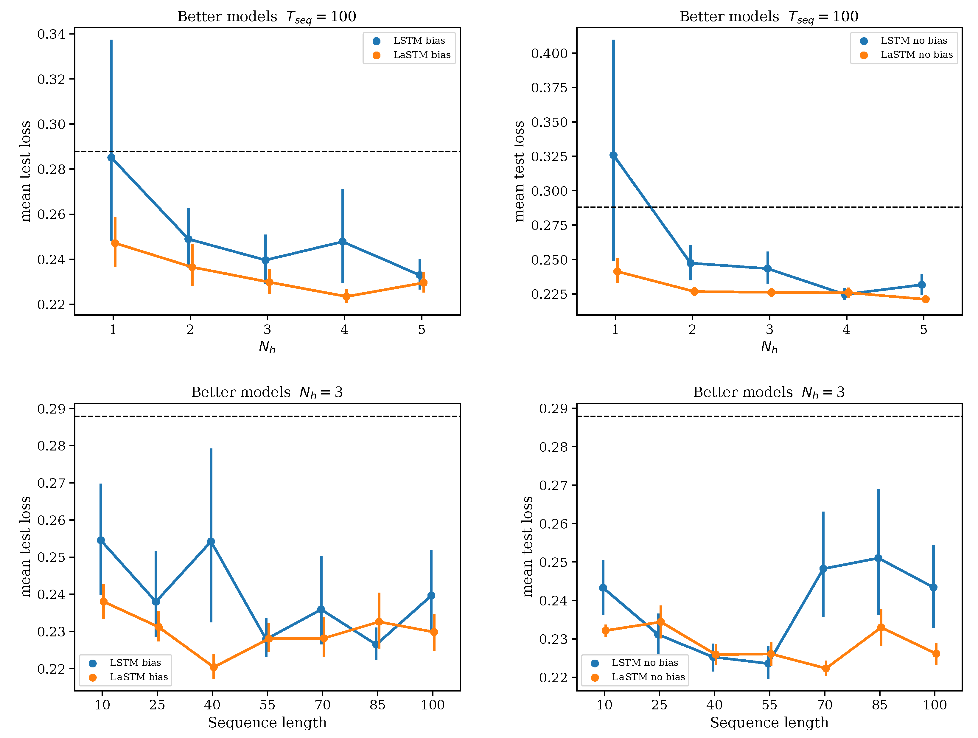
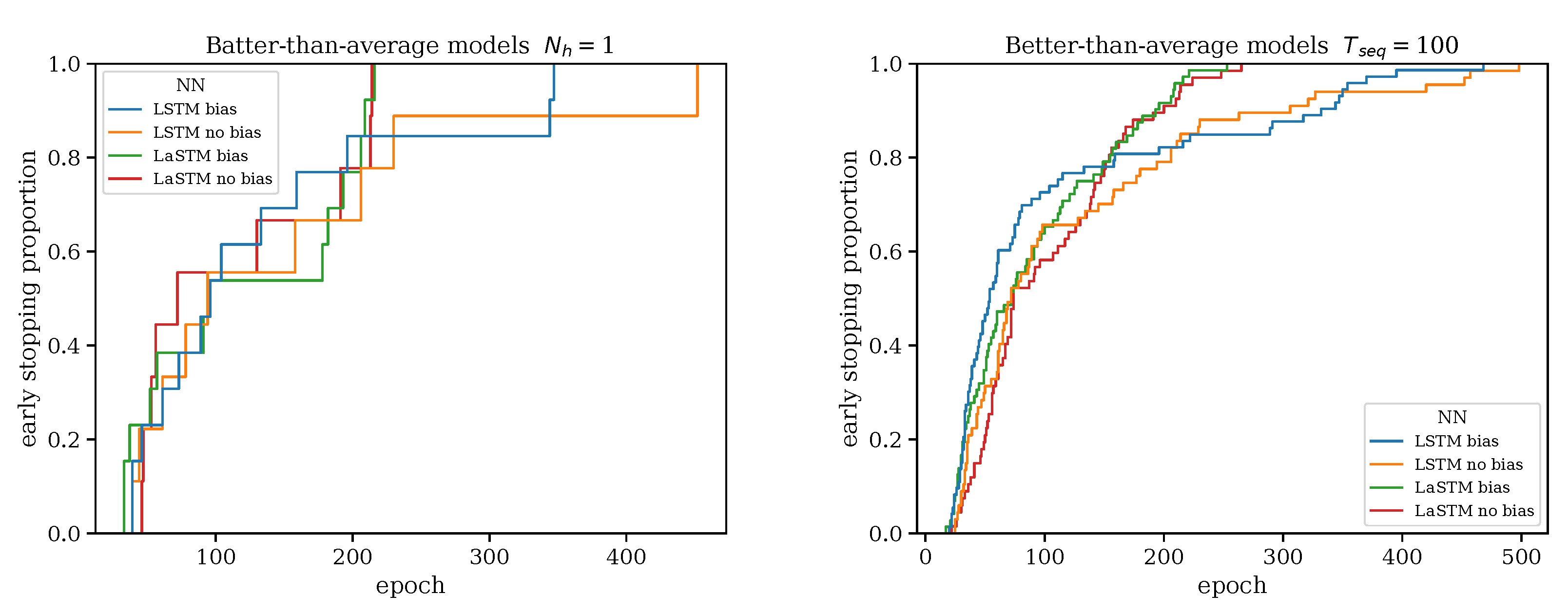
3.2. Keeping the Better Models
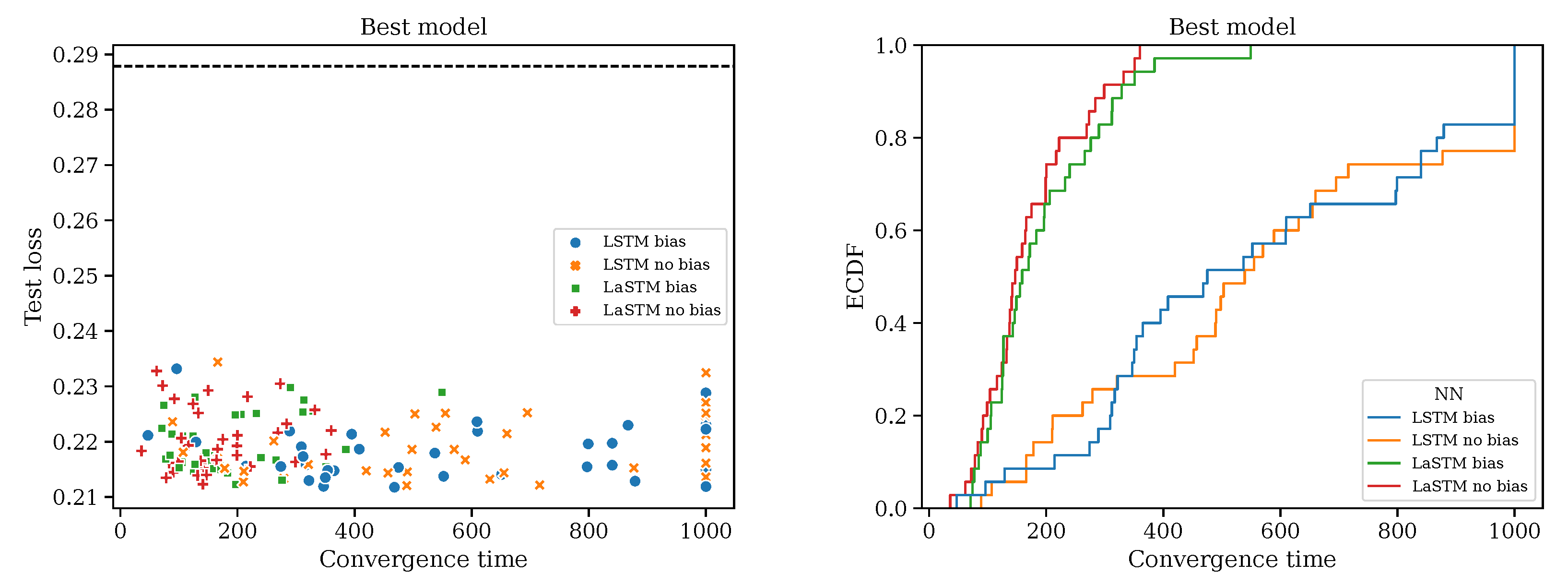
Figure 3 suggests to select the groups of good models, since the validation loss distribution is bimodal and the test losses are roughly proportional to validation losses. To select models whose validation loss belongs in the lower peak, we compute nine quantiles q ( p ) with a regular sequence of probabilities p = 0.1 , , 0.9 , and keep the models whose validation loss is smaller than the quantile corresponding to the maximum change between quantiles, a simple yet effective way to find well-separated peaks. We call these models the better ones in the following. This procedure allows for a fairer comparison between LSTMs and LaSTMs.
Table 1 reports the MSE of various model choices. LaSTMs are still better than LSTMs, even for larger N h . Figure 3 plots the average test loss of the models with a below-average validation loss versus N h and the sequence length. The test losses are now much closer, but LaSTMs still retain a sizeable advantage: their test losses are both lower on average and their fluctuations are much smaller.
Both the variability in results and the strange results for N h = 1 when biases are allowed in the computation of the internal states of LaSTMs can be traced back to training convergence problems. A simple way to ascertain the main difference between LaSTM and LSTM training is to measure the time it takes for them to converge, i.e., to reach the early stopping criterion. Figure 4 reports the fraction of models that have converged as a function of the number of epochs (limited to 1000). LSTMs need more epochs to be trained. We also found that the case N h = 1 and small T seq is hard to learn for this kind of architecture; the training of many models requires more than 1000 epochs to reach the early stopping criterion.

3.3. Best Model

Finally, let us investigate the test loss of the model with the best validation loss among the 20 models trained for each of the 140 hyperparameters/architecture choices. It turns out that under these conditions, LaSTMs and LSTMs exhibit essentially the same performance. What differentiates them however is the speed at which they learn. Let us plot the test loss versus the time of convergence for LSTMs and LaSTMs with and without biases (left plot in Figure 5). There is slight negative dependence between test losses and convergence times; the longer one learns, the better. Notably, the convergence times of LSTMs are spread all over the whole [ 1 , 1000 ] interval, while LaSTMs converge before 400 epochs. The right plot in Figure 5 displays the ECDF of the convergence times, which shows a sizeable difference between LSTMs and LaSTMs: whereas 20% of LSTMs models do not manage to converge before 1000 epochs, all LaSTMs do before 400, except one, when biases are allowed.
Thus, training a given number of models is significantly shorter with LaSTMs because they do not need to learn how to approximate the kernel K ( x ) . One also sees that models with internal biases converge slightly more slowly than those without them. We also wish to point out that because the fluctuation in validation losses among the trained models is much smaller for LaSTMs than for LSTMs, one needs to train fewer LaSTMs than LSTMs before finding a good one.

4. Discussion

Adding an explicit but flexible kernel structure to LSTMs brings significant improvements in almost every metric: the number of epochs needed to reach convergence, the overall prediction accuracy, and the accuracy variation between models at fixed parameters. There is a cost as LaSTMs have more trainable parameters than LSTMs for a given set pf hyperparameters, but doubling the number of timescales does not require one to double the number of trainable parameters thanks to the explicit kernel approximation structure. Although this paper focuses on LSTMs, the same idea can be applied to GRUs and α -RNNs in a straightforward way.
Our results mirror those of Rosenbaum and Zhang (2022): we also trained a single model on many volatility time series of various underlying asset types. This reflects the universality of volatility dynamics, a fact also hinted at by rough volatility (Gatheral et al. 2018) and multi-scale GARCH-like models (Zumbach 2015). By examining the performance of a larger population of trained models, we proposed a different way to select which models to use in the test phase.
While rough volatility and factor models are simple to calibrate, we found that even simple LSTMs can beat them, provided that one trains a population of models and selects the best one according to its validation loss. Using LSTMs for this purpose requires training more models over more epochs than using LaSTMs.
The fact that the best trained recurrent neural networks beat simpler models of volatility is probably linked to their abilities to learn to modulate the kernel over which the features are averaged, which would account for structural breaks better than a single kernel. Finally, volatility prediction can be further improved by adding some more features, such as prior knowledge of predictable special events, and possibly by using more complex neural architectures.

Author Contributions

Conceptualization, D.C.; methodology, D.C. and V.R.; software, D.C.; validation, D.C. and V.R.; formal analysis, D.C. and V.R.; investigation, D.C. and V.R.; resources, D.C. and V.R.; data curation, D.C. and V.R.; writing—original draft preparation, D.C. and V.R.; writing—review and editing, D.C. and V.R.; visualization, D.C. and V.R.; supervision, D.C. and V.R.; project administration, D.C. and V.R.; funding acquisition, D.C. and V.R. All authors have read and agreed to the published version of the manuscript.

Funding

V.R. acknowledges funding from the Association Nationale de la Recherche et de la Technologie (ANRT), grant number 2020/0622.

Data Availability Statement

Data and full source code to, including the Keras LaSTM class for Tensorflow 2.X, are available at https://github.com/damienchallet/LaSTM (accessed 14 May 2024).

Acknowledgments

We are grateful to Mathieu Rosenbaum and Julien Guyon for useful discussions. This work used HPC resources from the “Mésocentre” computing center of CentraleSupélec and École Normale Supérieure Paris-Saclay supported by CNRS and Région Île-de-France.

Conflicts of Interest

The authors declare no conflicts of interest. The funders had no role in the design of the study; in the collection, analyses, or interpretation of data; in the writing of the manuscript; or in the decision to publish the results.

Note

1
AEX, AORD, BFX, BSESN, BVLG, BVSP, DJI, FCHI, FTMIB, FTSE, GDAXI, GSPTSE, HSI, IBEX, IXIC, KS11, KSE, MXX, N225, NSEI, OMXC20, OMXHPI, OMXSPI, OSEAX, RUT, SMSI, SPX, SSEC, SSMI, STI, STOXX50E.

References

  1. Barndorff-Nielsen, Ole E., Peter Reinhard Hansen, Asger Lunde, and Neil Shephard. 2008. Designing realized kernels to measure the ex post variation of equity prices in the presence of noise. Econometrica 76: 1481–536. [Google Scholar]
  2. Bochud, Thierry, and Damien Challet. 2007. Optimal approximations of power laws with exponentials: Application to volatility models with long memory. Quantitative Finance 7: 585–89. [Google Scholar] [CrossRef]
  3. Challet, Damien, and Robin Stinchcombe. 2001. Analyzing and modeling 1 + 1d markets. Physica A: Statistical Mechanics and Its Applications 300: 285–99. [Google Scholar] [CrossRef]
  4. Cho, Kyunghyun, Bart van Merrienboer, Caglar Gulcehre, Dzmitry Bahdanau, Fethi Bougares, Holger Schwenk, and Yoshua Bengio. 2014. Learning phrase representations using rnn encoder–decoder for statistical machine translation. Paper Presented at the 2014 Conference on Empirical Methods in Natural Language Processing (EMNLP), Doha, Qatar, October 25–29; Cedarville: Association for Computational Linguistics, p. 1724. [Google Scholar]
  5. Cont, Rama. 2001. Empirical properties of asset returns: Stylized facts and statistical issues. Quantitative Finance 1: 223. [Google Scholar] [CrossRef]
  6. Corsi, Fulvio. 2009. A simple approximate long-memory model of realized volatility. Journal of Financial Econometrics 7: 174–96. [Google Scholar] [CrossRef]
  7. Dixon, Matthew, and Justin London. 2021. Financial forecasting with α-RNNs: A time series modeling approach. Frontiers in Applied Mathematics and Statistics 6: 551138. [Google Scholar] [CrossRef]
  8. Filipović, Damir, and Amir Khalilzadeh. 2021. Machine Learning for Predicting Stock Return Volatility. Swiss Finance Institute Research Paper. Zürich: Swiss Finance Institute, pp. 21–95. [Google Scholar]
  9. Ganesh, Prakhar, and Puneet Rakheja. 2018. Vlstm: Very long short-term memory networks for high-frequency trading. arXiv arXiv:1809.01506. [Google Scholar]
  10. Gatheral, Jim. 2016. Rough Volatility with Python. Available online: https://tpq.io/p/rough_volatility_with_python.html (accessed on 14 May 2024).
  11. Gatheral, Jim, Thibault Jaisson, and Mathieu Rosenbaum. 2018. Volatility is rough. Quantitative Finance 18: 933–49. [Google Scholar] [CrossRef]
  12. Gers, Felix A., Jürgen Schmidhuber, and Fred Cummins. 2000. Learning to forget: Continual prediction with LSTM. Neural Computation 12: 2451–71. [Google Scholar] [CrossRef] [PubMed]
  13. Guyon, Julien, and Jordan Lekeufack. 2023. Volatility is (mostly) path-dependent. Quantitative Finance 23: 1221–58. [Google Scholar] [CrossRef]
  14. Heber, Gerd, Asger Lunde, Neil Shephard, and Kevin Sheppard. 2022. Oxford-Man Institute’s Realized Library. Available online: https://realized.oxford-man.ox.ac.uk/ (accessed on 18 February 2021).
  15. Kim, Ha Young, and Chang Hyun Won. 2018. Forecasting the volatility of stock price index: A hybrid model integrating lstm with multiple GARCH-type models. Expert Systems with Applications 103: 25–37. [Google Scholar] [CrossRef]
  16. Lillo, Fabrizio, and J. Doyne Farmer. 2004. The long memory of the efficient market. Studies in Nonlinear Dynamics & Econometrics 8: 1–27. [Google Scholar] [CrossRef]
  17. Ohno, Kentaro, and Atsutoshi Kumagai. 2021. Recurrent neural networks for learning long-term temporal dependencies with reanalysis of time scale representation. Paper Presented at the 2021 IEEE International Conference on Big Knowledge (ICBK), Auckland, New Zealand, December 7–8; pp. 182–89. [Google Scholar]
  18. Palma, Wilfredo. 2007. Long-Memory Time Series: Theory and Methods. Hoboken: John Wiley & Sons. [Google Scholar]
  19. Palminteri, Stefano, Germain Lefebvre, Emma J Kilford, and Sarah-Jayne Blakemore. 2017. Confirmation bias in human reinforcement learning: Evidence from counterfactual feedback processing. PLoS Computational Biology 13: e1005684. [Google Scholar] [CrossRef] [PubMed]
  20. Resagk, Christian, Ronald du Puits, André Thess, Felix V Dolzhansky, Siegfried Grossmann, Francisco Fontenele Araujo, and Detlef Lohse. 2006. Oscillations of the large scale wind in turbulent thermal convection. Physics of Fluids 18: 095105. [Google Scholar] [CrossRef]
  21. Robinson, Peter M. 2003. Advanced Texts in Econometrics. In Time Series with Long Memory. Oxford: Oxford University Press. [Google Scholar]
  22. Rosenbaum, Mathieu, and Jianfei Zhang. 2021. Deep calibration of the quadratic rough heston model. arXiv arXiv:2107.01611. [Google Scholar]
  23. Rosenbaum, Mathieu, and Jianfei Zhang. 2022. On the universality of the volatility formation process: When machine learning and rough volatility agree. arXiv arXiv:2206.14114. [Google Scholar] [CrossRef]
  24. Thuerey, Nils, Philipp Holl, Maximilian Mueller, Patrick Schnell, Felix Trost, and Kiwon Um. 2021. Physics-based Deep Learning. arXiv arXiv:2109.05237. [Google Scholar]
  25. Zhao, Jingyu, Feiqing Huang, Jia Lv, Yanjie Duan, Zhen Qin, Guodong Li, and Guangjian Tian. 2020. Do RNN and LSTM have long memory? Paper Presented at the International Conference on Machine Learning, Online, July 13–18; pp. 11365–75. [Google Scholar]
  26. Zumbach, Gilles. 2010. Volatility conditional on price trends. Quantitative Finance 10: 431–42. [Google Scholar] [CrossRef]
  27. Zumbach, Gilles. 2015. Cross-sectional universalities in financial time series. Quantitative Finance 15: 1901–12. [Google Scholar] [CrossRef]
  28. Zumbach, Gilles, and Paul Lynch. 2001. Heterogeneous volatility cascade in financial markets. Physica A: Statistical Mechanics and Its Applications 298: 521–29. [Google Scholar] [CrossRef]
Figure 1. Volatility prediction. Upper plots: mean test loss vs. the memory cell dimension N h ( T seq = 40 ) ; lower plots: mean test loss vs. the sequence length T seq ( N h = 2 ). Left plots: LaSTMs with bias weights; right plots: LaSTMs with no bias weights. The dashed line is the average MSE of predictions made with rough volatility models.
Risks 12 00084 g001
Figure 2. Left plot: density of validation losses by architecture. Right plot: test loss vs. validation loss. Multiple volatility time series prediction. The dashed line is the average MSE of predictions made with vanilla rough volatility models.
Risks 12 00084 g002
Figure 3. Multiple volatility time series prediction test losses of the models with below-average validation losses. Upper plots: mean test loss vs. the memory cell dimension N h ( T seq = 100 ) ; lower plots: mean test loss vs. the sequence length T seq ( N h = 3 ). Left plots: LaSTMs with bias weights; right plots: LaSTMs with no bias weights. The dashed line is the average MSE of predictions made with rough volatility models.
Risks 12 00084 g003
Figure 4. Fraction of models with convergence before a given number of epochs. Left plot: N h = 1 , right plot: all N h ; multiple time series volatility prediction, T seq = 100 .
Risks 12 00084 g004
Figure 5. Left plot: test loss of the models with the best validation loss for all architectures and hyperparameter choices. Right plot: empirical cumulative distribution function of the convergence time for the four architecture choices. All values of N h and T seq ; multiple time series volatility prediction. The dashed line is the average MSE of predictions made with rough volatility models.
Risks 12 00084 g005
Table 1. Better models: average loss and standard deviation of the test losses, computed over all the values of N h and T seq .
ArchitectureBiasTest Loss
Average
Test Loss
Std Dev.
rough vol. 0.2880.015
LSTMyes0.2410.032
LSTMno0.2450.057
LaSTMyes0.2320.017
LaSTMno0.2300.015
Disclaimer/Publisher’s Note: The statements, opinions and data contained in all publications are solely those of the individual author(s) and contributor(s) and not of MDPI and/or the editor(s). MDPI and/or the editor(s) disclaim responsibility for any injury to people or property resulting from any ideas, methods, instructions or products referred to in the content.

