1. Introduction
Variable annuities (VAs), also known as segregated fund contracts in Canada, are a popular type of equity-linked insurance product often utilized as investment vehicles within North American retirement savings plans. VAs typically offer a range of guaranteed benefits aimed at providing protection, such as the Guaranteed Minimum Death Benefit (GMDB), Guaranteed Minimum Maturity Benefit (GMMB), Guaranteed Minimum Accumulation Benefit (GMAB), and Guaranteed Minimum Withdrawal Benefit (GMWB) (see, e.g.,
Hardy (
2003);
Ledlie et al. (
2008)). A substantial body of literature examines the stochastic modeling of embedded guarantees and their valuation in a fair market (risk-neutral) setting. However, the valuation of these embedded guarantees is complex due to the inherent complexity of diverse benefit designs. For example, GMDB guarantees a minimum amount to the policyholder upon death, exposing the insurer to various risks including investment, interest rate, mortality, and surrender risks. For a comprehensive overview of pricing, valuation, and risk management of individual VA contracts, we refer readers to existing literature, including
Feng et al. (
2022) and references therein. This paper primarily focuses on the valuation of large portfolios of VAs using statistical tools.
Due to the complex nature of the guarantees’ payoffs, closed-form solutions are often not feasible. Consequently, insurance companies extensively utilize Monte Carlo (MC) simulations for valuation and dynamic hedging purposes. However, valuing a large portfolio of Variable Annuity (VA) contracts using Monte Carlo simulation is notably time-intensive, as it requires projecting each contract across numerous scenarios over an extended time period (
Gan and Valdez 2018). To efficiently assess large VA portfolios within constrained timeframes or resources, numerous data mining techniques have been introduced. The predominant framework, metamodeling, integrates both supervised and unsupervised machine learning methods through several sequential modeling stages. It employs unsupervised learning to generate a small, representative dataset, followed by supervised learning to fit a predictive model to these data after valuation is completed. Literature reviews reveal various unsupervised learning algorithms such as the truncated fuzzy c-means algorithm (
Gan and Huang 2017), conditional Latin hypercube sampling (
Gan and Valdez 2018;
Minasny and McBratney 2006), and hierarchical
k-means clustering (
Gan and Valdez 2019). On the other hand, supervised learning approaches for VA portfolio valuation include kriging (
Gan 2013), GB2 (
Gan and Valdez 2018), group LASSO (
Gan 2018), and several tree-based methods (
Gweon and Li 2023;
Gweon et al. 2020;
Quan et al. 2021).
An alternative data mining approach is active learning (
Gweon and Li 2021;
Settles 2012), which involves iterative and adaptive data sampling and model training. Within this framework, the data sampling stage identifies a batch of informative policies, integrating these selected contracts into the existing representative data set. This augmented data set is then used for predictive model training. This cyclical process of sampling and updating continues until the allocated computational resources for portfolio assessment are exhausted. A prevalent strategy in active learning is uncertainty or ambiguity sampling (
Burbidge et al. 2007;
Settles and Craven 2008), which targets contracts where the current model shows significant predictive uncertainty.
Active learning methodologies have predominantly focused on classification problems, where the response variable is categorical. When the output variable is continuous, uncertainty can be quantified by prediction error, which can be decomposed into variance and squared bias. Current approaches to informativeness-based sampling for regression problems typically rely on prediction variance, under the assumption that the predictive model is approximately unbiased (
Burbidge et al. 2007;
Krogh and Vedelsby 1995;
Kumar and Gupta 2020). However, as noted by
Gweon et al. (
2020), there are practical instances where prediction bias is significant and cannot be overlooked. This recognition that prediction bias is a critical component of prediction error has spurred interest in using prediction bias as a measure of uncertainty in active learning. This paper explores the potential of bias-based sampling techniques in light of these findings.
To the best of our knowledge, this study represents pioneering research that explores the application of bias-based sampling in active learning for regression problems. We introduce a metric for bias-based sampling and investigate its utility under conditions where the predictive model exhibits significant or minimal bias. Empirical evaluations on a large synthetic VA portfolio with six response variables demonstrate the effectiveness of bias-based sampling using random forest (RF,
Breiman (
2001)), particularly compared to variance-based sampling. However, the effectiveness diminishes when bias reduction techniques for RF are implemented.
The remainder of the paper is structured as follows:
Section 2 reviews the active learning framework and discusses the estimation and application of prediction bias within this context.
Section 2.4 applies the proposed methods to the efficient valuation of a large synthetic VA dataset.
Section 3 concludes the paper.
2. Main Methodology
In this section, we propose several strategies to incorporate prediction bias into the active learning framework. We begin with a brief overview of the active learning framework and explore how prediction uncertainty is measured using random forest. Subsequently, we detail the integration of prediction bias into the modeling and sampling stages of active learning.
2.1. The Active Learning Framework for Large VA Valuation
Supervised statistical learning typically involves a one-time model training session using a complete set of labeled data. When large unlabeled data are available during the model training phase, active learning that uses both labeled and unlabeled data offers a viable alternative to traditional supervised learning. The primary objective of active learning is to iteratively enhance the predictive model by incorporating additional, informative samples selected from the pool of unlabeled data. This approach is particularly advantageous for rapidly valuing large VA portfolios because there are a large number of unlabeled contracts available during the model training process. As described by
Gweon and Li (
2021), the active learning process comprises the following steps:
- (1)
Formulate the initial representative data set by selecting a small subset from the entire portfolio, which can be chosen randomly.
- (2)
Determine the values of the response variable for the selected contracts using Monte Carlo simulation, thereby generating the labeled data necessary for training the predictive model.
- (3)
(Modeling stage) Train the predictive model using the labeled representative data.
- (4)
(Sampling stage) Apply the predictive model to the remaining set of unlabeled VA contracts to identify a subset of contracts whose information could significantly improve the model.
- (5)
Use a Monte Carlo simulation to label the newly selected contracts and integrate them into the existing set of labeled data, resulting in an expanded labeled dataset.
- (6)
Repeat steps (3) through (5) until specific stopping criteria are met, typically when the allocated time for valuation expires.
- (7)
Finalize the assessment by applying the updated predictive model to estimate the response values for the remaining unlabeled contracts.
The key part of an active learning algorithm is the selection of informative samples from the unlabeled data at each sampling iteration. Such informative samples lead to a great improvement in the current predictive model. Most existing approaches for informative sampling have been developed for classification problems and thus cannot be directly adapted to the VA valuation in which the target variables are continuous. Also, sampling a batch, instead of a single contract, is desirable for an efficient use of resources such as model runtime and parallel computing systems. Recently,
Gweon and Li (
2021) proposed batch-mode active learning approaches using random forest (
Breiman 2001) for an efficient valuation of large VA portfolios. To quantify the informativeness of each VA contract, they adopted the principle of Query-By-Committee (
Abe and Mamitsuka 1998;
Burbidge et al. 2007;
Freund et al. 1997) and used prediction ambiguity that is equivalent to the sample variance of bootstrap regression trees. They found that active learning can be highly effective when the informative samples are chosen by a weighted random sampling for which the sampling weights are proportional to prediction ambiguities.
A critical component of the active learning algorithm involves selecting informative samples from the unlabeled data during each iteration. These samples substantially enhance the accuracy and robustness of the existing predictive model. Traditional approaches for informative sampling, primarily developed for classification problems, are not directly applicable to VA valuation, where the target variables are continuous. Moreover, batch sampling—as opposed to selecting individual contracts—is desirable for an efficient use of resources, such as model runtime and parallel computing systems. Recently,
Gweon and Li (
2021) introduced batch-mode active learning strategies using random forest for the efficient valuation of large VA portfolios. To assess the informativeness of each contract, they implemented the Query-By-Committee principle (
Breiman 2001) and measured prediction ambiguity, akin to the sample variance of bootstrap regression trees. Their findings indicate that active learning can be exceptionally effective when informative samples are selected through weighted random sampling, where the weights are proportional to the prediction ambiguities.
2.2. Random Forests and Quantifying Prediction Bias
Suppose that a VA portfolio contains a total of
N contracts,
where each
represents a vector of feature variables associated with a contact. Random forest predicts the continuous response value
for each contract
using the regression form:
where
represents the underlying model, and
denotes random error. This modeling approach employs bootstrap regression trees (
Breiman 1984) to estimate the regression function, with foundational concepts detailed in
Gweon et al. (
2020) and
Quan et al. (
2021).
Let
L represent the labeled representative data containing
n VA contracts. Random forest consisting of
M regression trees constructs each regression tree
using the
m-th bootstrap sample
(
). The predicted response value for an unlabeled contract
is then derived by averaging across all
M bootstrap regression trees:
The effectiveness of random forest in VA portfolio valuation has been demonstrated in prior studies (
Gweon et al. 2020;
Quan et al. 2021).
Given the necessity of quantifying prediction uncertainty in active learning, we focus on the mean square error (MSE), defined as:
MSE is decomposed into the prediction (squared) bias and variance:
where the first term represents the squared bias and the second term, the variance.
Although the averaging technique in random forest greatly improves the predictive performance of regression trees by reducing the prediction variance, it does not influence the prediction bias. With the response values in a VA portfolio potentially exhibiting a highly skewed distribution,
Gweon et al. (
2020) identified that the prediction bias of random forest is not negligible.
Gweon et al. (
2020) showed a bias-correction technique (
Breiman 1999;
Zhang and Lu 2012) can effectively estimate and correct prediction bias. Specifically, prediction bias can be assessed by fitting an additional random forest model to the out-of-bag (OOB) errors of the trained model. The OOB prediction for a data vector
in the labeled set is defined as:
where
denotes the indicator function, and
is the number of bootstrap samples not containing
(i.e.,
). A subsequent model
is then trained where the response variable is the bias
, allowing the estimation of the prediction bias:
Combining the two random forest models, the bias-corrected random forest (BC-RF) predicts the response variable as the sum of
and
.
Gweon et al. (
2020) utilized the quantity
exclusively for mitigating prediction bias within the RF model as applied in the metamodeling framework. In the following section, we discuss how this bias is leveraged within the active learning process.
2.3. Using Prediction Bias in Active Learning Process
Our focus is to explore the integration of prediction bias,
, into the sampling stage of the active learning process. Instead of developing a new sampling methodology, we adopt the weighted random sampling (WRS) approach from
Gweon and Li (
2021), which is already established as effective. Utilizing prediction bias within this framework is straightforward. Under WRS with prediction bias, the active learning algorithm selects a batch of unlabeled contracts of size
d, where the sampling probability for a contract
within the unlabeled data set
U is defined as:
where
for
. We employ the squared bias terms to ensure non-negative sampling probabilities for all contracts and to facilitate a natural combination with the ambiguity component since the mean square error of the regression trees is the sum of variance and squared bias. We denote this approach as WRS-B to differentiate it from the ambiguity-based WRS (WRS-A), which calculates the weight as:
where the ambiguity score
represents the sample variance of the bootstrap regression trees, as detailed in
Gweon and Li (
2021).
When is WRS-B particularly effective in active learning? We posit that its effectiveness is contingent on the severity of prediction biases. If the predicted biases of the target response variable are significant, the weight in WRS-B acts as a measure of relative prediction uncertainty for the i-th contract. Conversely, if predictions are nearly unbiased, the bias estimates () may merely introduce noise and offer no substantial information, rendering the use of these scores a less effective uncertainty measure.
This analysis suggests that WRS-B could serve as a promising uncertainty measure for RF in the valuation of large VA portfolios in the presence of prediction biases, as demonstrated by
Gweon et al. (
2020). A deeper analysis is required for BC-RF, which predicts the response variable using two sequential RF models. In the
j-th iteration of active learning, the prediction by BC-RF is formulated as:
where
is the response prediction by an RF model, and
is the predicted bias by a subsequent RF model. If the primary contribution of WRS-B to the enhancement of
in the
-th iteration is bias reduction, the updated model
will yield less biased predictions, potentially reducing the impact of
.
Furthermore, we need to examine the relative effectiveness of WRS-B compared to WRS-A. If prediction ambiguity and bias are highly correlated, both sampling approaches may yield similar outcomes. However, if they are not, the samples selected by WRS-B and WRS-A are likely to differ. Moreover, these two uncertainty components—ambiguity and bias—can be combined in various ways. Since their sum corresponds to the mean square error of the individual trees, another variant, WRS based on mean square error (WRS-MSE), uses the weight:
In
Section 2.4, we further explore the application of prediction bias in active learning across various settings.
2.4. Application in Large Variable Annuity Portfolio Valuation
2.5. Description of Data
The data utilized in this study comprises a synthetic dataset from
Gan and Valdez (
2017), containing 190,000 variable annuity (VA) contracts. These contracts are characterized by 16 explanatory variables (14 continuous and 2 categorical), as summarized in
Table 1. Each of the ten investment funds within the dataset is linked to one or more market indices, with the specific mappings to the five market indices detailed in
Table 2.
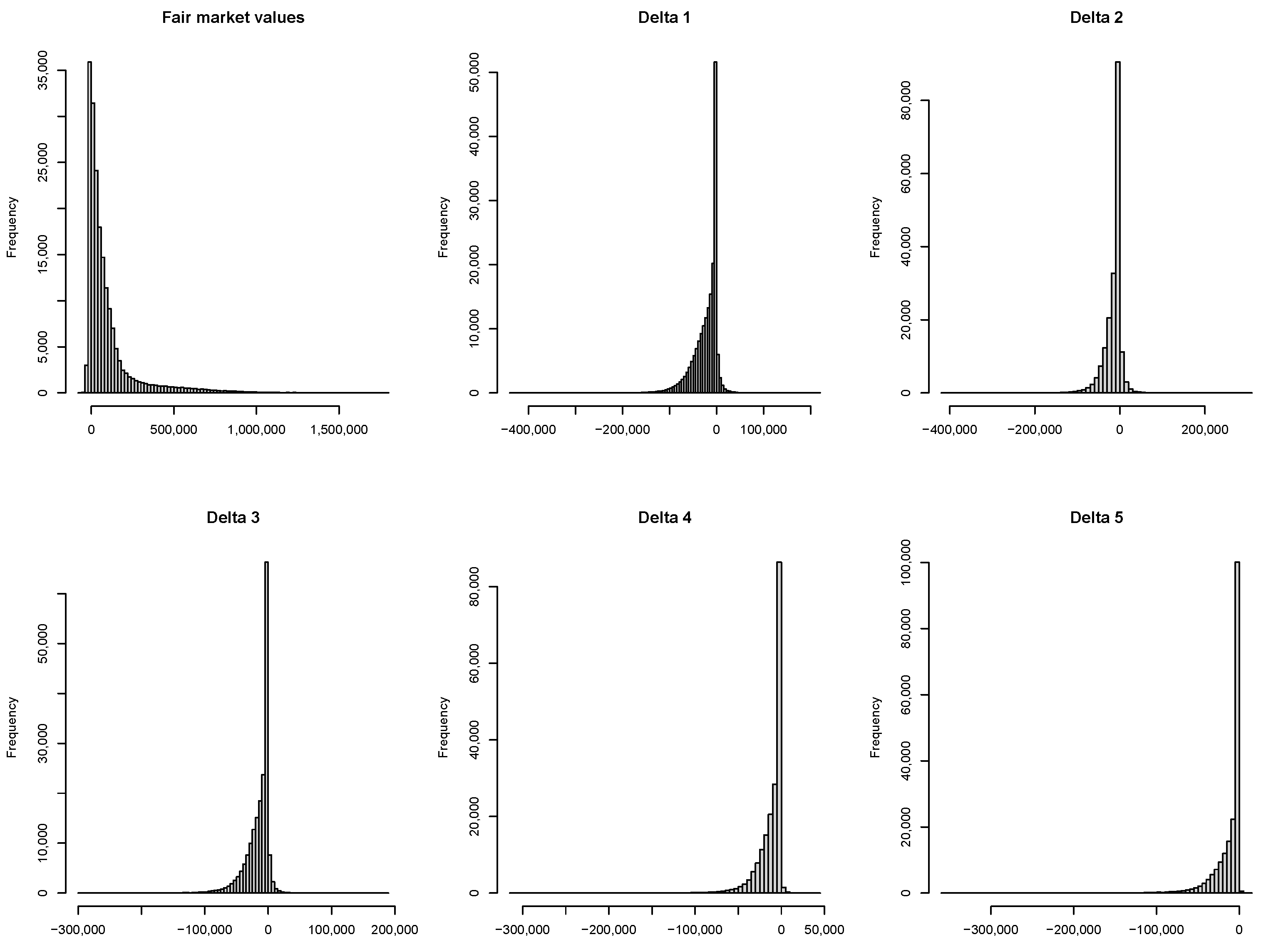
For the response variables, we analyze six variables: the fair market values (FMV) and five deltas. The FMV of a VA contract is defined as the difference between the guaranteed payoff and the guaranteed cost. The delta measures the rate of change of the theoretical option value relative to changes in the underlying asset’s price for a specific market index. The partial dollar deltas for a VA contract are calculated as follows:
where
denotes the partial account value linked to the
i-th market index and FMV is the fair market value as a function of partial account values. The partial dollar delta indicates the sensitivity of the guarantee value to fluctuations in the index, which is critical for determining appropriate hedge positions.
Figure 1 illustrates the distribution of the six response variables. Observations indicate that the distribution of FMV is significantly skewed to the right, while the distributions of the deltas are predominantly skewed to the left.
2.6. Experimental Setting
The active learning framework was initiated with a set of 100 representative contracts, selected through simple random sampling without replacement, to fit an initial regression model. For the response variable and the bias estimation, we employed two RF models, each using 300 regression trees to ensure stable performance, as supported by
Gweon et al. (
2020);
Quan et al. (
2021). Furthermore, consistent with findings from
Quan et al. (
2021), all 16 features were utilized in each binary split during tree construction, which has been shown to optimize performance for this dataset.
During each iteration of active learning, each sampling approach selected 50 contracts based on sampling probabilities. These contracts were then incorporated into the representative data set, and the RF models were subsequently updated with this augmented data. The iterative process was terminated once the representative data set expanded to include 800 contracts. To mitigate the impact of random variability, each active learning method was executed 20 times using different seeds. This experimental setup was consistently applied across all six response variables.
For each of the five partial deltas, it was noted that some contracts exhibited zero delta values, indicating no association with the relevant market index. Given that the link between a contract and its market index is predetermined, contracts with zero delta values were excluded from our prediction assessments to maintain the integrity and relevance of the analysis.
2.7. Evaluation Measures
To assess predictive performance, we employ several metrics:
, mean absolute error (
), and absolute percentage error (
):
and
where
. The
and
measure accuracy at the individual contract level, while
assesses portfolio-level accuracy, allowing for the offsetting of positive and negative prediction errors at the contract level. Higher values of
indicate better performance, whereas lower values of
and
are preferable.
2.8. Results
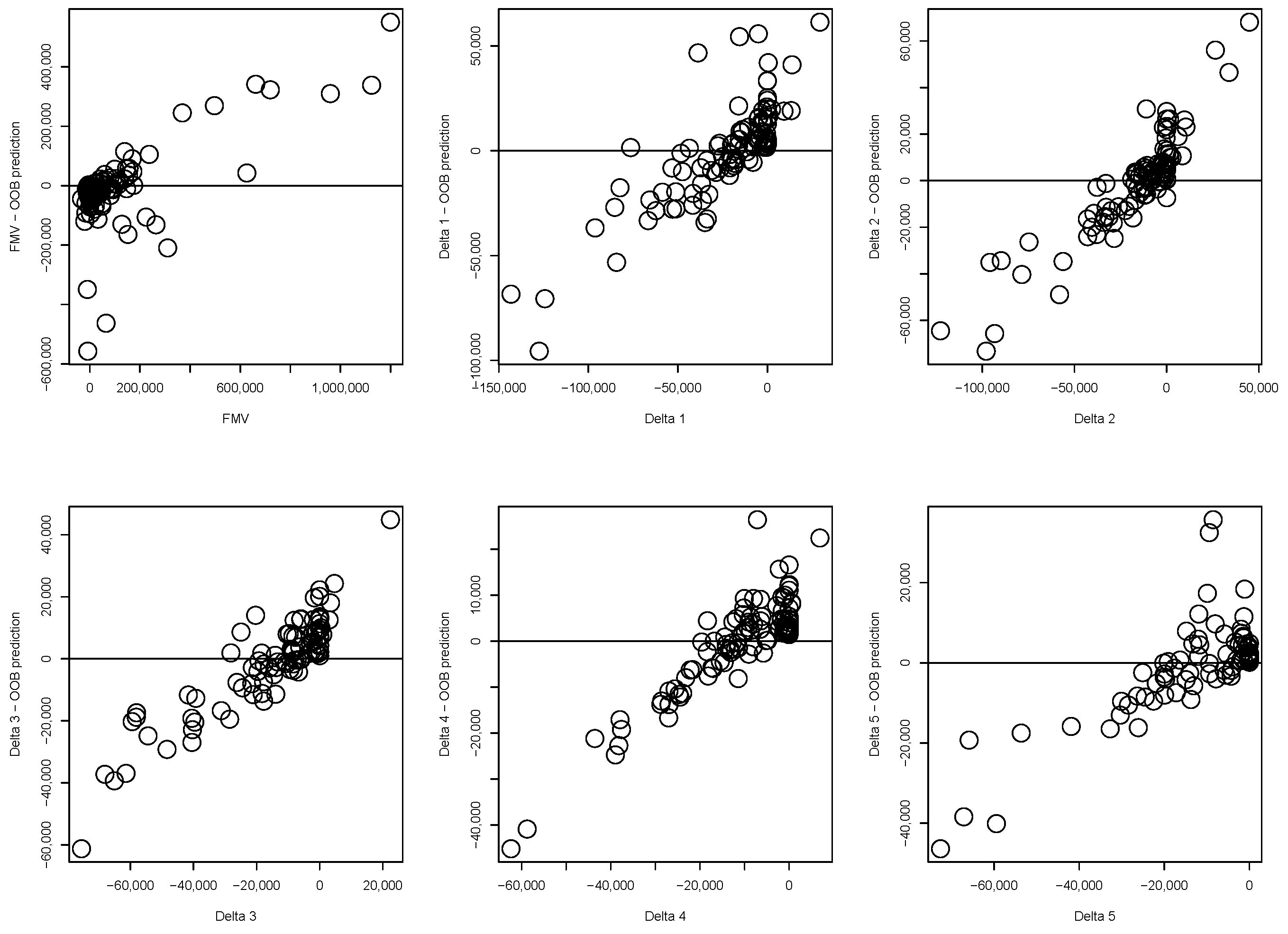
Initial investigations focused on identifying prediction bias across the six response variables.
Figure 2 presents the out-of-bag (OOB) error of RF as a function of the true response variable. An observed increasing or decreasing pattern suggests a likely severe bias in RF predictions of the remaining data, underscoring the potential of prediction bias as a valuable uncertainty measure in active learning.
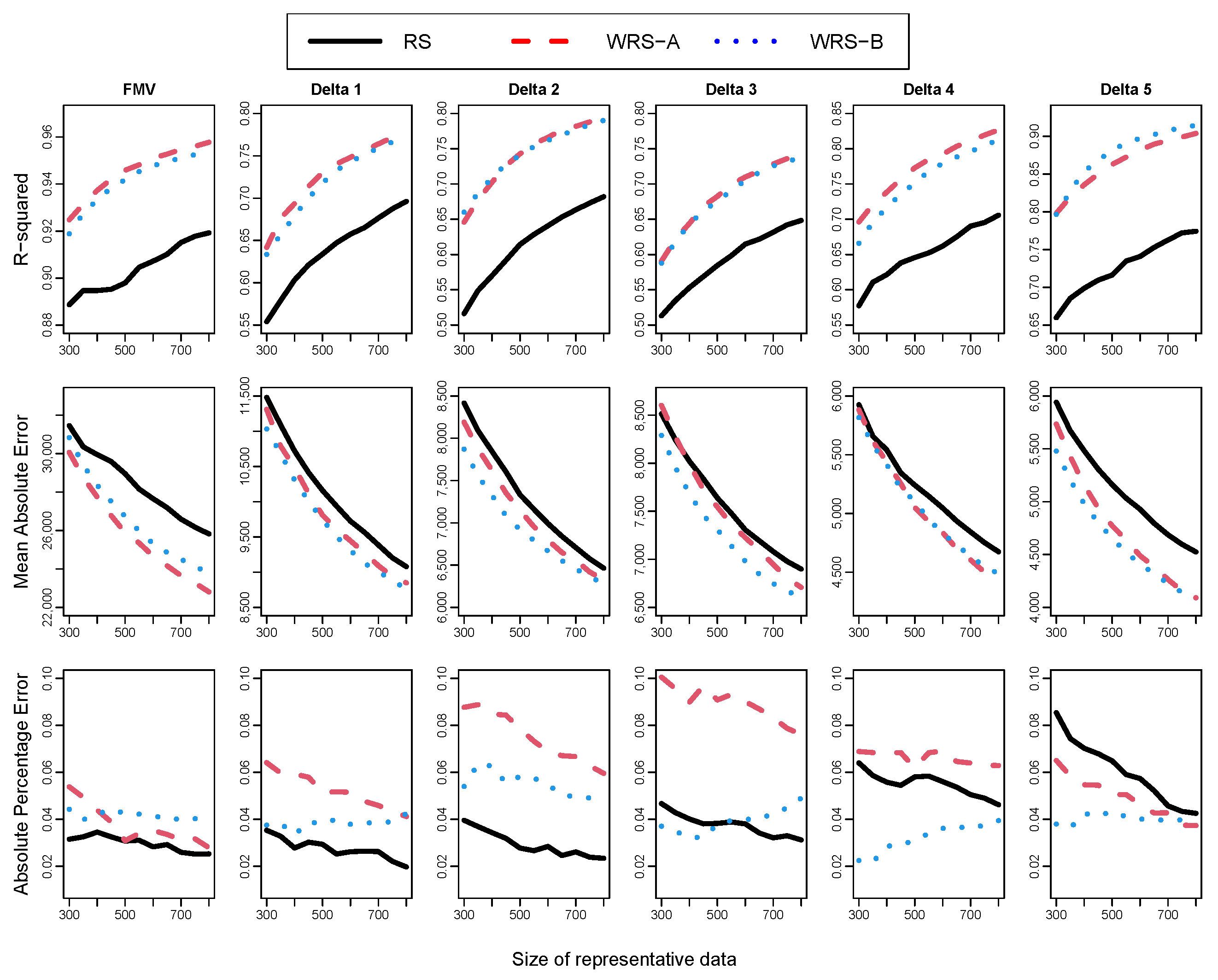
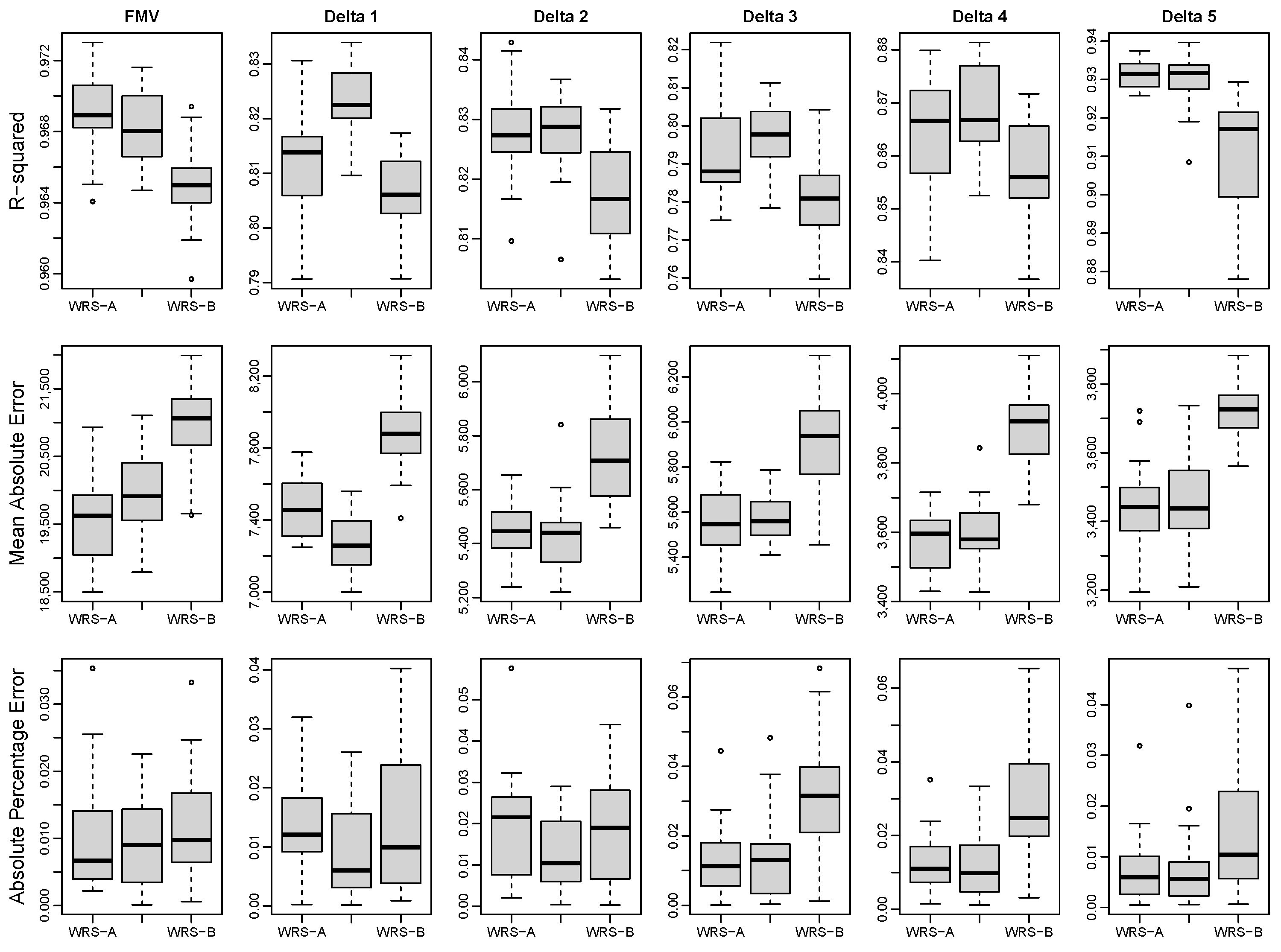
Figure 3 compares the performance of RF when using simple random sampling (RS), WRS-A and WRS-B. Both WRS-A and WRS-B consistently outperformed RS in terms of
and
across all response variables as the active learning process progressed. However, in terms of
, WRS-B tended to show more biased performance than RS. No clear advantage was observed between WRS-A and WRS-B; for instance, WRS-B yielded better
results than WRS-A for FMV, while WRS-A excelled over WRS-B for delta 5. The two sampling methods performed comparably for other response variables.
The observed correlations between ambiguity and squared bias ranged from 0.4 to 0.5, indicating that WRS-A and WRS-B selected somewhat different contracts during the sampling process.
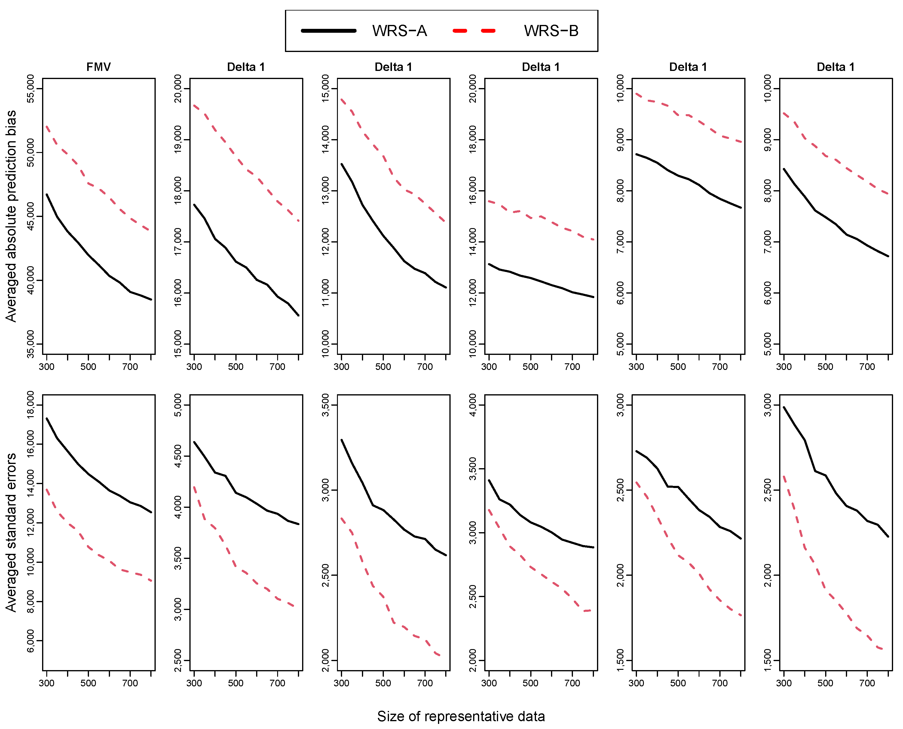
Figure 4 illustrates the average prediction standard errors and absolute biases under WRS-A and WRS-B, noting a gradual decrease across multiple iterations of active learning. Interestingly, WRS-A was more effective in reducing prediction standard errors than WRS-B, which excelled in diminishing prediction bias. These findings demonstrate distinct contributions of WRS-A and WRS-B to model improvement.
Subsequently, we explore the utilization of prediction bias in the modeling and sampling stages.
Table 3 compares the performance of RF with BC-RF under each sampling approach. The introduction of bias correction in the modeling stage significantly enhanced predictive performance across all metrics. Notably, the large APE previously observed in RF under both WRS-A and WRS-B were considerably reduced in BC-RF. Given these comparative results, BC-RF is recommended for use in active learning regardless of the sampling strategy.
We further examine the performance of BC-RF using WRS-A, WRS-B, and WRS-MSE in
Figure 5. Contrary to the inconclusive results observed with RF where no distinct advantage was noted between WRS-A and WRS-B, the implementation of BC-RF in the modeling stage generally showed WRS-A to be more effective than WRS-B in most situations. This observation aligns with earlier findings indicating that WRS-B substantially contributes to bias reduction in RF (refer to
Figure 4). Given that RF under WRS-B is relatively less biased compared to its counterpart under WRS-A, the subsequent application of BC-RF yields smaller gains from further bias reduction. This outcome is evidenced in
Table 4 and
Table 5, where the transition from RF to BC-RF exhibits more pronounced improvements under WRS-A.
Table 6 presents the runtime for each method until the representative VA contracts reached 800. When utilizing RF, WRS-A required approximately half the time compared to the other methods, as it did not involve an additional RF model for estimating prediction bias. In contrast, when BC-RF was employed, all sampling methods showed similar runtimes.
Interestingly, WRS-MSE often matched or exceeded the performance of WRS-A, as noted in the cases of Delta 1 and Delta 4. Considering that the computational times for WRS-MSE and WRS-A are nearly identical, these findings support a preference for WRS-MSE. Based on our analysis, we recommend employing BC-RF in the modeling stage alongside WRS-A or WRS-MSE in the sampling stage as an effective active learning strategy.
3. Concluding Remarks
In this study, we explored the integration of prediction bias within the active learning framework, specifically for the valuation of large variable annuity portfolios. Using a synthetic portfolio with six distinct response variables, we assessed the utility of prediction bias in both the modeling and sampling stages of active learning. Our experimental findings indicate that (a) employing prediction bias for uncertainty sampling (WRS-B) enhances performance of RF in terms of and , proving more effective than random sampling and as competitive as ambiguity-based uncertainty sampling (WRS-A); (b) uncertainty sampling based on prediction bias significantly contributes to the reduction of bias in RF; (c) prediction bias proves beneficial in the modeling stage across different sampling methods; and (d) WRS-B tends to be less effective than WRS-A when bias reduction is actively pursued during the modeling phase.
The batch-mode active learning framework necessitates an initial set of labeled representative data and a defined batch size. Although we employed simple random sampling to generate the initial datasets, alternative strategies involving unsupervised learning algorithms might be viable. Our tests with conditional Latin hypercube sampling indicated that the unsupervised learning method did not significantly influence the outcomes within the active learning framework. Furthermore, the batch size inversely affects the runtime of the active learning process; a larger batch size decreases the number of iterations needed to achieve the desired dataset size, as more data are labeled and incorporated at each step. Our analysis, initially based on a batch size of 50, showed that increasing this to 100 maintained similar performance across different sampling methods.
In conclusion, this paper highlights the potential of prediction bias as an effective uncertainty measure within active learning for actuarial applications. While our approach utilized RF, other statistical learning algorithms could be considered if prediction bias can be appropriately quantified. A comprehensive examination of bias-based active learning employing various statistical methods merits further investigation.


