Cyber Risk in Insurance: A Quantum Modeling

Abstract

In this research, we consider cyber risk in insurance using a quantum approach, with a focus on the differences between reported cyber claims and the number of cyber attacks that caused them. Unlike the traditional probabilistic approach, quantum modeling makes it possible to deal with non-commutative event paths. We investigate the classification of cyber claims according to different cyber risk behaviors to enable more precise analysis and management of cyber risks. Additionally, we examine how historical cyber claims can be utilized through the application of copula functions for dependent insurance claims. We also discuss classification, likelihood estimation, and risk-loss calculation within the context of dependent insurance claim data.

1. Introduction

The cyber insurance market is rapidly growing due to the effects of digital transformation in today’s world. Cyber risk, as both an emerging threat and an opportunity, is gaining prominence in the insurance landscape. Traditional insurance policies, such as those for motor vehicles or property, are increasingly incorporating cyber risks. This change is driven by the advent of connected and autonomous vehicles and the adoption of smart homes equipped with devices connected to servers and satellites. A major concern with traditional insurance policies is the undervaluation of cyber risk and ‘silent cyber’, which refers to previously unknown exposures that have neither been underwritten nor billed. Nevertheless, identifying and mitigating the exposure to silent cyber is possible (Aon 2018).

Cybercrime can manifest in many forms, including ransomware attacks, hacking, phishing, malware, spoofing, purchase fraud, theft of customer data, and tax fraud. This diversity, combined with the short history of available data and a rapidly evolving environment, makes handling cyber insurance claims and developing models significantly more complex than in traditional insurance (see, e.g., Dacorogna and Kratz 2022, 2023; Eling 2020; Tsohou et al. 2023). When evaluating common cyber risk scenarios, it is important to consider potential reputational damage, loss of confidential information, financial losses, regulatory fines, data privacy violations, data availability and integrity issues, contractual violations, and implications for third parties. After a cyber incident, the recovery time is crucial for mitigating business interruption. For example, the average recovery time for ransomware attacks is approximately 19 days (Tsohou et al. 2023).

Cyber insurance losses are generally categorized as ‘first party’ and ‘third party’. First-party losses are those that the insured party directly incurs. Third-party liability covers claims made by individuals or entities who allege they have suffered losses as a result of the insured’s actions (Romanosky et al. 2019; Tsohou et al. 2023). In the current research, we are focusing on first-party losses.

In today’s interconnected world, the perspective on risks is evolving. New emerging risks, technological advancements, and globalization increase the interdependence among risk parameters within the industry. For example, as demonstrated by COVID-19, a virus originating in one location can quickly escalate into a global pandemic, affecting insurance claims across distant regions. As a result, developing dependent risk models plays a crucial role in achieving better pricing in the insurance industry. However, employing dependent risk models is more complex than using independent models in predictive analytics. In actuarial science, copula functions are frequently used to model such dependencies (see, e.g., Constantinescu et al. 2011; Eling and Jung 2018; Embrechts et al. 2003; Lefèvre 2021).

Our goal here is to treat cyber claim amounts as quantum data rather than classical data due to the assumed uncertainty in the number of cyber attacks. In this context, the number of claims does not always correspond to the number of events (cyber attacks), so we analyze the cyber data by assuming that a single cyber claim can result from more than one cyber attack. Quantum methods originate from physics and have since been applied in various fields of application. Much of the theory and applications can be found in the books Baaquie (2014); Chang (2012); Griffiths (2002); Parthasarathy (2012). We also mention some recent work related to our subject. Thus, the analysis of quantum data in finance and insurance is studied in Hao et al. (2019); Lefèvre et al. (2018). Copulas and quantum mechanics are explored in Al-Adilee and Nanasiova (2009); Zhu et al. (2023). Cyber insurance pricing and modeling with copulas are discussed, e.g., in Awiszus et al. (2003); Eling and Jung (2018); Herath and Herath (2011).

In this paper, we start with a study on quantum theory for non-commutative paths. Next, we analyze synthetic data using a data classification method and risk-error functions. Finally, we use a classical copula function to predict future dependent claims.

2. Quantum Claim Data

Historical claim data from traditional insurance policies can be considered as classical data as there is generally no uncertainty about the number and amounts of claims, except in the cases of fraud and misreporting. Cyber claims, however, differ from traditional insurance claims in several ways, as listed in

Table 1. Differences between traditional insurance and cyber insurance.

Insurance Types	Identification of Damage	Claim Number
Traditional insurance	Claims, in most cases, are reported shortly after the occurrence of the insured event	Claim is the result of a single event in general
Cyber insurance	Claims may be reported long after the breach or attack due to delayed detection	Claim can result from more than one cyber attack

. Therefore, they should be handled from a different perspective.

Cyber damage is often detected much later and may result from multiple cyber attacks originating from diverse sources. According to the Cost of a Data Breach Report IBM (2023), the average time taken to identify and contain a data breach in 2022 was 277 days. Thus, we assume that the number of claims was 1 when the damage was noticed after 277 days. However, this damage could have originated from multiple sources at various times during those days.

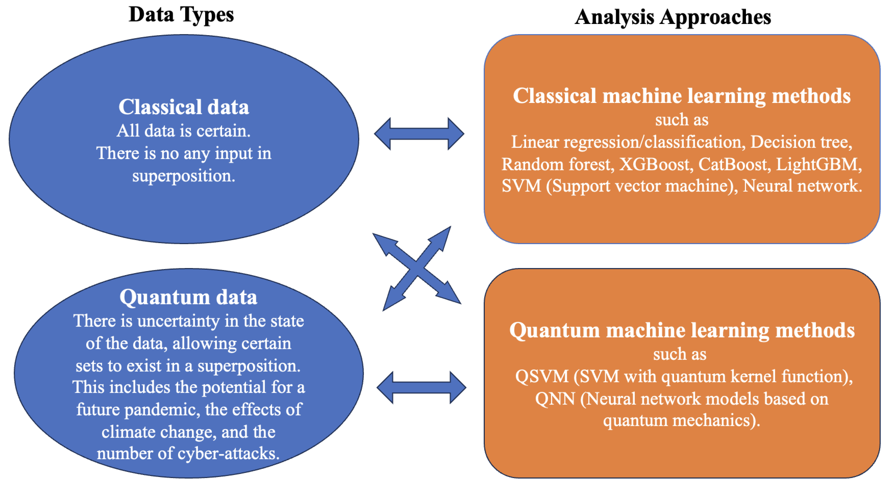
In Figure 1, the data types and analysis approaches are explained and illustrated (IBM 2024). While analyzing classical data using deterministic methods is widespread, the use of quantum algorithms—including quantum kernels and quantum neural networks—is becoming increasingly common. As previously noted, cyber insurance claims are considered under the assumption that they originate from several stochastic processes. Therefore, we will treat them as quantum data and examine them by computing likelihood and risk-loss functions within the context of dynamic classification.

3. Quantum for Non-Commutative Event Paths

Event paths and projectors. In a probabilistic setup, an event path $A_1,A_2,\dots ,A_k$ is modeled as a product of indicators as

$$I_{A_1}{I}_{A_2}\dots I_{A_k}=I_{A_1\cap A_2\cap \dots \cap A_k}.$$

Such indicators correspond to the projection operators in quantum theory. Recall that an operator P is called projector if P is self-adjoint and idempotent (i.e., $P^{*}=P$ and $P^2=P$). A basic projector is defined via a unit vector e by

$$P=|e\rangle \langle e|,$$

(1)

where $|x\rangle$ and $\langle x|$ are, respectively, column and row vectors that describe the quantum state of the system. They correspond to the bra-ket notation, also called Dirac notation. A general projector is then given by

$$P={\displaystyle \sum _i}|e_i\rangle \langle e_i|,$$

where $\left\{e_i\right\}$ denotes an orthonormal basis.

The probability of the system in the ground state e is measured by the expectation of (1). This expected value is obtained via a usual trace function $tr$ as

$$E\left(P\right)=E\left(|e\rangle \langle e|\right)=tr\left(\rho P\right),$$

(2)

where $\rho$ is a density operator which is a quantum state matrix of the system.

In quantum, a non-commutative version of the event path $A_1,A_2,\dots ,A_k$ is defined as a product of projectors as

$$P_1{P}_2\dots P_k.$$

Hereafter, the modeling is initiated by considering paths having the following product form

$$\begin{array}{ccccccc}\sigma ={\displaystyle \underbrace{P\cdots P}}& Q_1& {\displaystyle \underbrace{P\cdots P}}& Q_2& \dots & Q_{k-1}& {\displaystyle \underbrace{P\cdots P}}.\\ j_1& & j_2& & & & j_k\end{array}$$

(3)

In our context, $P=|e\rangle \langle e|$ is an event stating that the genuine customer has the right to exercise a financial claim if any, and the $Q_i$ are bounded self-adjoint operators indicating possible obstacles such as computer malfunctions, cyberattacks, criminal activities of a fraudster …

A self-adjoint operator Q is known to be bounded if it can be expanded as

$$Q={\displaystyle \sum _i}{\lambda }_i|e_i\rangle \langle e_i|,$$

(4)

where $e_i$ and ${\lambda }_i$ are the eigenvectors and eigenvalues of Q (i.e., $Q{e}_i={\lambda }_i{e}_i$). The probability of the measurement is extended by linearity of the expectation to

$$E\left(Q\right)=E\left({\displaystyle \sum _i}{\lambda }_i|e_i\rangle \langle e_i|\right)={\displaystyle \sum _i}{\lambda }_{i}E\left(|e_i\rangle \langle e_i|\right)=tr\left(\rho P_i\right),$$

(5)

after using (2).

Note, that the path $\sigma$ is not a projector in general. However, when $Q_i\equiv Q$ and Q is a projector, then $\sigma ={\left(PQP\right)}^{k-1}$ (provided that $j_1,\dots ,j_k\ge 1$) and it is a projector if and only if P and Q are commutative as follows from Halmos’ two projections theorem (see Bottcher and Spitkovsky 2010).

Quantum Risk Model. Let us first look at a genuine customer model similar to the one introduced in Lefèvre et al. (2018). A customer has the right to exercise financial claims. Any claim amount, if requested, is given by a fixed real number m which corresponds to a small claim for a short period of time. If not requested, the amount is 0.

Recall that an operator Z is observable if it is self-adjoint (i.e., $Z=Z^{*}$). For this model, the overall observable H is given by the following sum

$$H={\displaystyle \sum _j}{A}_j, \mathrm{where} A_j \mathrm{is} \mathrm{the} \mathrm{overall} \mathrm{capital} \mathrm{of} j \mathrm{potential} \mathrm{claims}.$$

This includes the actual amount modeled, with the help of the tensor product, as

$$ln{B}_m^{\otimes j}, \mathrm{where} B_m \mathrm{is} \mathrm{a} 2\times 2 \mathrm{self-adjoint} \mathrm{matrix} \mathrm{with} \mathrm{eigenvalues} e^m \mathrm{and} 1,$$

in agreement with Hao et al. (2019); Lefèvre et al. (2018). The exercise right is then described by the state projection $P_j$, thus

$$A_j=P_j\otimes ln{B}_m^{\otimes j},$$

(6)

so that H becomes

$$H={\displaystyle \sum _j}{P}_j\otimes ln{B}_m^{\otimes j}.$$

(7)

  Quantum Risk Model with Obstacles (called (O) model). This time, we hypothesize that the projector may be vulnerable to potential cyberattacks. We model the corresponding event as a path ${\sigma }_j$ of the form (1), using different parameters. Instead of (5), the j-th overall capital in this (O) model is then defined by

$$A_j^f={\sigma }_j\otimes ln{B}_m^{\otimes j}.$$

(8)

We now need to determine the overall observable $H^f$. This will be conducted using the following result.

Lemma 1.

A general path σ admits the representation

$$\sigma =aP,wherea=tr\left(\sigma \right).$$

(9)

Proof. 

By definition, $P=|e\rangle \langle e|$ in (1). Note, that $\sigma =aP$ in (9) necessarily implies $a=tr\left(\sigma \right)$ since

$$tr\left(\sigma \right)=tr\left(aP\right)=atr\left(|e\rangle \langle e|\right)=a.$$

From the decomposition (4) of Q, we obtain   

$$PQP=|e\rangle \langle e|\left({\displaystyle \sum _i}{\lambda }_i|e_i\rangle \langle e_i|\right)|e\rangle \langle e|=\left({\displaystyle \sum _i}{\lambda }_i\langle e|e_i\rangle \langle e_i|e\rangle \right)|e\rangle \langle e|\equiv cP,$$

where c is the term $(\dots )$. Thus, a direct computation gives, in obvious notation,

$$\sigma =\left(P{Q}_{1}P\right)\dots \left(P{Q}_{k-1}P\right)=(c_{1}P\dots c_{k-1}P)\equiv aP,$$

as announced in (9).    □

Returning to the (O) model, we have ${\sigma }_j=a_{j}P$ for all j by virtue of (9). Since $a_{j}ln{B}_m^{\otimes j}=ln{B}_{a_{j}m}^{\otimes j}$, the formula (8) of $A_j^f$ becomes

$$A_j^f=P_j\otimes ln{B}_{a_{j}m}^{\otimes j}.$$

(10)

From (10), the observable $H_f$ is thus given by

$$H_f={\displaystyle \sum _j}{A}_j^f={\displaystyle \sum _j}{P}_j\otimes ln{B}_{a_{j}m}^{\otimes j}.$$

(11)

For clarity, let us assume that all $a_j$ are equal to the same a. In other words, the obstacle activities are considered here to be homogeneous ((OH) case). From (7) and (11), we have proven the following result.

Proposition 1.

Define

$$H\left(t\right)={\Sigma }_j{P}_j\otimes ln{B}_t^{\otimes j},treal.$$

(12)

In the (OH) case,

$$H=H\left(m\right),and{H}_f=H\left(am\right)=aH\left(m\right).$$

(13)

More generally, we suppose there is one line of claims for the genuine customer model, yielding the observable $H=H\left(m\right)$, and n separate risk models with homogeneous obstacles, yielding the observables $H_f^i=H\left(b_{i}m\right)$, $i=1,\dots ,n$. This combined claim process is called (CC) model.

Corollary 1.

For the (CC) model, the overall observable is modeled by

$$\begin{array}{cc}\hfill & H\otimes H_f^1\otimes \dots \otimes H_f^n\hfill \\ \hfill & =H\left(m\right)\otimes H\left(b_{1}m\right)\otimes \dots \otimes H\left(b_{n}m\right).\hfill \end{array}$$

(14)

In Section 4, we will consider such a (CC) process with three possible obstacles, i.e., three (O) risk models, which leads to model the data using a sum of three stochastic processes. Before that, we present a few simple examples for illustration.

Example 1.

Consider two events A and B such that $A\cap B\ne \varnothing$. Let $I_A$ and $I_B$ be the indicators of these events. Suppose that a sequence of events gives the first eight outcomes $[0,0,1,1,0,1,0,0]$. In probability, the associated product of indicators is

$$I_A{I}_A{I}_B{I}_B{I}_A{I}_B{I}_A{I}_A=I_A^5{I}_B^3=I_B^3{I}_A^5,$$

because of the commutative property of indicators (see Lefèvre et al. 2017 for classical exchangeable sequences).

In quantum, $I_A$ and $I_B$ are replaced by projectors P and Q, respectively. Since projectors do not commute, in general, the associated product of projectors is as follows:

$$PPQQPQPP=PQPQP.$$

So, the order in which they are applied can provide different results.

Example 2.

For three events, we introduce the qubits $q_1,q_2,q_3$. The outcomes then are as follows:

$$|q_3\rangle \otimes \left(|q_2\rangle \otimes |q_1\rangle \right)=|q_3{q}_2{q}_1\rangle .$$

A basis for a qubit system is given by the eight states

$$|000\rangle ,|001\rangle ,|010\rangle ,|011\rangle ,|100\rangle ,|101\rangle ,|110\rangle ,|111\rangle ,$$

so that for a ψ system,

$$|\psi \rangle ={\alpha }_1|000\rangle +{\alpha }_2|001\rangle +{\alpha }_3|010\rangle +\dots +{\alpha }_8|111\rangle ,$$

where the ${\alpha }_j$ represent amplitudes of the states and satisfy ${\alpha }_1^2+\dots +{\alpha }_8^2=1$.

The probability of $[0,1,0]$ can be determined as in (5), via

$$\langle \psi |P_{010}|\psi \rangle =tr\left(\rho P_{010}\right),$$

where the density matrix ρ is given by $\left(|\psi \rangle \langle \psi |\right)$, i.e.,

$$\rho =\left({\rho }_{i,j}\right)=\left({\alpha }_i{\alpha }_j\right).$$

(15)

Sum of the matrices $P_{000},\dots ,P_{111}$ is an identity matrix $I_{8\times 8}$. Among them, $P_{010}$ is a matrix consisting entirely of zeros, except for the third element of the diagonal, which is 1. Using (15), we obtain

$$tr\left(\rho P_{010}\right)={\alpha }_3^2.$$

Example 3.

In the continuation of Example 1, consider for P and Q the following Jordan block matrices

$$P=\left(\begin{array}{cc}1& p\\ 0& 1\end{array}\right),Q=\left(\begin{array}{cc}1& q\\ 0& 1\end{array}\right),$$

where p and q take non-null values. We observe that $P^2\ne P$ and $Q^2\ne Q$, so they are not projectors.

Defining the density ρ by

$$\left(\begin{array}{cc}{p}_{11}& p_{12}\\ p_{21}& p_{22}\end{array}\right),$$

we then obtain

$$tr\left(\rho Q^n\right)=1+p_{21}nq,n\ge 1.$$

Basically, matrices with eigenvalues 1 cannot be treated as events, as this can lead to nonsensical results. How to deal with non-self-adjoint matrices is an important question; several methods are proposed in quantum modeling.

4. Quantum Approach to Cyber Insurance Claims

The overall compound claim is viewed here as the path resulting from a series of cyber attacks. Specifically, let $X_i\equiv S_i(\Delta t)$ denote the total cyber insurance claims occurred during successsive small time intervals $(t_i,t_i+\Delta t]$, over a horizon of length $n\Delta t$. Each claim $X_i$ is assumed to come from a combination of several stochastic processes, and the corresponding data are treated as quantum data. Let m be the mean of $X_i$ and $\lambda$ its frequency rate, so that $m\lambda$ measures the expected loss amount.

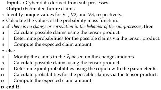
Our approach consists of two main steps: (i) learning patterns from existing data by dividing it into several stochastic processes, and (ii) using copula functions to generate data for estimating future claims. This section addresses point (i), while point (ii) will be discussed in the next section.

For illustration, we examine how to split historical claim data into (at most) three different stochastic processes. Naturally, if security vulnerabilities evolve over time, our current data may become less reliable. However, we can make it usable again by treating data as the result of combined processes and understanding their patterns.

Each claim $X_i$$(>0)$ is here the sum of the claims generated by three processes and can be expressed as

$$X_i={\displaystyle \sum _{i_1}}{Y}_{1,i_1}+{\displaystyle \sum _{i_2}}{Y}_{2,i_2}+{\displaystyle \sum _{i_3}}{Y}_{3,i_3},$$

(16)

where given any $j=1,2,3$, the claims $Y_{j,i_j}$, $i_j\ge 1$, are i.i.d. random variables with means $E\left(Y_j\right)=m_j$, and they occur independently at rates ${\lambda }_j$. This implies that

$$m\lambda \approx m_1{\lambda }_1+m_2{\lambda }_2+m_3{\lambda }_3.$$

The total expected claim amount per unit of time is shown in

Table 2. Generating processes with claim means and rates for (16).

Number of Processes	Claim Means and Rates	No Claim	One Claim	Two Claims	Three Claims
One stochastic process	Claim mean m and Claim frequency $\lambda$	0	m	$2m$	$3m$
Two stochastic processes	Claim means $m_1,m_2$ Claim frequencies ${\lambda }_1$ and ${\lambda }_2$, respectively	0	$m_1$, $m_2$	$m_1+m_2$, $2m_1$, $2m_2$	$3m_1$, $3m_2$, $2m_1+m_2$, $2m_2+m_1$,
Three stochastic processes	Claim means $m_1$, $m_2$ and $m_3$ Claim frequencies ${\lambda }_1$, ${\lambda }_2$ and ${\lambda }_3$, respectively	0	$m_1$, $m_2$, $m_3$	$2m_1$, $2m_2$, $2m_3$, $m_1+m_2$, $m_1+m_3$, $m_2+m_3$,	$3m_1$, $3m_2$, $3m_3$, $2m_1+m_2$, $2m_1+m_3$, $2m_2+m_1$, $2m_2+m_3$, $2m_3+m_1$, $2m_3+m_2$, $m_1+m_2+m_3$

when there are at most three generating processes.

Additionally, let us assume that $X_i$ is, for example, a combination of at most two claims per unit of time. In this case, (16) simplifies to

$$X_i={\displaystyle \sum _{i_1=1}^2}{Y}_{1,i_1}+{\displaystyle \sum _{i_2=1}^{2-i_1}}{Y}_{2,i_2}+{\displaystyle \sum _{i_3=1}^{2-i_1-i_2}}{Y}_{3,i_3},$$

(17)

where $X_i$ is positive but the $Y_{j,i_j}$’s can be zero. All possible scenarios for the mean claims are listed in

Table 3. Mean claims scenarios ranked in ascending order when $m_1<m_2<m_3$, for (17).

Schemes	Class 1	Class 2	Class 3	Class 4	Class 5	Class 6	Class 7	Class 8	Class 9
1	$m_1$	$m_2$	$m_3$	$2m_1$	$m_1+m_2$	$m_1+m_3$	$2m_2$	$m_2+m_3$	$2m_3$
2	$m_1$	$m_2$	$m_3$	$2m_1$	$m_1+m_2$	$2m_2$	$m_1+m_3$	$m_2+m_3$	$2m_3$
3	$m_1$	$2m_1$	$m_2$	$m_3$	$m_1+m_2$	$m_1+m_3$	$2m_2$	$m_2+m_3$	$2m_3$
4	$m_1$	$2m_1$	$m_2$	$m_1+m_2$	$m_3$	$m_1+m_3$	$2m_2$	$m_2+m_3$	$2m_3$
5	$m_1$	$2m_1$	$m_2$	$m_1+m_2$	$m_3$	$2m_2$	$m_1+m_3$	$m_2+m_3$	$2m_3$
6	$m_1$	$2m_1$	$m_2$	$m_1+m_2$	$2m_2$	$m_3$	$m_1+m_3$	$m_2+m_3$	$2m_3$
7	$m_1$	$m_2$	$2m_1$	$m_3$	$m_1+m_2$	$m_1+m_3$	$2m_2$	$m_2+m_3$	$2m_3$
8	$m_1$	$m_2$	$2m_1$	$m_3$	$m_1+m_2$	$2m_2$	$m_1+m_3$	$m_2+m_3$	$2m_3$
9	$m_1$	$m_2$	$2m_1$	$m_1+m_2$	$m_3$	$m_1+m_3$	$2m_2$	$m_2+m_3$	$2m_3$
10	$m_1$	$m_2$	$2m_1$	$m_1+m_2$	$m_3$	$2m_2$	$m_1+m_3$	$m_2+m_3$	$2m_3$
11	$m_1$	$m_2$	$2m_1$	$m_1+m_2$	$2m_2$	$m_3$	$m_1+m_3$	$m_2+m_3$	$2m_3$

in the case $m_1<m_2<m_3$. For example, if $m_1=2,m_2=5,m_3=50$, it is the 6-th scenario which is appropriate because the values in the classes are then in ascending order; if $m_1=8,m_2=10,m_3=40$, this is the 11-th scenario for the same reason.

Moreover,

Table 4. Total claims and their frequencies for (17).

${\mathit{X}}_{\mathit{i}}\equiv {\mathit{B}}_{\mathit{j}}$ Where	Frequencies ${\mathit{f}}_{\mathit{j}}$
$B_1=\left\{Y_{1,1}\right\}$	$f_1=e^{-{\lambda }_1}{\lambda }_1$
$B_2=\left\{Y_{2,1}\right\}$	$f_2=e^{-{\lambda }_2}{\lambda }_2$
$B_3=\left\{Y_{3,1}\right\}$	$f_3=e^{-{\lambda }_3}{\lambda }_3$
$B_4=\{Y_{1,1}+Y_{1,2}\}$	$f_4=e^{-{\lambda }_1}{\lambda }_1^2/2$
$B_5=\{Y_{1,1}+Y_{2,1}\}$	$f_5=e^{-{\lambda }_1}{e}^{-{\lambda }_2}{\lambda }_1{\lambda }_2$
$B_6=\{Y_{1,1}+Y_{3,1}\}$	$f_6=e^{-{\lambda }_1}{e}^{-{\lambda }_3}{\lambda }_1{\lambda }_3$
$B_7=\{Y_{2,1}+Y_{2,2}\}$	$f_7=e^{-{\lambda }_2}{\lambda }_2^2/2$
$B_8=\{Y_{2,1}+Y_{3,1}\}$	$f_8=e^{-{\lambda }_2}{e}^{-{\lambda }_3}{\lambda }_2{\lambda }_3$
$B_9=\{Y_{3,1}+Y_{3,2}\}$	$f_9=e^{-{\lambda }_3}{\lambda }_3^2/2$

gives the corresponding total claims $B_j$, $j=1,\dots ,9$, and their frequencies $f_j$, the probabilities of occurrence being ${\delta }_j=f_j/(f_1+\dots +f_9)$.

4.1. Hamiltonian Operator

Observable quantities are represented by self-adjoint operators. In the paper Lefèvre et al. (2018), we showed how to analyze such data using the quantum spectrum. In quantum mechanics, the spectrum of an operator is precisely the set of eigenvalues which correspond to observables for certain Hermitian operators/self-adjoint matrices.

Consider the model (17) with three processes and at most two claims per unit of time. We define the corresponding Hamiltonian observable operator by the following tensorial product

$$H=P_1\otimes ln(B\otimes I_3)+P_2\otimes ln\left(B^{\otimes 2}\right),$$

(18)

where $P_1$ and $P_2$ are the operators for one and two claims occurrences which are defined by the $2\times 2$ matrices

$$P_1=\left(\begin{array}{cc}1& 0\\ 0& 0\end{array}\right),\mathrm{and}{P}_2=\left(\begin{array}{cc}0& 0\\ 0& 1\end{array}\right),$$

B is the operator for the claim amount on a jump which is defined by the $3\times 3$ matrix

$$B=\left(\begin{array}{ccc}{e}^{m_1}& 0& 0\\ 0& e^{m_2}& 0\\ 0& 0& e^{m_3}\end{array}\right),$$

and $I_3$ is the identity operator of dimension 3 (ln is just applied to diagonal elements of the matrices).

The two terms of claim amounts in (18) are the diagonal $9\times 9$ matrices

$$\begin{array}{cc}\hfill & B\otimes I_3=diag\left(e^{m_1},e^{m_1},e^{m_1},e^{m_2},e^{m_2},e^{m_2},e^{m_3},e^{m_3},e^{m_3}\right),\hfill \\ \hfill & B^{\otimes 2}=diag\left(e^{2m_1},e^{m_1+m_2},e^{m_1+m_3},e^{m_2+m_1},e^{2m_2},e^{m_2+m_3},e^{m_3+m_1},e^{m_3+m_2},e^{2m_3}\right).\hfill \end{array}$$

Therefore, H is a self-adjoint $18\times 18$ matrix with eigenvalues

$$\begin{array}{cc}\hfill & m_1,m_1,m_1,m_2,m_2,m_2,m_3,m_3,m_3,2m_1,m_1+m_2,m_1+m_3,m_2+m_1,\hfill \\ \hfill & 2m_2,m_2+m_3,m_3+m_1,m_3+m_2,2m_3,\hfill \end{array}$$

so its spectrum has nine distinct eigenvalues

$$m_1,m_2,m_3,2m_1,m_1+m_2,2m_2,m_1+m_3,m_2+m_3,2m_3.$$

(19)

The Hamiltonian operator is given by (18) when the claim amount $X_i$ is strictly positive. If $X_i=0$, it is defined as

$$H=P_0\otimes ln(B\otimes O_3)+P_1\otimes ln(B\otimes I_3)+P_2\otimes ln\left(B^{\otimes 2}\right),$$

where

$$P_0=\left(\begin{array}{ccc}1& 0& 0\\ 0& 0& 0\\ 0& 0& 0\end{array}\right),P_1=\left(\begin{array}{ccc}0& 0& 0\\ 0& 1& 0\\ 0& 0& 0\end{array}\right),P_2=\left(\begin{array}{ccc}0& 0& 0\\ 0& 0& 0\\ 0& 0& 1\end{array}\right),and{O}_3=\left(\begin{array}{ccc}0& 0& 0\\ 0& 0& 0\\ 0& 0& 0\end{array}\right).$$

In the following, we assume $X_i>0$ and will thus use the Hamiltonian operator (18).

4.2. Likelihood and Risk Functions

First, we classify the data with respect to the eigenvalues (19) of the operator (18) and label them. The order of two successive claims in a unit of time is ignored. The different classes are listed below:

$$\begin{array}{cc}\hfill & C_{B_1}=\left\{m_1\right\},C_{B_2}=\left\{m_2\right\},C_{B_3}=\left\{m_3\right\},C_{B_4}=\left\{2m_1\right\},C_{B_5}=\{m_1+m_2\},\hfill \\ \hfill & C_{B_6}=\{m_1+m_3\},C_{B_7}=\left\{2m_2\right\},C_{B_8}=\{m_2+m_3\},C_{B_9}=\left\{2m_3\right\}.\hfill \end{array}$$

Using the Maxwell–Boltzmann statistics, the associated likelihood function $L(m_1,m_2,m_3)$ is given by

$$L(m_1,m_2,m_3)={\left({\delta }_1\right)}^{\#C_{B_1}}{\left({\delta }_2\right)}^{\#C_{B_2}}{\left({\delta }_3\right)}^{\#C_{B_3}}{\left({\delta }_4\right)}^{\#C_{B_4}}{\left({\delta }_5\right)}^{\#C_{B_5}}{\left({\delta }_6\right)}^{\#C_{B_6}}{\left({\delta }_7\right)}^{\#C_{B_7}}{\left({\delta }_8\right)}^{\#C_{B_8}}{\left({\delta }_9\right)}^{\#C_{B_9}},$$

where $\#C_{B_j}$ are the numbers of claims in class $C_{B_j}$, and ${\delta }_j$ are the normalized frequencies of Table 4 for the three Poisson processes.

Finally, the risk function $F(m_1,m_2,m_3)$ is calculated via the square distance (${\displaystyle \sum _{i\ge 1}}{|x_i-x_i^{\prime }|}^2$), or the Gaussian (squared exponential) distance (${\displaystyle \sum _{i\ge 1}}exp(-\gamma |x_i-x_i^{\prime }{|}^2)$, $\gamma \in {\mathbb{R}}^{+}$). For the square distance kernel, the risk function is here

$$\begin{array}{cc}\hfill & F(m_1,m_2,m_3)={\delta }_1{\displaystyle \sum _{x_i\in C_{B_1}}}|x_i-m_1{|}^2+{\delta }_2{\displaystyle \sum _{x_i\in C_{B_2}}}|x_i-m_2{|}^2+{\delta }_3{\displaystyle \sum _{x_i\in C_{B_3}}}{|x_i-m_3|}^2\hfill \\ \hfill & +{\delta }_4{\displaystyle \sum _{x_i\in C_{B_4}}}|x_i-2m_1{|}^2+{\delta }_5{\displaystyle \sum _{x_i\in C_{B_5}}}|x_i-(m_1+m_2){|}^2+{\delta }_6{\displaystyle \sum _{x_i\in C_{B_6}}}{|x_i-(m_1+m_3)|}^2\hfill \\ \hfill & +{\delta }_7{\displaystyle \sum _{x_i\in C_{B_7}}}|x_i-2m_2{|}^2+{\delta }_8{\displaystyle \sum _{x_i\in C_{B_8}}}|x_i-(m_2+m_3){|}^2+{\delta }_9{\displaystyle \sum _{x_i\in C_{B_9}}}{|x_i-2m_3|}^2,\hfill \end{array}$$

and for the Gaussian distance kernel,

$$\begin{array}{cc}\hfill & F(m_1,m_2,m_3)={\delta }_1{\displaystyle \sum _{x_i\in C_{B_1}}}{e}^{-|x_i-m_1{|}^2}+{\delta }_2{\displaystyle \sum _{x_i\in C_{B_2}}}{e}^{-|x_i-m_2{|}^2}+{\delta }_3{\displaystyle \sum _{x_i\in C_{B_3}}}{e}^{-|x_i-m_3{|}^2}\hfill \\ \hfill & +{\delta }_4{\displaystyle \sum _{x_i\in C_{B_4}}}{e}^{-|x_i-2m_1{|}^2}+{\delta }_5{\displaystyle \sum _{x_i\in C_{B_5}}}{e}^{-|x_i-(m_1+m_2){|}^2}+{\delta }_6{\displaystyle \sum _{x_i\in C_{B_6}}}{e}^{-|x_i-(m_1+m_3){|}^2}\hfill \\ \hfill & +{\delta }_7{\displaystyle \sum _{x_i\in C_{B_7}}}{e}^{-|x_i-2m_2{|}^2}+{\delta }_8{\displaystyle \sum _{x_i\in C_{B_8}}}{e}^{-|x_i-(m_2+m_3){|}^2}+{\delta }_9{\displaystyle \sum _{x_i\in C_{B_9}}}{e}^{-|x_i-2m_3{|}^2}.\hfill \end{array}$$

To minimize such a risk value, we perform optimization on all possible values of $(m_1,m_2,m_3)$. Additionally, we determine boundaries using the neighborhood approach.

4.3. Illustration

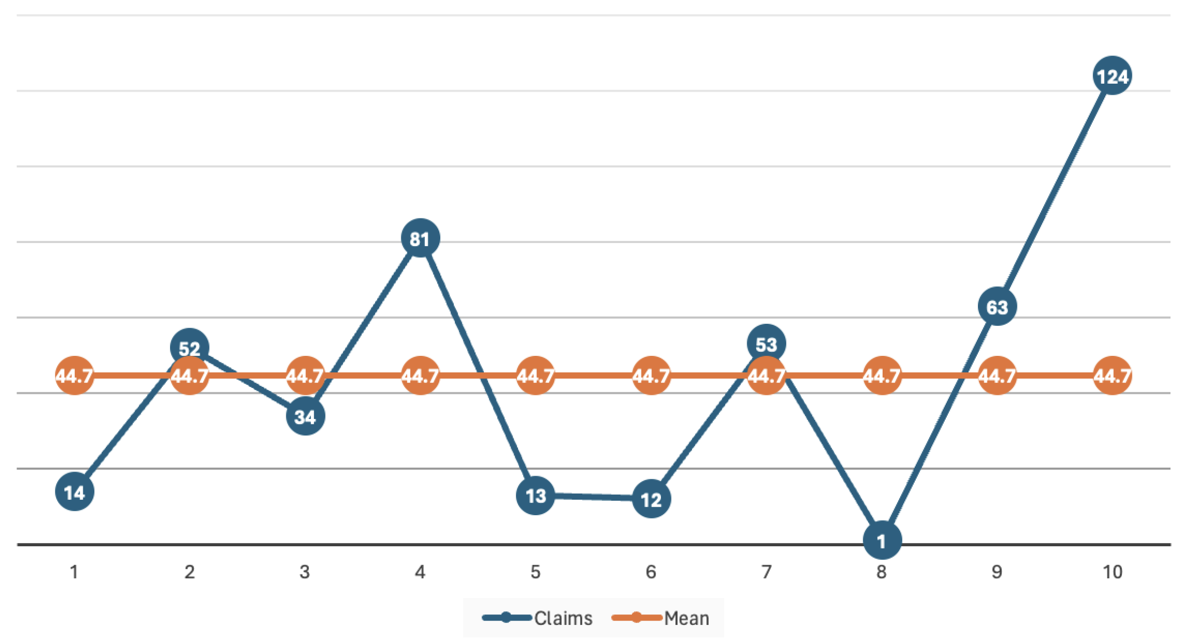
Let us consider the following dataset

$$\{14,52,34,81,13,12,53,1,63,124\}.$$

The main reason for choosing a small dataset size is only to simplify the demonstration of the example. Our algorithm can of course be applied to large datasets.

Table 5. Means and rates obtained with different distance kernels.

Kernels	${\mathit{m}}_1$	${\mathit{m}}_2$	${\mathit{m}}_3$	${\mathit{\lambda }}_1$	${\mathit{\lambda }}_2$	${\mathit{\lambda }}_3$	$\mathit{m}\mathit{\lambda }\approx$ ${\mathit{m}}_1{\mathit{\lambda }}_1+{\mathit{m}}_2{\mathit{\lambda }}_2+{\mathit{m}}_3{\mathit{\lambda }}_3$
Square distance kernel	6	26	59	0.9	0.6	0.4	44.6
With the neigborhood method	6	28	56	0.9	0.2	0.6	44.6
Gaussian distance kernel	5	11	55	0.3	0.6	0.6	41.1
With the neigborhood method	5	16	52	0.3	0.7	0.6	43.9

shows the means $m_1,m_2,m_3$ and the rates ${\lambda }_1,{\lambda }_2,{\lambda }_3$ for the three processes, obtained using the two previous distance kernels. Neighborhood optimization is conducted here by perturbing the boundaries between classes with $ϵ\in (-2,2)$. Of course, it is possible to achieve better results with an advanced optimization technique.

As expected, using different kernels with nearest neighbor approaches influence the results. For the current analysis, we applied the squared distance kernel and thus obtain $m_1=6$, $m_2=26$, $m_3=59$ (which corresponds to scenario 6 of Table 3). In addition, the dataset is distributed in the nine classes according to the distribution indicated in

Table 6. Classification of the data set for $m_1=6$, $m_2=26$, $m_3=59$.

${\mathit{C}}_{{\mathit{B}}_1}$	${\mathit{C}}_{{\mathit{B}}_2}$	${\mathit{C}}_{{\mathit{B}}_3}$	${\mathit{C}}_{{\mathit{B}}_4}$	${\mathit{C}}_{{\mathit{B}}_5}$	${\mathit{C}}_{{\mathit{B}}_6}$	${\mathit{C}}_{{\mathit{B}}_7}$	${\mathit{C}}_{{\mathit{B}}_8}$	${\mathit{C}}_{{\mathit{B}}_9}$
$m_1$	$m_2$	$m_3$	$2m_1$	$m_1+m_2$	$m_1+m_3$	$2m_2$	$m_2+m_3$	$2m_3$
$\left[1\right]$	$\left[\right]$	$\left[\right]$	$[14,13,12]$	$\left[34\right]$	$\left[63\right]$	$[52,53]$	$\left[81\right]$	$\left[124\right]$

. For this classification, midpoint values are used to define class boundaries. Note, that these boundaries are dynamic and change in response to the values of $m_1$, $m_2$, $m_3$.

The classes containing two claims, i.e., $C_{B_4}=\left\{2m_1\right\}$, $C_{B_5}=\{m_1+m_2\}$, $C_{B_6}=\{m_1+m_3\}$, $C_{B_7}=\left\{2m_2\right\}$, $C_{B_8}=\{m_2+m_3\}$, $C_{B_9}=\left\{2m_3\right\}$, are separated with respect to the weights of $m_1$, $m_2$, $m_3$ as follows:

$$\begin{array}{cc}\hfill & \mathrm{for}{C}_{B_4},C_{B_7},C_{B_9}:\mathrm{weights}1/2,1/2,\mathrm{for}{C}_{B_5}:m_1/(m_1+m_2),m_2/(m_1+m_2),\hfill \\ \hfill & \mathrm{for}{C}_{B_6}:m_1/(m_1+m_3),m_3/(m_1+m_3),\mathrm{for}{C}_{B_8}:m_2/(m_2+m_3),m_3/(m_2+m_3).\hfill \end{array}$$

So, the two claims in $C_{B_4}$ of sum 14, for example, yield the amounts 7 and 7. For $C_{B_5}$, the sum 34 is subdivided into $6.38$ and $27.63$; for $C_{B_6}$, 63 becomes $5.82$ and $57.18$; for $C_{B_8}$, 81 yields $24.78$ and $56.23$.

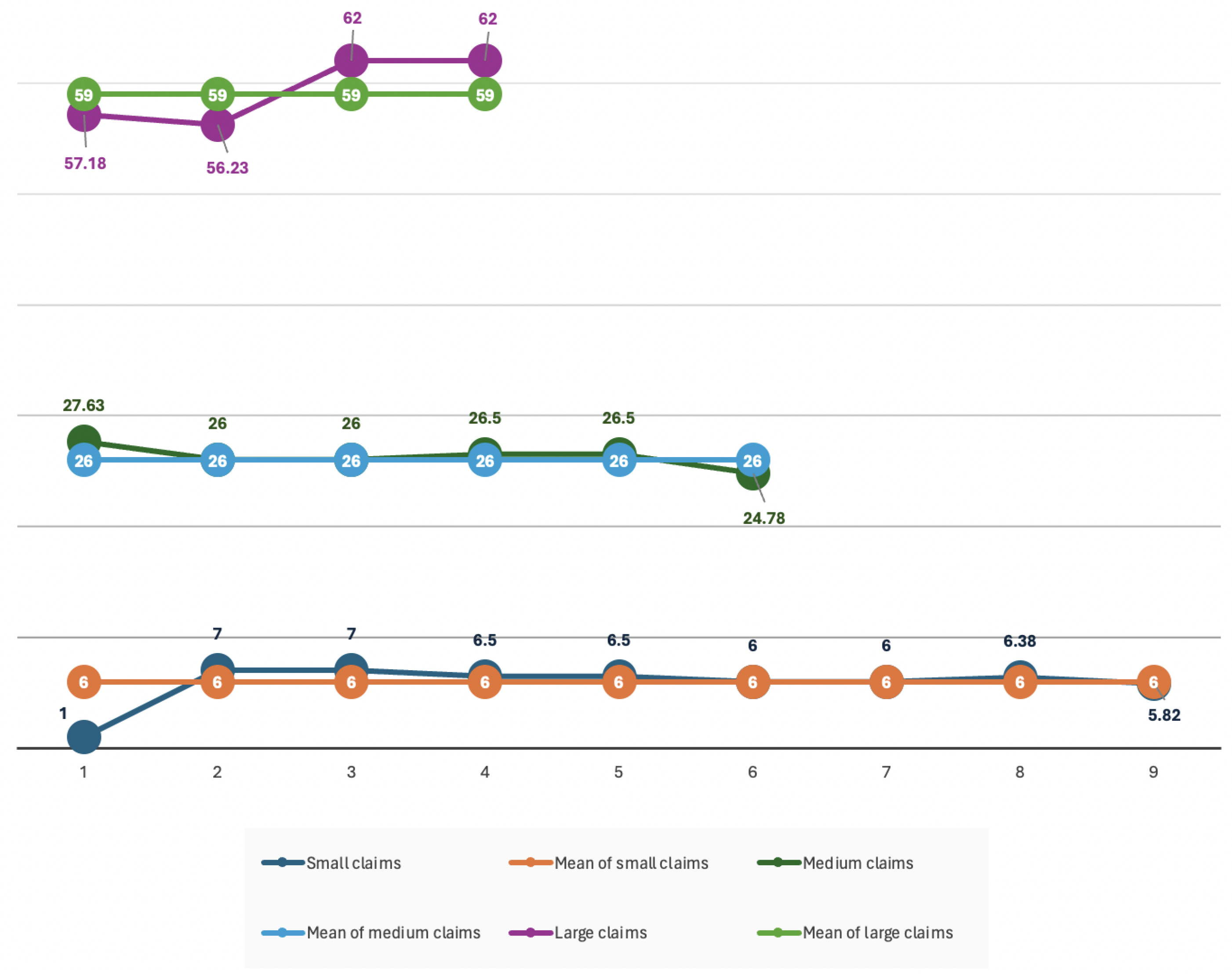
Following this method, the claims in the three processes are listed in

Table 7. Claims for the sub-processes.

Processes	Claims
1st process (Small claims)	$V_1=\{1,7,7,6.5,6.5,6,6,6.38,5.82\}$,
2nd process (Medium claims)	$V_2=\{27.63,26,26,26.5,26.5,24.78\}$,
3rd process (Large claims)	$V_3=\{57.18,56.23,62,62\}$.

and displayed with their means and frequencies in Figure 2. According to Table 5, the claim arrival rates for these processes are ${\lambda }_1=0.9$, ${\lambda }_2=0.6$, ${\lambda }_3=0.4$.

As shown in Figure 3 and Figure 4, the deviation from the mean in the sub-processes is minimized after the claims splitting and categorization process.

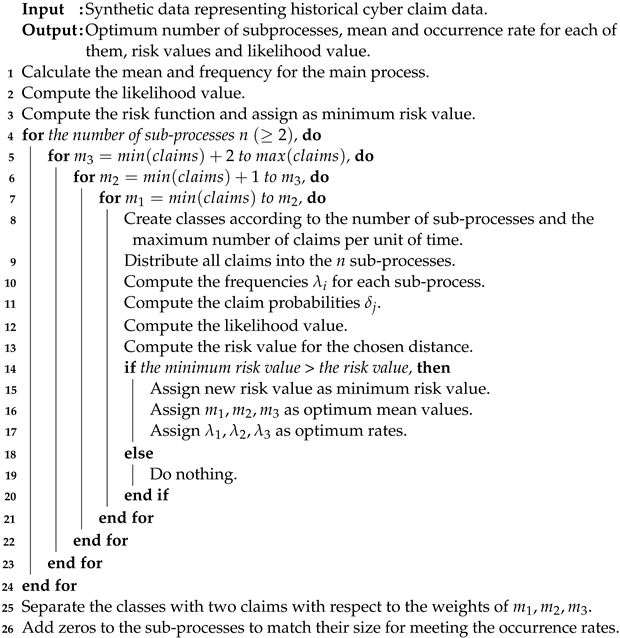
The detailed pseudo-code is provided by the Algorithm 1.

Algorithm 1: for splitting the main claim process and classifying the cyber data.

5. Generating Dependent Cyber Claims with Copulas

In the previous section, we analyzed a synthetic dataset by dividing the main claim process into three subprocesses. We are now able to estimate new claims by working precisely within this framework.

5.1. When the Sub-Processes Are Independent

Let us start by assuming that the behaviors of the subprocesses are always independent. Then, we can directly estimate the spectrum $\overline{V}$ of future cyber claims by

$$\begin{array}{cc}\hfill \overline{V}& \equiv ln\left(e^{{\overline{V}}_1}\otimes e^{{\overline{V}}_2}\otimes e^{{\overline{V}}_3}\right)\hfill \\ \hfill & =ln\left[\left(\begin{array}{c}{e}^{v_{1,1}}\\ \cdots \\ e^{v_{1,n_1}}\end{array}\right)\otimes \left(\begin{array}{c}{e}^{v_{2,1}}\\ \cdots \\ e^{v_{2,n_2}}\end{array}\right)\otimes \left(\begin{array}{c}{e}^{v_{3,1}}\\ \cdots \\ e^{v_{3,n_3}}\end{array}\right)\right],\hfill \end{array}$$

(20)

where ${\overline{V}}_i$, $i=1,2,3$, is the set of distinct elements $v_{i,j}$ from $V_i$, which are in number $n_i$. For example, in Section 4.3, $\overline{V_1}=\{1,7,6.5,6,6.38,5.82\}$ and $n_1=6$. So, the expected value of the spectrum is as follows

$$E\left(\overline{V}\right)={\displaystyle \sum _{k=1}^{n_1{n}_2{n}_3}}{\left(c\right)}_k{\left(\overline{V}\right)}_k,$$

where ${\left(\overline{V}\right)}_k$ is the k-th element of the column vector $\overline{V}$ (of size $n_1{n}_2{n}_3$), and ${\left(c\right)}_k$ denotes its probability mass function which is calculated through the vector c given by

$$\begin{array}{cc}\hfill c& \equiv p_{{\overline{V}}_1}\left(v_1\right)\otimes p_{{\overline{V}}_2}\left(v_2\right)\otimes p_{{\overline{V}}_3}\left(v_3\right)\hfill \\ \hfill & =\left(\begin{array}{c}P({\overline{V}}_1=v_{1,1})\\ \cdots \\ P({\overline{V}}_1=v_{1,n_1})\end{array}\right)\otimes \left(\begin{array}{c}P({\overline{V}}_2=v_{2,1})\\ \cdots \\ P({\overline{V}}_2=v_{2,n_2})\end{array}\right)\otimes \left(\begin{array}{c}P({\overline{V}}_3=v_{3,1})\\ \cdots \\ P({\overline{V}}_3=v_{3,n_3})\end{array}\right).\hfill \end{array}$$

Without change, $E\left(\overline{V}\right)\approx m$ since merging the separate claims should give us the same result. In conclusion, $\overline{V}$ in (20) applies in the independent case.

Of course, if the behaviors of the three processes change due to emerging technologies or risks, we may modify the claims associated with these processes accordingly as follows:

$$\overline{V}=ln\left[\left(\begin{array}{c}{e}^{v_{1,1}+{ϵ}_1}\\ \cdots \\ e^{v_{1,n_1}+{ϵ}_1}\end{array}\right)\otimes \left(\begin{array}{c}{e}^{v_{2,1}+{ϵ}_2}\\ \cdots \\ e^{v_{2,n_2}+{ϵ}_2}\end{array}\right)\otimes \left(\begin{array}{c}{e}^{v_{3,1}+{ϵ}_3}\\ \cdots \\ e^{v_{3,n_3}+{ϵ}_3}\end{array}\right)\right],$$

where ${ϵ}_i\in \mathbb{R}$, $i=1,2,3$, represents the amount of change in each subprocess.

5.2. When the Sub-Processes Can Be Correlated

Consider a scenario involving the presence of dependence effects over time. A practical way to predict future claims is then to use some copula functions. We briefly recall basic points in the theory of copulas. Let $(U_1,\dots ,U_n)$ be a vector of n random variables that are distributed uniformly on $(0,1)$. A copula C is the joint distribution function of such a vector, i.e.,

$$C(u_1,\dots ,u_n)=P(U_1\le u_1,\dots ,U_n\le u_n),u_1,\dots ,u_n\in (0,1).$$

In the particular degenerate case where the $U_i$ are independent, then $C(u_1,\dots ,u_n)=u_1\dots u_n$. Sklar’s key theorem states that the joint distribution function F of any continuous vector $(X_1,\dots ,X_n)$ having marginal distribution functions $F_i$ admits a unique copula representation as

$$F(x_1,\dots ,x_n)=C(F_1\left(x_1\right),\dots ,F_n\left(x_n\right)).$$

Now, a copula is called Archimedean if it has the simplified form

$$C(u_1,\dots ,u_n)={\varphi }^{-1}\left[\varphi \left(u_1\right)+\dots +\varphi \left(u_n\right)\right],u_1,\dots ,u_n\in [0,1],$$

for some univariate function $\varphi \left(x\right):[0,1]\to [0,\infty )$ which is completely monotonic with $\varphi \left(0\right)=\infty$ and $\varphi \left(1\right)=0$. Observe that in this case, the vector $(U_1,\dots ,U_n)$ is automatically exchangeable (in de Finetti sense). We note, however, that the symmetry of the distribution can be broken by making this vector only partially exchangeable (see Lefèvre 2021). One of the most common Archimedean copulas is the Clayton copula defined by

$$C_{\theta }(u_1,\dots ,u_n)={\left(max\{u_1^{-\theta }+\dots +u_n^{-\theta }-n+1,0\}\right)}^{-1/\theta },$$

(21)

where $\theta$ represents a positive parameter. Here, we will work precisely with this copula for $n=2$.

More precisely, we assume that there is dependence between claims coming from the first and second sub-processes, while claims originating from the third one remain independent. Then, we use the bivariate Clayton copula $C_{\theta }(u_1,u_2)$ given by (21) to model claims of these first two sub-processes. For a discrete version of the copula, we refer to Trivedi and Zimmer (2017) which provides its probability mass function, denoted $c_{\theta }(u_{1,j_1},u_{2,j_2})$, as

$$c_{\theta }(u_{1,j_1},u_{2,j_2})=C_{\theta }(u_{1,j_i},u_{2,j_2})-C_{\theta }(u_{1,j_1-1},u_{2,j_2})-C_{\theta }(u_{1,j_1},u_{2,j_2-1})+C_{\theta }(u_{1,j_1-1},u_{2,j_2-1}),$$

where $j_i=1,\dots ,n_i$ for $i=1,2$.

Let c be the column vector (of dimension $n_1{n}_2$) representing this mass function. The joint probability distribution for the three sub-processes is then given by

$$c\otimes p_{{\overline{V}}_3}\left(v_3\right)=c\otimes \left(\begin{array}{c}P({\overline{V}}_3=v_{3,1})\\ \cdots \\ P({\overline{V}}_3=v_{3,n_3})\end{array}\right).$$

Therefore, the expected spectrum of future cyber claims becomes

$$E\left(\overline{V}\right)={\displaystyle \sum _{k=1}^{n_1{n}_2{n}_3}}{\left(c\otimes p_{{\overline{V}}_3}\left(v_3\right)\right)}_k{\left(ln\left[\left(\begin{array}{c}{e}^{v_{1,1}+{ϵ}_1}\\ \cdots \\ e^{v_{1,n_1}+{ϵ}_1}\end{array}\right)\otimes \left(\begin{array}{c}{e}^{v_{2,1}+{ϵ}_2}\\ \cdots \\ e^{v_{2,n_2}+{ϵ}_2}\end{array}\right)\otimes \left(\begin{array}{c}{e}^{v_{3,1}+{ϵ}_3}\\ \cdots \\ e^{v_{3,n_3}+{ϵ}_3}\end{array}\right)\right]\right)}_k.$$

The detailed pseudo-code is provided by the Algorithm 2 below.

Algorithm 2: for merging correlated claims in the sub-processes.

6. Conclusions

With the advent of new technologies, such as generative AI, quantum computing and metaverse platforms, coupled with challenges such as climate change, pandemics and globalization, humanity has entered a period of exponential change. In such a rapidly evolving environment, relying solely on historical data can lead to incorrect predictions. As a solution, we used a stochastic process based on historical data, dividing it into three distinct sub-processes to better discern patterns. To account for parameter changes and correlated cases, we used Clayton copula, one of the well-known Archimedean copulas, which allows us to predict future claims by updating claims from the subprocesses and considering the magnitude of change. This methodology provides a fairly compelling example of how to turn unreliable historical data into a reliable resource in a rapidly changing environment.

Analyzing cyber insurance data is far more complex than what has been discussed here. In particular, it would be extremely beneficial to process actual cyber data and test the performance of the non-standard approach we are proposing. Nevertheless, in this work, we have demonstrated how cyber data can be considered as quantum data. We also explained how to segment the dataset using various subprocesses and how to make predictions in an uncertain environment.

In the analysis of cyber insurance data and forecasting, working with researchers in an agile environment and updating current models are essential. This necessity arises because hackers are becoming more innovative, and technology is rapidly evolving. In this paper, we have introduced a different approach from a mathematical perspective. We would like to emphasize that this approach is only applicable if the data are distributed across a wide spectrum, exhibiting high bias relative to the mean, in order to yield more accurate estimates. The approach can be used for large datasets. However, from the industrial perspective, the model should be tested and validated by experts using real cyber insurance data.

References

1. Al-Adilee, Ahmed M., and Olga Nánásiová. 2009. Copula and S-Map on a Quantum Logic. Information Sciences 179: 4199–207. [Google Scholar] [CrossRef]
2. Awiszus, Kerstin, Thomas Knispel, Irina Penner, Gregor Svindland, Alexander Voß, and Stefan Weber. 2023. Modeling and Pricing Cyber Insurance: Idiosyncratic, Systematic, and Systemic Risks. European Actuarial Journal 13: 1–53. [Google Scholar] [CrossRef]
3. Baaquie, Belal E. 2014. Path Integrals and Hamiltonians: Principles and Methods. Cambridge: Cambridge University Press. [Google Scholar]
4. Böttcher, Albrecht, and Ilya M. Spitkovsky. 2010. A Gentle Guide to the Basics of Two Projections Theory. Linear Algebra and its Applications 432: 1412–59. [Google Scholar] [CrossRef]
5. Chang, Kow Lung. 2012. Mathematical Structures of Quantum Mechanics. Singapore: World Scientific. [Google Scholar]
6. Constantinescu, Corina, Enkelejd Hashorva, and Lanpeng Ji. 2011. Archimedean Copulas in Finite and Infinite Dimensions-With Application to Ruin Problems. Insurance: Mathematics and Economics 49: 487–95. [Google Scholar] [CrossRef]
7. Dacorogna, Michel, and Marie Kratz. 2022. Special issue “Cyber risk and security”. Risks 10: 112. [Google Scholar] [CrossRef]
8. Dacorogna, Michel, and Marie Kratz. 2023. Managing cyber risk, a science in the making. Scandinavian Actuarial Journal 10: 1000–21. [Google Scholar] [CrossRef]
9. Eling, Martin. 2020. Cyber risk research in business and actuarial science. European Actuarial Journal 10: 303–33. [Google Scholar] [CrossRef]
10. Eling, Martin, and Kwangmin Jung. 2018. Copula approaches for modeling cross-sectional dependence of data breach losses. Insurance: Mathematics and Economics 82: 167–80. [Google Scholar] [CrossRef]
11. Embrechts, Paul, Filip Lindskog, and Alexander McNeil. 2001. Modelling Dependence with Copulas and Applications to Risk Management. In Handbook of Heavy Tailed Distributions in Finance. Edited by Svetlozar T. Rachev. Amsterdam: Elsevier, chp. 8. pp. 329–84. [Google Scholar]
12. Griffiths, Robert B. 2002. Consistent Quantum Theory. Cambridge: Cambridge University Press. [Google Scholar]
13. Hao, Wenyan, Claude Lefèvre, Muhsin Tamturk, and Sergey Utev. 2019. Quantum Option Pricing and Data Analysis. Quantitative Finance and Economics 3: 490–507. [Google Scholar] [CrossRef]
14. Herath, Hemantha S. B., and Tejaswini C. Herath. 2011. Copula-Based Actuarial Model for Pricing Cyber-Insurance Policies. Insurance Markets and Companies 2: 7–20. [Google Scholar]
15. Lefèvre, Claude. 2021. On Partially Schur-Constant Models and their Associated Copulas. Dependence Modeling 9: 225–42. [Google Scholar] [CrossRef]
16. Lefèvre, Claude, Stéphane Loisel, and Sergey Utev. 2017. On Finite Exchangeable Sequences and their Dependence. Journal of Multivariate Analysis 162: 93–109. [Google Scholar] [CrossRef]
17. Lefèvre, Claude, Stéphane Loisel, Muhsin Tamturk, and Sergey Utev. 2018. A Quantum-Type Approach to Non-Life Insurance Risk Modelling. Risks 6: 99. [Google Scholar] [CrossRef]
18. Parthasarathy, Kalyanapuram R. 2012. An Introduction to Quantum Stochastic Calculus. Basel: Birkhäuser. [Google Scholar]
19. Romanosky, Sasha, Lillian Ablon, Andreas Kuehn, and Therese Jones. 2019. Content analysis of cyber insurance policies: How do carriers price cyber risk? Journal of Cybersecurity 5: 1–19. [Google Scholar] [CrossRef]
20. Trivedi, Pravin, and David Zimmer. 2017. A note on Identification of Bivariate Copulas for Discrete Count Data. Econometrics 5: 10. [Google Scholar] [CrossRef]
21. Tsohou, Aggeliki, Vasiliki Diamantopoulou, Stefanos Gritzalis, and Costas Lambrinoudakis. 2023. Cyber insurance: State of the art, trends and future directions. International Journal of Information Security 22: 737–48. [Google Scholar] [CrossRef] [PubMed]
22. Zhu, Daiwei, Weiwei Shen, Annarita Giani, Saikat Ray-Majumder, Bogdan Neculaes, and Sonika Johri. 2023. Copula-Based Risk Aggregation with Trapped Ion Quantum Computers. Scientific Reports 13: 18511. [Google Scholar] [CrossRef] [PubMed]
23. IBM. 2023. Cost of a Data Breach. Available online: https://www.ibm.com/reports/data-breach (accessed on 8 May 2024).
24. IBM. 2024. Qiskit Textbook on IBM Quantum. Available online: https://learn.qiskit.org/course/machine-learning/introduction (accessed on 8 May 2024).
25. Aon. 2018. Managing Silent Cyber. Available online: https://www.aon.com/getmedia/2b1ad492-dcf0-429e-9eda-828d49b1396a/aon-silent-cyber-solution-for-insurers.aspx (accessed on 8 May 2024).
Figure 1. Data types and analysis methods.
Risks 12 00083 g001
Figure 2. Original claims versus split claims for the three stochastic processes.
Risks 12 00083 g002
Figure 3. Original claims and mean before analysis.
Risks 12 00083 g003
Figure 4. Split and categorized claims and means after analysis.
Risks 12 00083 g004