Article

Predicting Stock Market Volatility Using MODWT with HyFIS and FS.HGD Models

1
Department of Mathematics, College of Science, University of Ha’il, Hail 55425, Saudi Arabia
2
School of Mathematical Science, Universiti Sains Malaysia, Gelugor 11800, Malaysia
3
Department of Finance, School of Business, The University of Jordan, Aqaba 77110, Jordan
*
Author to whom correspondence should be addressed.
Risks 2023, 11(7), 121; https://doi.org/10.3390/risks11070121
Submission received: 15 May 2023 / Revised: 28 June 2023 / Accepted: 30 June 2023 / Published: 4 July 2023
(This article belongs to the Special Issue Time Series Modeling for Finance and Insurance)

Abstract

:
We enhance the precision of predicting daily stock market price volatility using the maximum overlapping discrete wavelet transform (MODWT) spectral model and two learning approaches: the heuristic gradient descent (FS.HGD) and hybrid neural fuzzy inference system (HyFIS). The FS.HGD approach iteratively updates the model’s parameters based on the error function gradient, while the HyFIS approach combines the advantages of neural networks and fuzzy logic systems to create a more robust and accurate learning model. The MODWT uses five mathematical functions to form a discrete wavelet basis. The dataset used includes the daily closing prices of the Tadawul stock market from August 2011 to December 2019. Inputs were selected based on multiple regression, tolerance, and variance inflation factor tests, and the oil price (Loil) and repo rate (Repo) were identified as input variables. The output variable is represented by the logarithm of the Tadawul stock market price (LSCS). MODWT-LA8 (ARIMA(1,1,0) with drift) outperforms other WT functions on the 80% dataset, with an ME of (0.00000532), MAE of (0.003214182), and MAPE of (0.06449683). The addition of WT functions to the FS.HGD and HyFIS models increases their forecasting ability. Based on the reduced RMSE (0.048), MAE (0.038), and MAPE (0.538), the MODWT-LA8-FS.HGD outperforms traditional models in predicting the remaining 20% of datasets.

1. Introduction

The Saudi Stock Exchange (Tadawul) has witnessed a remarkable expansion in recent years, despite still being in its early stages. In 2020, Tadawul was recognized as one of the world’s largest exchanges in terms of market capitalization, ranking among the top 10 globally. According to the World Federation of Exchanges, Tadawul stood in ninth position among 67 financial markets, placing it third among emerging markets in terms of size (WFE 2020). This developing market boasts a high level of liquidity and is regulated by the General Authority of Securities and Commodities. Established in 1988, the Tadawul All Share Index (TASI) serves as the primary index for Tadawul (Al Rahahleh and Kao 2018). Financial professionals anticipate that Tadawul will continue to experience growth in the future as foreign investment increases. Foreign investors are attracted to the market due to its high volatility and potential for capital gains. The high level of uncertainty in the global economy and the political climate has resulted in increased volatility in recent years. Although this trend raises concerns among investors, it is important to note that it presents opportunities for higher returns. While Tadawul may still be considered unstable, the potential for capital gains may outweigh the risks for those who are willing to take calculated risks. Foreign investors continue to hold a positive outlook on the Saudi economy and are optimistic about the future of Tadawul. This sentiment is due to the diversified financial assets available in the kingdom, including growing investment opportunities in sectors such as telecom and banking. The stability of the regulatory environment and the weak dollar makes Tadawul particularly attractive to foreign investors. Saudi Arabia’s membership in the World Trade Organization for more than 20 years has contributed to building a robust business environment. Overall, the kingdom’s strong economic position, coupled with its regulatory stability, continues to drive foreign investment and promote growth in Tadawul.
The Gulf Cooperation Council (GCC) countries (UAE, Kuwait, Saudi Arabia, Qatar, Oman, and Bahrain) are influenced by numerous factors, including geopolitical risk, crude oil returns, and the COVID-19 pandemic. Several academic papers have investigated the relationship between these factors and stock returns in the GCC countries. Alqahtani et al. (2020) focused specifically on the predictability of stock returns, using data from January 2007 to December 2019. Their study found that geopolitical risk and crude oil returns are significant factors influencing stock return predictability, with higher levels of geopolitical risk resulting in decreased returns and increased oil prices leading to higher returns. Alkhatib et al. (2022) looked at the influence of the COVID-19 pandemic on stock markets in the Gulf Cooperation Council (GCC) countries, The analysis revealed that the pandemic had a major influence on volatility dynamics and stock returns in the region, with different sectors being affected differently. (Ziadat and McMillan 2022) investigated the relationship between oil prices and stock market returns from January 2004 to December 2019, using the Ready oil price decomposition method and quantile regression approach. Their study found a significant relationship between oil prices and stock market returns in both the short and long run, with oil prices having a notable effect on stock returns. Bouri et al. (2023) examined the impact of oil volatility and geopolitical risk on stock sectors in the GCC. The study found that oil volatility and geopolitical risk had significant effects on the energy and financial sectors, with volatility having a more significant impact during times of high market returns.
Wavelet transform (WT) is a mathematical tool commonly used in signal processing and time-frequency analysis to decompose non-stationary signals into different frequency components (Jaber et al. 2017). The WT decomposes stock price data into different scales and frequencies, allowing for a more detailed analysis of volatility patterns. WT is effective in capturing complex volatility patterns and forecasting future trends when used to analyse stock market volatility. It offers a more precise representation of market behaviour, which enables investors and analysts to make informed investment decisions. Tien and Hung (2022) explored the spillover effects of oil prices and stock indices in the GCC countries, using bivariate VARMA-GARCH-ADCC models. The study utilized wavelet multiresolution analysis to capture a broad range of possible spillover effects in the mean and variance of level prices at various time horizons from 2008 to 2019. The results suggest that these spillover effects are time-varying and spread across various time horizons, with negative shocks driving dynamic condition correlations between oil and stock markets. The application of WT has gained increasing attention in the financial domain, particularly in the analysis of stock market data. One area of focus is the study of volatility in stock market data, which refers to the degree of variation in a stock’s price over time. Volatility analysis is critical for investors and financial analysts in predicting potential risks and returns on investments (Alshammari et al. 2023).
The stock market is a complex and dynamic system that is influenced by various economic and political factors (Sayed and Eledum 2021). It is highly challenging for investors and financial analysts to accurately predict stock market volatility, which plays a critical role in informing investment and risk management decisions (Aseeri 2023). To address this issue, researchers have developed various techniques and models for predicting stock market volatility. In recent years, machine learning (ML) techniques have gained significant attention in this field due to their ability to handle complex and high-dimensional data (Jaber et al. 2023). In this study, we present a novel approach to predicting stock market volatility using a hybrid methodology that combines WT, hybrid neural fuzzy inference system (HyFIS), and heuristic gradient descent (FS.HGD) models. The proposed approach uses the maximal overlap discrete WT (MODWT) to decompose stock market data into multiple scales and frequency bands, which are then fed as input to the HyFIS model. The HyFIS model synergistically integrates the strengths of neural networks and fuzzy logic to generate accurate predictions of stock market volatility. The FS.HGD model is then used to optimise the parameters of the HyFIS model to further improve the accuracy of the predictions. Our approach is an innovative and powerful tool that can provide investors and financial analysts with reliable predictions of stock market volatility.
The paper is structured as follows: Section 2 offers a review of the related literature on predicting stock market volatility. Section 3 provides a detailed explanation of the methodology and mathematical approach. Section 4 describes the data used in the study, while Section 5 presents experimental results and compares them with existing models. Section 6 outlines the limitations of this study and suggests future research directions. The paper is concluded in Section 7.

2. Literature Review

The accurate prediction of stock market volatility is crucial for investors and financial analysts to optimise their investment and risk management strategies. The development of various volatility models and techniques has led to improved predictions of stock market volatility. One of the earliest models for predicting volatility was the autoregressive conditional heteroskedasticity (ARCH) model, introduced by Engle (1982), which estimates the conditional variance of stock returns by considering past variances (Bollerslev 1986). The ARCH models are effective in capturing the volatility clustering phenomenon, which refers to the tendency of periods of high volatility to follow periods of high volatility. Bollerslev (1986) introduced the generalized ARCH (GARCH) model as an extension of the ARCH model, enabling the incorporation of lagged values of both the conditional variance and mean. GARCH models have been found to improve the accuracy of volatility predictions, especially in capturing volatility’s long-term persistence. Dai et al. (2022) investigated the volatility spillover effects and dynamic linkages between crude oil, gold, and Chinese stock markets. The TVP-VAR model, based on Diebold and Yilmaz’s technique, was used in the study to examine daily data from 2013 to 2020. The results demonstrate a significant level of interdependence between the assets, and volatility spillover increases during major crises. Dai and Zhu (2023) used the quantile VAR model and TVP-VAR model through generalized forecast error variance decomposition. The results show higher risk spillovers under the 0.01 and 0.99 quantiles and that term spread and credit spread significantly predict total return and volatility spillovers.
ML techniques have grown in popularity in recent years due to their ability to learn patterns and trends in large datasets. One popular technique is artificial neural networks (ANNs), which have been widely used in stock price prediction. Zhang et al. (1998) proposed a hybrid model that combines ANNs and a fuzzy logic system to predict stock prices in the last 20 years. This model demonstrated a remarkable accuracy rate of 86.17%. Another model that has gained attention is the random forest (RF) model. The predictive power of industry returns on the stock market was investigated using the RF model in a study by Ciner (2019). Using data spanning from 1972 to 2016, a set of industry portfolios was constructed based on the Global Industry Classification Standard. The RF model was then employed to forecast stock market movements with industry returns as input variables. In terms of accuracy and out-of-sample prediction performance, the RF model demonstrates superior performance compared to other commonly used methods for predicting stock market returns, including linear regression and neural networks. Alshammari et al. (2023) introduced a novel approach to predicting stock market volatility using a wavelet-based exponential GARCH (EGARCH) model. The authors proposed a hybrid model that combines the EGARCH model with the most effective MODWT function to improve the accuracy of stock market volatility forecasting.
Patel et al. (2015a) proposed a new data preparation method called “trend deterministic data preparation” (TDDP) to remove the trend component from the data before feeding it into an ML model. They also used several ML algorithms, including ANNs, support vector machines (SVMs), and decision trees, to predict stock and stock price index movement. The study used daily stock data from the Bombay Stock Exchange (BSE) for a period of 10 years, from January 2001 to December 2010. It was found that TDDP improved the accuracy of the ML models, which led to more consistent predictions. It was found that ANNs outperformed other algorithms in terms of prediction accuracy. The combination of TDDP and ML techniques was found to be useful for predicting stock and stock price index movement. However, the accuracy of the predictions could be affected by external factors such as political events and changes in market trends, which were not considered in their study. Patel et al. (2015b) proposed ensemble learning that combines multiple ML algorithms to improve the accuracy of stock market index predictions. They used four ML algorithms, namely ANNs, decision trees, SVMs, and K-nearest neighbour (KNN), to predict the movement of the BSE index. The study used daily stock data from the BSE for a period of 10 years, from January 2001 to December 2010. It was found that the ensemble learning approach outperformed the individual ML algorithms in terms of prediction accuracy. The ANNs and SVMs were the most accurate individual algorithms, and combining them with other algorithms further improved the accuracy. Combining multiple ML techniques can improve the accuracy of stock market index movement prediction. However, external factors such as political events and changes in market trends were not considered in this study. Alenezy et al. (2022) proposed a hybrid model using the FIR.DM and MODWT-LA8 models for predicting Tadawul closing price data. The proposed models were evaluated and found to outperform standard models such as ARIMA and FIR.DM.
The HyFIS and FS.HGD models, which incorporate neural networks, fuzzy logic, and heuristic optimisation algorithms, have gained popularity for their remarkable ability to predict energy consumption. Jozi et al. (2016) demonstrated the effectiveness of the HyFIS model, which integrates neural networks and fuzzy logic to generate reliable predictions, in the context of energy consumption forecasting for a university building. The proposed model incorporates both neural networks and fuzzy logic to provide accurate and reliable predictions. The results of the HyFIS model were compared to other models, including the ARIMA model, and showed that the HyFIS model outperformed the other models in terms of prediction accuracy. The results of the study suggest that the HyFIS model can be used as a valuable tool for energy management and conservation and highlight the potential of hybrid approaches for solving complex problems in various fields, including energy management and forecasting.
The HyFIS model has emerged as a powerful tool for accurate forecasting in diverse fields. For instance, Silva et al. (2016) applied the HyFIS model to forecast solar intensity, overcoming the limitations of traditional models. By combining neural networks and fuzzy logic, the HyFIS model improved prediction accuracy, as demonstrated by its outperformance of traditional models in terms of mean absolute error (MAE): 39.32 W/m2 compared to 46.34 W/m2. This study used data from the solar radiation measurement network in Portugal between 2007 and 2013. In a related study, Bhagat et al. (2022) discussed the establishment of a dynamic evolving neural fuzzy inference system model for natural air temperature prediction. This model leverages the HyFIS algorithm and the adaptive neuro-fuzzy inference system to achieve superior accuracy and adaptability compared to other models. The authors provide a comprehensive explanation of the model’s architecture and training process, including the use of the heuristic gradient descent (HGD) algorithm. These results demonstrate the effectiveness of the HyFIS algorithm in improving the performance of neural fuzzy inference systems for prediction tasks. Overall, the HyFIS model offers an attractive solution for accurate and reliable predictions in a variety of fields.

3. Methods and Mathematical Models

This section provides background information of FS.HGD and HYFIS models as the key concepts in our study. To meet the models’ input and output variable requirements, we collected daily closing price data from Tadawul in Saudi Arabia and split the data using MODWT into two components: detail coefficients and approximate coefficients. Detail coefficients highlight the main features of the dataset, while approximate coefficients serve as the output variable. In the second stage of our study, we incorporated oil prices and repo rates as input variables. We then conducted a series of accuracy tests to identify the best forecasting model. For a visual representation of our study, refer to Figure 1.

3.1. Wavelet Transform

Time series analysis is a powerful tool for understanding trends, discovering hidden patterns, and predicting future events. In 1807, Joseph Fourier demonstrated that any function could be expressed as a sum of sinusoidal components with appropriate coefficients. The Fourier transform is a well-known signal analysis method that decomposes a signal into its component sine and cosine functions as shown in (1),
f t = a 0 2 + n N a n c o s   n t + n N b n s i n   n t ,
where a n = 1 π π π f t c o s   n t   d t and b n = 1 π π π f t s i n   n t   d t . The a n and b n are the sine and cosine Fourier coefficients, respectively with n Z , f L 1 r π , π , t   o r   r R . These sine and cosine coefficients were modified to reconstruct the signals known as deterministic (McBratney et al. 2018).
In recent decades, WT has emerged as a powerful alternative to traditional time series analysis techniques such as Fourier analysis. WT is a mathematical tool that can effectively detect features in a signal while minimising the effects of noise by adjusting to fit data in both the time and frequency domains (Yaacob et al. 2021). There are three types of WT: MODWT, discrete WT (DWT), and continuous WT (CWT), which share similar characteristics. The primary distinction between DWT and MODWT is the former can only be used with a limited number of observations, while the latter may be used with any quantity of data. WT is an extension of the Fourier transform (Alshammari et al. 2023; Adil 2015). It is divided into two types: the mother wavelet ϕ t , which defines the high-frequency components or detailed coefficients, and the father wavelet φ t , which represents the low-frequency components or smooth coefficients as indicated in (2) and (3), respectively (Al-Wadi et al. 2022).
S j , k = ϕ j , k f t d t ,
d j , k = φ j , k f t d t ,
where S j , k and d j , k denote smooth and detailed coefficients, respectively, J denotes the maximum scale sustainable by the number of data points and the two types of wavelets
ϕ j , k   = 2 j 2 ϕ t 2 j k 2 j ,
φ j , k   = 2 j 2 φ t 2 j k 2 j .
Smooth coefficients capture the most important features of the original data, while detailed coefficients reveal the main variations in the data. The father wavelets and mother wavelets need to meet the requirements of ϕ t d t = 1   a n d   φ t   d t = 0 . The MODWT provides several useful transform functions, including Haar, Daubechies (d4), Coiflet (C6), least asymmetric (LA8), and best-localized (bl14) (Jaber et al. 2017; Alshammari et al. 2023).

3.2. HyFIS Model

The Mamdani model (MM) is a widely used fuzzy-logic-based inference system developed by Lotfi Zadeh in the 1970s. Due to its simplicity, the MM has found numerous applications in fields such as artificial intelligence, engineering, and medical diagnosis. Zadeh (1975) introduced the principles of fuzzy set theory and proposed a fuzzy inference system that employed linguistic fuzzy variables for both input and output. The fuzzy set theory provides tools for effectively representing linguistic concepts, variables, and rules, making it a natural model for representing human expert knowledge. In the same paper, a four-step procedure was proposed for computing fuzzy inference systems, which involved fuzzification, inference, aggregation, and defuzzification.
The MM of fuzzy logic was first introduced in studies by Mamdani and Assilian (1975) and Mamdani (1974). It is a linguistic variable-based inference system in which both the antecedent and consequent parts of the rules consist of linguistic variables, hence applicable to multi-input and single-output systems. For instance, we can define a fuzzy IF–THEN rule as follows for the input linguistic variables Z n = Z 1 , , Z n and W n = W 1 , , W n , with output linguistic variable Y n = Y 1 , , Y n IF Z 1 is W 1 and … and Z n is W n THEN Y is Y 1 , , Y n .
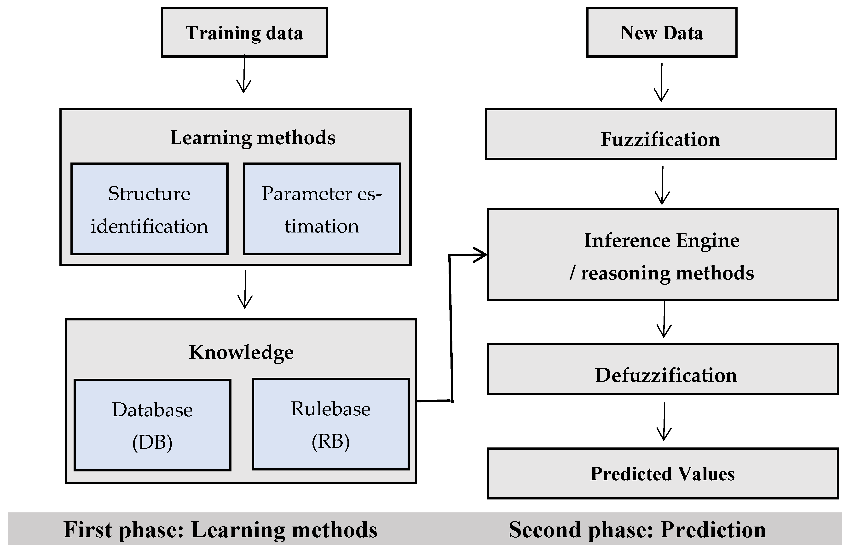
Figure 2 depicts the standard MM architecture, which consists of four components: fuzzification, a knowledge base, an inference engine, and a defuzzifier. The fuzzification interface transforms new input data into linguistic values in the second phase. The knowledge base includes a database and a rule base. The database contains fuzzy set definitions and membership function parameters, while the rule base provides collections of fuzzy IF–THEN rules. The inference engine performs reasoning operations on the appropriate fuzzy rules and input data. The defuzzifier generates crisp values from the linguistic values as a final result. Fuzzy rule-based systems (FRBS) are built using learning methods that extract information from data, which is divided into two steps: structure identification and parameter estimation. In the structure identification stage, a rule base that matches pairs of input and output variables is determined and the structure and number of rules are optimised. The parameter estimation process optimises the membership function parameters. The processing stages can be performed simultaneously or sequentially (Riza et al. 2015; Sugeno and Yasukawa 1993).
Kim and Kasabov (1999) proposed HyFIS as a learning method with a rule structure based on MM. The learning method consists of two phases: knowledge acquisition and structure and parameter learning. The knowledge acquisition module uses Wang and Mendel techniques. Structure and parameter learning is a supervised learning method that employs gradient-descent-based learning algorithms. The model created by the function comprises a rule database and membership function parameters. As a result, the mean and variance of the Gaussian function for both the antecedent and consequent parts are optimised.

3.3. FS.HGD Model

The Takagi–Sugeno–Kang (TSK) model differs from the MM in the IF–THEN rule by employing rules that represent the consequent parts as a function of input variables rather than dealing with linguistic variables (Sugeno and Kang 1988; Takagi and Sugeno 1985). FS.HGD is an FRBS function that utilizes heuristics and the gradient descent approach to implement a simplified TSK fuzzy-rule-generating method proposed by Ishibuchi et al. (1993). It is a special case within the TSK model and employs fuzzy rules with non-fuzzy singletons (i.e., real numbers) in the consequent part. The antecedent component of each rule is generated using space partitioning techniques, while the initial consequent part is generated using the weighted mean value of the training data. The value of the consequent part is then updated using the gradient descent method. The user’s heuristic value influences the weight of each data point.

3.3.1. Fuzzy System

The n-dimensional input and output spaces are assumed to be 0,1 n and [ 0,1 ] , respectively. A simple fuzzy grid based on triangular fuzzy sets is used to fuzzy partition the input space. Let x p = x p 1 , , x p m and y be input and output variables, respectively, where x ,   y R and R is the set of real numbers. The rule for the simplified fuzzy inference model is
Rule   i : IF   x 1   is   A i 1   and   x j   is   A i j   and   x m ,   THEN   y   is   ω i ,
where ( j = 1 , , m ) is a rule number, ( i = 1 , , n ) is a variable number, A i j is a membership function of the antecedent part ( x p 1 , , x p m ), and w i is a real number of the consequent part ( y ). A membership value of μ i of the antecedent part for input x is expressed as
μ i = j = 1 m A i j ( x j ) .
The output of fuzzy reasoning y can be derived from (8).
y = i = 1 n μ i ω i i = 1 n μ i .

3.3.2. Heuristic Method

Let m input–output pairs ( x p , y p ) ,   p = 1,2 , , m and the value of ω i of each fuzzy IF–THEN rule in (6) from the training data. The heuristic method is expressed as
ω j H M = p = 1 m μ j p y p p = 1 m μ j p ,     j = 1,2 , , N .
That is, ω j H M is the average of y p weighted by μ j p .
The main advantage of the heuristic method lies in its simplicity. This method is particularly useful when there is insufficient computation time to learn a specific task, as the value of ω j can be determined by (9) without any need for iterative learning procedures.

3.3.3. Learning Method

If there is sufficient computation time, learning methods may generate fuzzy IF–THEN rules with better performance than the heuristic method. In this subsection, we briefly describe a simple learning method based on the gradient descent method.
The total error for the p-th input–output pair ( x p , y p ) is defined as
E = p = 1 m E p = 1 2 p = 1 m { y ^ p y p } 2 .
The learning rule for ω j is derived from (8) and (10) with intersect 0.5 and the denominator in (8) equals 1 for any x p , such that
ω j n e w = ω j o l d + β ( E p ω j )
= ω j o l d β μ j p { y ^ p y p } , j = 1,2 , , N .
where β is the learning rate. The learning procedure is as follows:
  • Step 1: Specify the initial value ω j i n i t of ω j , the value of β and the maximum iteration number t m a x . Let t : = 0 .
  • Step 2: For p = 1,2 , , m , adjust each ω j by (8). Let t : = t   + 1.
  • Step 3: If t t m a x , then stop this procedure, else go to Step 2.
In computer simulations, the initial value ω j i n i t of ω j is specified in the following two ways:
4.
ω j i n i t = 0 ,   j = 1,2 , , N ,
5.
ω j i n i t = ω j H M ,   J = 1,2 , , N .

3.4. Accuracy Criteria

3.4.1. Algorithm of Self-Tuning

The objective function € estimates the inference error between the desired output and the output inferred through the self-tuning process. Let (p = 1, …, P) denote the number of input variables. The objective of learning is to minimise the mean square error (MSE):
M S E = 1 P P = 1 P ( y p y p r ) 2 .
To minimise the objective function MSE, each c, b, and w parameter is updated based on the learning rule expressed by the following formula:
z i ( t + 1 ) = z i ( t ) k ϑ M S E ϑ z i ,
where ( z i = c i j , b i j , w i j ), t is the number of iteration times, and k is the learning rate constant. The gradients of the objective function ϑ M S E ϑ z i in (13) can be derived from (14) to (16) as follows:
ϑ M S E ϑ z i = μ i i 1 n μ i ( y y r ) ,
ϑ M S E ϑ c i j = μ i i 1 n μ i ( y y r ) ( w i y ) x j c i j b i j 2 ,
ϑ M S E ϑ b i j = μ i i 1 n μ i ( y y r ) ( w i y ) ( x j c i j ) 2 b i j 3 .
Section 3.4.2 discusses the learning algorithm for the conventional fuzzy inference model.

3.4.2. Error Criteria Test

We evaluate the accuracy of our method using mean absolute percentage error (MAPE), mean error (ME), MAE, and root mean squared error (RMSE). The MAPE, also known as the mean absolute percentage deviation, is a statistical measure of prediction accuracy expressed as a percentage. It is defined as
M A P E = 1 n t = 1 n X t F t X t ,
where X t is the actual value, F t is the forecasted value, and n is the sample size. The absolute value in (14) is summed for every forecasted point in time and divided by the number of fitted points. MAE and ME are, respectively, defined as follows:
M A E = 1 n t = 1 n | X t F t | ,
M E = 1 n t = 1 n ( X t F t ) ,
The RMSE, also known as the root mean squared deviation, is a frequently used measure of the estimators’ differences. It measures the average error produced by the model in predicting the outcome of an observation. It is defined as
R M S E = M S E .

4. Data Description

This study utilized a comprehensive dataset of 2026 observations, consisting of day-to-day closing prices of the Tadawul stock market from August 2011 until December 2019. The closing prices are frequently used in technical analysis for predicting future trends and identifying trading opportunities. The study aims to provide valuable insights into the performance of the Saudi Arabian stock market, identify trends and patterns in its behaviour, and assist investors and financial analysts in making informed decisions about stock market investments in Saudi Arabia by analysing the Tadawul stock market’s closing prices.
Table 1 presents the statistical summary of three stocks in the Saudi Arabian stock market: LSCS, Repo, and Loil. The sample size for each stock is 2026, which ensures that the dataset is comprehensive and reliable for analysis. The table includes the mean, standard deviation, skewness, and kurtosis for each stock. The mean closing price provides information about the average price of each stock. LSCS has the highest mean at 6.749, followed by Loil at 4.299, and Repo has the lowest mean at 0.696. The standard deviation measures the dispersion of the data around the mean, with LSCS having the highest value at 0.692, followed by Loil at 0.354, and Repo having the lowest at 0.280. Skewness provides information about the symmetry of the distribution. LSCS has a negative skewness of −2.099, indicating that the distribution is skewed to the left, while Repo has a positive skewness of 2.006, indicating that the distribution is skewed to the right. Loil has a skewness of −0.175, which suggests that the distribution is approximately symmetric. Finally, the kurtosis statistic provides information about the shape of the distribution. LSCS has a kurtosis of 4.263, which means that the distribution is leptokurtic and has heavy tails. Repo has a kurtosis of 22.797, indicating that the distribution is extremely leptokurtic and has very heavy tails. Loil has a kurtosis of −1.107, indicating that the distribution is platykurtic and has light tails.

5. Empirical Results and Discussion

A hybrid model that combines the HyFIS, FS.HGD, and MODWT-LA8 models was proposed to predict Tadawul stock market closing prices from 2011 to 2019. The MODWT method uses WT such as Haar, d4, LA8, C6, and bl14. There are three steps in MODWT: decomposition, filtering, and reconstruction. In the decomposition step, the signal is divided into wavelet coefficients at different scales and positions. The filtering step extracts useful information from the signal by applying a filter bank to the wavelet coefficients. In the reconstruction step, the filtered wavelet coefficients are combined to obtain an approximation of the original signal. The MODWT categorises the data into two groups: detail series and approximation series, which are used when the original financial data have large fluctuations. We use an accuracy indicator to assess the model’s performance.
The proposed hybrid model is a novel method for predicting financial time series data. The methodology for this model involves four key steps. Firstly, the closing price data from Tadawul are collected as a basis for subsequent analysis. Secondly, the logarithmic standard deviation is used to calculate the LSCS, a metric that captures the level of volatility in the data. This is an important factor for forecasting. Thirdly, the LSCS data are decomposed using the MODWT function, which splits the data into two groups: low-fluctuating data (approximation coefficient) and high-fluctuating data (details coefficient). Finally, a robust approach is used to model the relationship between the LSCS and other financial variables, resulting in an accurate and reliable forecasting tool. The analysis uses five different MODWT functions (Haar, d4, LA8, C6, and bl14) with the approximation coefficient being the main feature used as an output in the forecasting model. The fourth step of the methodology involves applying the input variables and hybrid models to the LSCS approximation coefficient for each function, resulting in two proposed hybrid models, namely MODWT-HyFIS and MODWT-FS.HGD. These models use the LSCS approximation coefficient along with input variables (Loil and Repo) within HyFIS and FS.HGD.
A comparative study was then conducted between the best-performing models, MODWT-HyFIS and MODWT-FS.HGD, as well as alternative functions and traditional models (ARIMA, HyFIS, and FS.HGD). The proposed hybrid model offers an innovative approach to forecasting financial time series data by combining the strengths of the MODWT function, input variables, and hybrid models, resulting in a more accurate and reliable forecast than traditional methods. The comparative study highlights the superiority of the proposed models over alternative functions and traditional models, demonstrating the potential for this approach to be used in a range of financial forecasting applications. We used an 80/20 approach to analyse the suggested models, with 80% of the original data used for training the model and selecting the most effective one. The remaining 20% of the data were then used to test the performance of the selected model.

5.1. Selecting Variables

Table 2 shows the results of a multiple linear regression analysis of the relationship between input variables, Repo and Loil, and the output variable, LSCS, in the Saudi Arabian stock market. The table includes unstandardized coefficients, standardised coefficients (beta), t-values, and significance levels for the input variables, along with collinearity statistics such as tolerance and variance inflation factor (VIF) values. The analysis shows that both Repo and Loil have a significant impact on LSCS at the 0.01 level of significance. For every one-unit increase in Repo, LSCS increases by 0.198 units, holding all other variables constant. On the other hand, for every one-unit increase in Loil, LSCS decreases by 1.369 units, holding all other variables constant. The intercept, or constant, in the model is 12.495, indicating that LSCS would be predicted to be 12.495 when both Repo and Loil are equal to zero. The standardised coefficients show that a one-unit increase in Repo corresponds to a 0.080 standard deviation increase in LSCS, while a one-unit increase in Loil corresponds to a 0.699 standard deviation decrease in LSCS. The t-values for both input variables are significant, and the significance level for both input variables is less than 0.01, indicating that the results are highly statistically significant.
Collinearity statistics measure the correlation between input variables in a regression model. Tolerance and VIF are common measures of collinearity (Abinzano et al. 2023; Pallant 2020). Tolerance measures the variance in an input variable that is not explained by other variables, while VIF measures how much the variance of a regression coefficient is increased due to collinearity. The tolerance and VIF values for both input variables are acceptable, with tolerance values above 0.1 and VIF values less than 10. These values suggest that the variables do not share high collinearity, which could impact the model’s accuracy. Repo and Loil have the same tolerance and VIF values, indicating no collinearity between the two variables. The tolerance and VIF values for each variable are 0.893 and 1.120, respectively, indicating no significant multicollinearity in the model. Collinearity can lead to unstable estimates and reduced predictive power, so it is essential to check for it in regression analysis. The collinearity statistics presented in Table 2 ensure the model’s reliability and validity.

5.2. Results of FS.HGD and HyFIS

The output variable’s WT function for a dataset with an 80% coverage is shown in Table 3, which compares the performance of different WT functions with various ARIMA models. The results of the experiment were evaluated based on three error metrics: ME, MAE, and MAPE. The findings reveal that the LA-8 WT function with ARIMA(1,1,0) with drift provides the lowest ME of 0.000005320, while the Haar WT function with ARIMA(0,1,1) with drift yields the highest ME of 0.000396455. On the other hand, the BL-14 WT function with ARIMA(1,1,0) with drift provides the lowest MAE of 0.003294034, while the Haar WT function with ARIMA(0,1,1) with drift yields the highest MAE of 0.004708187. Finally, the LA-8 WT function with ARIMA(1,1,0) with drift also exhibits the lowest MAPE of 0.064496830, while the Haar WT function with ARIMA(0,1,1) with drift again produces the highest MAPE of 0.088929530.
In particular, the results suggest that the LA-8 WT function with ARIMA(1,1,0) with drift is the most suitable combination for this dataset, as it outperforms the other WT functions across all three error metrics. The LA-8 WT function has a longer filter length and a smoother response compared to the other wavelet functions, which may explain its superior performance. The ARIMA(1,1,0) model with drift takes into account both trend and frequency, which are crucial factors in time series forecasting. However, it is important to note that the performance of the WT functions and ARIMA models may vary depending on the specific characteristics of the dataset, such as data frequency and noise level.
Table 4 presents a comparative analysis of the WT functions with two models, FS.HGD and HyFIS, for forecasting a 20% dataset. The analysis was conducted based on three evaluation metrics, namely RMSE, MAE, and MAPE. Table 4 reports the performance of the FS.HGD and HyFIS models along with their performance when combined with different wavelet functions. In terms of RMSE, the best-performing model was MODWT-LA8-FS.HGD, with a score of 0.048. This was followed by MODWT-bl14-FS.HGD and MODWT-bl14-HyFIS with RMSE scores of 0.051 and 0.083, respectively. On the other hand, MODWT-LA8-HyFIS performed the worst, with an RMSE score of 0.605. For the MAE metric, MODWT-LA8-FS.HGD once again performed the best with a score of 0.038, followed by MODWT-bl14-FS.HGD with a score of 0.043. The worst performer was MODWT-LA8-HyFIS, with an MAE score of 0.423. In terms of MAPE, MODWT-LA8-FS.HGD was the best performer, with a score of 0.538. This was followed by MODWT-d4-FS.HGD and FS.HGD with MAPE scores of 0.648 and 1.092, respectively. The worst performer was MODWT-LA8-HyFIS, with a MAPE score of 6.794. In other words, it can be observed that the MODWT-LA8-FS.HGD model has the lowest RMSE and MAE values of 0.048 and 0.038, respectively. It also has the lowest MAPE value of 0.538, indicating the highest level of accuracy in predicting the values. On the other hand, the MODWT-LA8-HyFIS model has the highest RMSE and MAE values of 0.604 and 0.423, respectively, and the highest MAPE value of 6.794, indicating the lowest level of accuracy among all models.
Several aspects distinguish the current study from the previous study conducted by (Alshammari et al. 2023). Firstly, we propose two new hybrid models, namely HyFIS and FS.HGD, in conjunction with five functions of MODWT, whereas the previous study employed only the gradient descent learning (FIR.DM) model combined with MODWT. Secondly, our newly proposed hybrid models improve prediction accuracy compared to the previous model, as evidenced by their better RMSE and MAE values for predicting 20% of the datasets. Thirdly, both studies used the same dataset, period, and variables. Fourthly, while the approximate coefficients from MODWT for LSCS are the same in both articles, we identified a new hybrid model, MODWT-LA8-FS.HGD, which yields improved predictions for 20% of the datasets. The economic significance of this study can be seen in its potential to improve the accuracy of stock market prediction. Accurate predictions can lead to better investment decisions and ultimately improve the overall performance of the stock market. Additionally, the paper’s focus on the Saudi Arabian stock market provides insights into its performance and behaviour, which can be useful for investors and analysts in the region. Overall, the study’s hybrid models and methodology can contribute to the financial industry’s efforts to develop more reliable and efficient investment strategies.
Forecasting performance improves in some cases but decreases in others when the FS.HGD model is combined with various WT functions. For example, when combined with the d4, LA8, and bl14 WTs, the RMSE, MAE, and MAPE values decrease significantly. However, when combined with the Haar and C6 WTs, the values increase. The HyFIS model has an RMSE of 0.0860, MAE of 0.0816, and MAPE of 1.1504. When combined with various WT functions, the HyFIS model’s performance improves in some cases and deteriorates in others. For example, when combined with the bl14 WT, the RMSE and MAPE values decrease, but when combined with the LA8 WT, the values increase significantly. The results show that the combination of WT functions with the FS.HGD and HyFIS models can improve their performance in forecasting. However, the choice of WT function can have a significant impact on the accuracy of the models.

6. Limitations and Future Work

One limitation of this study is the limited number of input variables used to predict volatility. The study only considered oil price and repo rate as input variables. Though these are important macroeconomic variables in the Saudi Arabian context, using more variables could provide a more accurate prediction of volatility. Future research should consider including additional variables to improve the model’s predictive power. Another limitation is that the study only focused on the Tadawul stock exchange dataset. While this is a significant market, expanding the experiments to include data from other stock exchange markets, such as the New York Stock Exchange, National Association of Securities Dealers Automated Quotations, Shanghai Stock Exchange, and Hong Kong Stock Exchange, could provide a broader understanding of volatility prediction. This study only considered daily data from 2011 to 2019, which excludes the COVID-19 period. Considering the impact of the pandemic on financial markets and volatility, it is important to include COVID-19’s daily stock price data in future research to gain a better understanding of how the pandemic has affected volatility.

7. Conclusions

We presented valuable insights into the performance of the Saudi Arabian stock market by analysing the day-to-day closing prices of the Tadawul stock market from August 2011 until December 2019. The dataset of 2026 observations provides a reliable basis for analysis, and the statistical summary of LSCS, Repo, and Loil stocks in the Saudi Arabian stock market is presented in Table 1. The empirical results and discussion section proposes a hybrid model for predicting Tadawul stock market closing price data using the MODWT models combined with HyFIS and FS.HGD. The proposed hybrid models are a novel approach to forecasting financial time series data, and the methodology designed for these models includes four key steps: gathering closing price data, calculating LSCS, decomposing the LSCS data using the MODWT function, and applying input variables and hybrid models to the approximation coefficient. A comparative study was conducted between the best-performing models (MODWT-HyFIS, MODWT-FS.HGD) and alternative functions as well as traditional models (ARIMA, HyFIS, and FS.HGD). In the results, the oil price and the repo rate were selected as the input values in accordance with multicollinearity tests (tolerance and VIF) and multiple regressions. Repo and Loil have a significant impact on LSCS at the 0.01 level of significance. The collinearity statistics indicate that there is no significant multicollinearity between the variables, ensuring the reliability and validity of the regression model. The results also show that combining wavelet functions with the FS.HGD and HyFIS models can improve their predicting performance. The MODWT-LA8-FS.HGD model has the lowest RMSE and MAE values, which are 0.048 and 0.038, respectively. It also has the lowest MAPE value of 0.538, indicating the highest level of prediction accuracy. The proposed hybrid models can be valuable for investors and financial analysts in making informed decisions regarding stock market investments in Saudi Arabia. Overall, this article provides important insights into the performance of the Saudi Arabian stock market and identifies trends and patterns in the market’s behaviour. Overall, the hybrid models and methodology proposed in this study have practical implications for investors and financial analysts looking to make informed investment decisions in the stock markets. By providing more accurate predictions, the models can help investors avoid potential losses and maximize their returns. The insights into the behaviour and performance of the Saudi Arabian stock market can further inform investment decisions and contribute to the development of more efficient investment strategies.
However, there are still some policy implications that need to be considered for the sake of investors, traders, and policymakers. First, policymakers should focus on improving the transparency and reliability of the Saudi Arabian stock market. This can be achieved through implementing more stringent regulations and guidelines to ensure proper corporate governance and transparency in companies listed on the Saudi Arabian stock market. Second, policymakers should prioritize the development of more efficient investment strategies in the stock market by providing more resources and support for financial analysts and investors. This can include providing access to accurate and reliable data, promoting the use of new forecasting techniques, and encouraging the development of new financial models that can provide more accurate predictions for investors. Finally, investors and traders must also be aware of the risks associated with investing in the stock market, as well as the potential rewards. They must thoroughly research and analyse companies before making any investment decisions, as well as monitor the performance of the Saudi Arabian stock market regularly.

Author Contributions

Conceptualization, A.H.A., S.A.W. and J.J.J.; data curation, A.H.A., S.A.W. and J.J.J.; formal analysis, A.H.A. and J.J.J.; funding acquisition, J.J.J.; methodology, A.H.A., S.A.W. and J.J.J.; project administration, M.T.I., S.A.W. and J.J.J.; resources, M.T.I.; software, A.H.A. and J.J.J.; supervision, M.T.I., S.A.W. and J.J.J.; validation, M.T.I., S.A.W. and J.J.J.; visualization, A.H.A. and J.J.J.; writing—original draft, A.H.A. and J.J.J.; writing—review and editing, M.T.I. and J.J.J. All authors have read and agreed to the published version of the manuscript.

Funding

This research was funded by the University of Ha’il (Ref. 41/4/34452).

Data Availability Statement

The databases utilized to support the conclusions of this study are obtainable upon request from the corresponding author.

Acknowledgments

The authors would like to express their sincere appreciation for the financial assistance provided to them by the University of Ha’il (Ref. 41/4/34452) to complete this study.

Conflicts of Interest

The authors declare no conflict of interest.

References

  1. Abinzano, Isabel, Harold Bonilla, and Luis Muga. 2023. Duty calls: Prediction of failure in reorganization processes. The Journal of Risk Finance 24: 337–53. [Google Scholar] [CrossRef]
  2. Adil, Iftikhar H. 2015. A modified approach for detection of outliers. Pakistan Journal of Statistics and Operation Research XI: 91–102. [Google Scholar] [CrossRef] [Green Version]
  3. Al Rahahleh, Naseem, and Robert J. Kao. 2018. Forecasting volatility: Evidence from the Saudi stock market. Journal of Risk Financial Management 11: 84. [Google Scholar] [CrossRef] [Green Version]
  4. Alenezy, Abdullah H., Mohd Tahir Ismail, Jamil J. S. Jaber, AL Wadi, and Rami S. Alkhawaldeh. 2022. Hybrid fuzzy inference rules of descent method and wavelet function for volatility forecasting. PLoS ONE 17: e0278835. [Google Scholar] [CrossRef] [PubMed]
  5. Alkhatib, Khalid, Mothanna Almahmood, Omar Elayan, and Laith Abualigah. 2022. Regional analytics and forecasting for most affected stock markets: The case of GCC stock markets during COVID-19 pandemic. International Journal of System Assurance Engineering and Management 13: 1298–308. [Google Scholar] [CrossRef]
  6. Alqahtani, Abdullah, Elie Bouri, and Xuan Vinh Vo. 2020. Predictability of GCC stock returns: The role of geopolitical risk and crude oil returns. Economic Analysis and Policy 68: 239–49. [Google Scholar] [CrossRef]
  7. Alshammari, Tariq T., Mohd T. Ismail, Nawaf N. Hamadneh, S. Al Wadi, and Jamil J. Jaber. 2023. Forecasting Stock Volatility Using Wavelet-based Exponential Generalized Autoregressive Conditional Heteroscedasticity Methods. Intelligent Automation Soft Computing 35: 2589–601. [Google Scholar] [CrossRef]
  8. Al-Wadi, S., Osama M. Al-Rawashdeh, Omar ALsinglawi, Bara’ah A. ABU Dalwein, and Jamil J. Jaber. 2022. Revenue’s Forecasting of Aqaba Ports Company Using Wavelet Transform and ARIMA Models. PRZESTRZEN 22: 143–60. [Google Scholar]
  9. Aseeri, Ahmad O. 2023. Effective short-term forecasts of Saudi stock price trends using technical indicators and large-scale multivariate time series. PeerJ Computer Science 9: e1205. [Google Scholar] [CrossRef]
  10. Bhagat, Surah K., Tiyasha Tiyasha, Zainah Al-Khafaji, Patrick Laux, and Ahmed A. Ewees. 2022. Establishment of dynamic evolving neural-fuzzy inference system model for natural air temperature prediction. Complexity 2022: 1047309. [Google Scholar] [CrossRef]
  11. Bollerslev, Tim. 1986. Generalized autoregressive conditional heteroskedasticity. Journal of Econometrics 31: 307–27, Reprinted in Journal of Econometrics 234: 25–37. [Google Scholar] [CrossRef] [Green Version]
  12. Bouri, Elie, Rami Hammoud, and Christina Abou Kassm. 2023. The effect of oil implied volatility and geopolitical risk on GCC stock sectors under various market conditions. Energy Economics 120: 106617. [Google Scholar] [CrossRef]
  13. Ciner, Cetin. 2019. Do industry returns predict the stock market? A reprise using the random forest. The Quarterly Review of Economics Finance 72: 152–58. [Google Scholar] [CrossRef]
  14. Dai, Zhifeng, and Haoyang Zhu. 2023. Dynamic risk spillover among crude oil, economic policy uncertainty and Chinese financial sectors. International Review of Economics and Finance 83: 421–50. [Google Scholar] [CrossRef]
  15. Dai, Zhifeng, Haoyang Zhu, and Xinhua Zhang. 2022. Dynamic spillover effects and portfolio strategies between crude oil, gold and Chinese stock markets related to new energy vehicle. International Review of Financial Analysis 109: 105959. [Google Scholar] [CrossRef]
  16. Engle, Robert F. 1982. Autoregressive Conditional Heteroscedasticity with Estimates of the Variance of United Kingdom Inflation. Econometrica: Journal of the econometric society 50: 987–1007. [Google Scholar] [CrossRef]
  17. Ishibuchi, Hisao, Ken Nozaki, Hideo Tanaka, Yukio Hosaka, and Masanori Matsuda. 1993. Empirical study on learning in fuzzy systems. Paper presented at Second IEEE International Conference on Fuzzy Systems, San Francisco, CA, USA, March 28–April 1; pp. 606–11. [Google Scholar]
  18. Jaber, Jamil J., Noriszura Ismail, S. Al Wadi, and Mohammad H. Saleh. 2017. Forecasting of volatility risk for Jordanian banking sector. Far East Journal of Mathematical Sciences 101: 1491–507. [Google Scholar] [CrossRef]
  19. Jaber, Jamil J., Rami S. Alkhawaldeh, Samar M. Alkhawaldeh, Raed Masa’adeh, and Muhammad T. Alshurideh. 2023. Predicting Bitcoin Prices Using ANFIS and Haar Model. In The Effect of Information Technology on Business and Marketing Intelligence Systems. Berlin: Springer, pp. 2421–36. [Google Scholar]
  20. Jozi, Aria, Tiago Pinto, Isabel Praça, Francisco Silva, and Brigida Teixeira. 2016. Energy consumption forecasting based on hybrid neural fuzzy inference system. Paper presented at 2016 IEEE Symposium Series on Computational Intelligence (SSCI), Athens, Greece, December 6–9; pp. 1–5. [Google Scholar]
  21. Kim, Jaesoo, and Nikola Kasabov. 1999. HyFIS: Adaptive neuro-fuzzy inference systems and their application to nonlinear dynamical systems. Neural Networks 12: 1301–19. [Google Scholar] [CrossRef]
  22. Mamdani, Ebrahim H. 1974. Application of fuzzy algorithms for control of simple dynamic plant. IET Proceedings of the Institution of Electrical Engineers 121: 1585–88. [Google Scholar] [CrossRef]
  23. Mamdani, Ebrahim H., and Sedrak Assilian. 1975. An experiment in linguistic synthesis with a fuzzy logic controller. International Journal of Man-Machine Studies 7: 1–13. [Google Scholar] [CrossRef]
  24. McBratney, Alex B., Budiman Minasny, and Uta Stockmann. 2018. Pedometrics. Berlin: Springer. [Google Scholar]
  25. Pallant, Julie. 2020. SPSS Survival Manual: Step by Step Guide to Data Analysis Using IBM SPSS. London: Routledge. [Google Scholar]
  26. Patel, Jigar, Sahil Shah, Priyank Thakkar, and Ketan Kotecha. 2015a. Predicting stock and stock price index movement using trend deterministic data preparation and machine learning techniques. Expert Systems with Applications 42: 259–68. [Google Scholar] [CrossRef]
  27. Patel, Jigar, Sahil Shah, Priyank Thakkar, and Ketan Kotecha. 2015b. Predicting stock market index using fusion of machine learning techniques. Expert Systems with Applications 42: 2162–72. [Google Scholar] [CrossRef]
  28. Riza, Lala S., Christoph N. Bergmeir, Herrera Triguero, and Sánchez J. M. Benítez. 2015. FRBS: Fuzzy Rule-Based Systems for Classification and Regression in R. Boston: American Statistical Association. [Google Scholar]
  29. Sayed, Omer A., and Hussein Eledum. 2021. The short-run response of Saudi Arabia stock market to the outbreak of COVID-19 pandemic: An event-study methodology. International Journal of Finance Economics 26: 4857–6487. [Google Scholar] [CrossRef]
  30. Silva, Francisco, Brigida Teixeira, Nuno Teixeira, Tiago Pinto, and Isabel Praça. 2016. Application of a hybrid neural fuzzy inference system to forecast solar intensity. Paper presented at IEEE 27th International Workshop on Database and Expert Systems Applications (DEXA), Porto, Portugal, September 5–8; pp. 161–65. [Google Scholar]
  31. Sugeno, Michio, and Geuntaek Kang. 1988. Structure identification of fuzzy model. Fuzzy Sets Systems 28: 15–33. [Google Scholar] [CrossRef]
  32. Sugeno, Michio, and Takahiro Yasukawa. 1993. A fuzzy-logic-based approach to qualitative modeling. IEEE Transactions on Fuzzy Systems 1: 7. [Google Scholar] [CrossRef] [Green Version]
  33. Takagi, Tomohiro, and Michio Sugeno. 1985. Fuzzy identification of systems and its applications to modeling and control. IEEE Transactions on Systems, Man, Cybernetics 1: 116–32. [Google Scholar] [CrossRef]
  34. Tien, Ho Thuy, and Ngo Thai Hung. 2022. Volatility spillover effects between oil and GCC stock markets: A wavelet-based asymmetric dynamic conditional correlation approach. International Journal of Islamic and Middle Eastern Finance and Management 15: 1127–49. [Google Scholar] [CrossRef]
  35. WFE. 2020. WFE Annual Statistics Guide 2020. Available online: https://www.world-exchanges.org/our-work/articles/2020-annual-statistics-guide (accessed on 1 January 2020).
  36. Yaacob, Nurul A., Jamil J. Jaber, Dharini Pathmanathan, Sadam Alwadi, and Ibrahim J. Mohamed. 2021. Hybrid of the Lee-Carter model with maximum overlap discrete wavelet transform filters in forecasting mortality rates. Mathematics 9: 2295. [Google Scholar] [CrossRef]
  37. Zadeh, Lotfi A. 1975. Calculus of fuzzy restrictions. In Fuzzy Sets and Their Applications to Cognitive and Decision Processes. Amsterdam: Elsevier, pp. 1–39. [Google Scholar]
  38. Zhang, Guoqiang, Eddy B. Patuwo, and Michael Y. Hu. 1998. Forecasting with artificial neural networks: The state of the art. International Journal of Forecasting 14: 35–62. [Google Scholar] [CrossRef]
  39. Ziadat, Salem Adel, and David G. McMillan. 2022. Oil-stock nexus: The role of oil shocks for GCC markets. Studies in Economics and Finance 39: 801–18. [Google Scholar] [CrossRef]
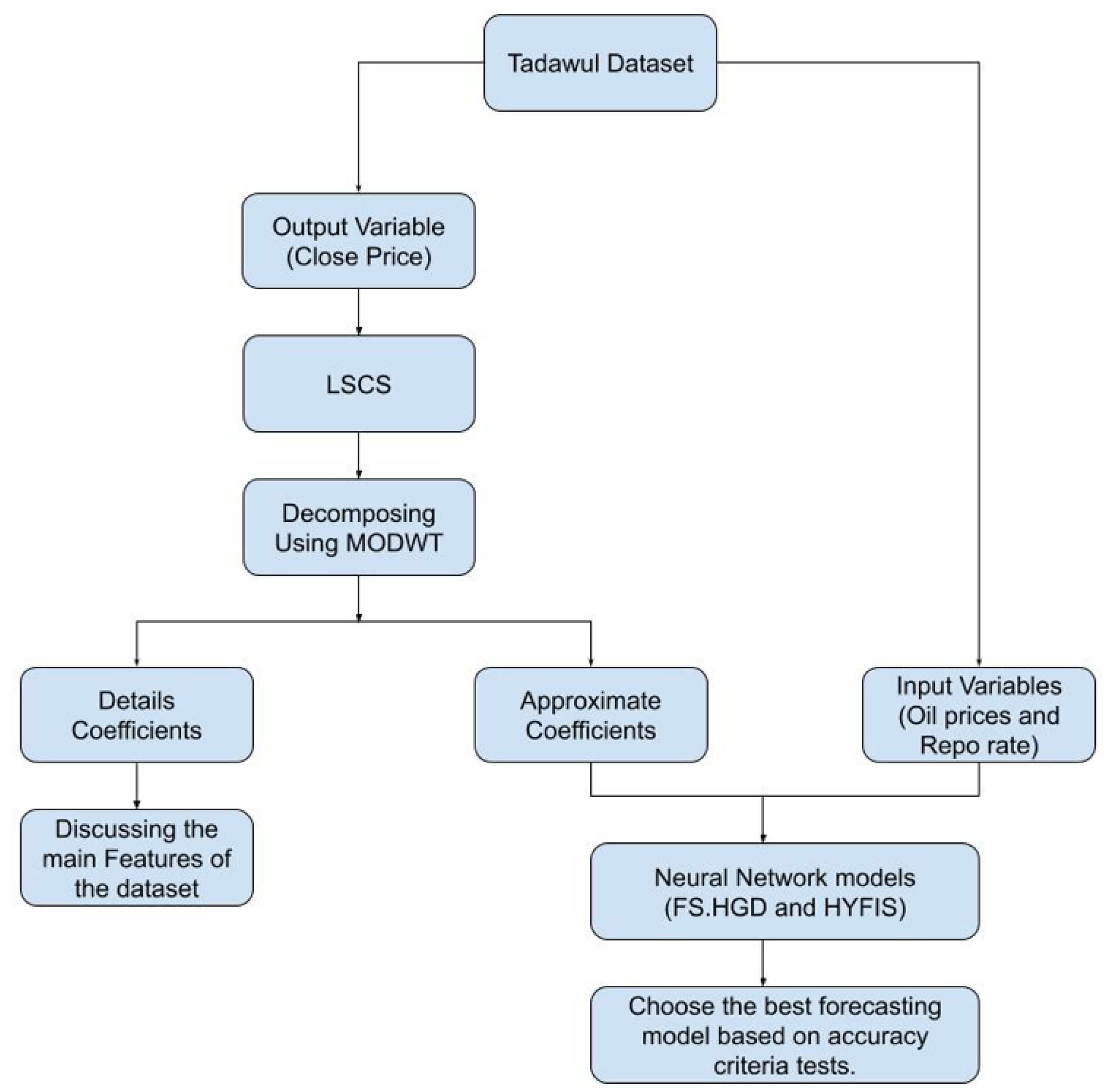
Figure 1. The flowchart of MODWT with FS.HGD and HYFIS.
Risks 11 00121 g001
Figure 2. Learning and prediction phase of an FRBS and Mamdani model.
Risks 11 00121 g002
Table 1. A statistical summary of LSCS, Repo, and Loil in the Saudi Arabian stock market.
LSCSRepoLoil
Sample size202620262026
Arithmetic mean6.749 0.696 4.299
Standard deviation0.692 0.280 0.354
Skewness−2.099 2.006 −0.175
Kurtosis4.263 22.797 −1.107
Table 2. Multiple linear regression analysis for LSCS in the Saudi Arabian stock market.
VariablesUnstandardized CoefficientsStandardized CoefficientstSig.Collinearity Statistics
BStd. ErrorBetaToleranceVIF
(Constant)12.4950.139 89.6340.000
Repo0.1980.0430.0804.6210.0000.8931.120
Loil−1.3690.034−0.699−40.3550.0000.8931.120
Table 3. Comparative analysis of WT functions for time series forecasting on 80% dataset.
WT FunctionMEMAEMAPE
HaarARIMA(0,1,1) with drift0.0003964550.0041306760.08892953
Db4ARIMA(0,1,0)0.0005756730.0047081870.09547983
LA-8ARIMA(1,1,0)0.000005320.0032141820.06449683
BL-14ARIMA(1,1,0) with drift0.0000095640.0032940340.06557786
C6ARIMA (1,1,0) with drift0.0000329950.0033146550.06604977
Table 4. Comparative analysis of WT functions with FS.HGD and HyFIS models on 20% dataset.
ModelsRMSEMAEMAPE
FS.HGD0.1056361850.0764414811.092438331
MODWT-Haar-FS.HGD0.1290522140.0936890451.347518627
MODWT-d4-FS.HGD0.0586614440.0463394640.648079708
MODWT-LA8-FS.HGD0.0482603120.0384418290.538406565
MODWT-bl14-FS.HGD0.0509001520.0426389410.597125838
MODWT-C6-FS.HGD0.08292420.0756601661.055475213
FS.HGD+ARIMA direct0.0850569960.0753597051.050702605
HyFIS0.0860247020.0815979591.150437522
MODWT-Haar-HyFIS0.0921974580.0857093261.198456099
MODWT-d4-HyFIS0.0906898130.0841321961.177323058
MODWT-LA8-HyFIS0.6048944680.4230328496.794333688
MODWT-bl14-HyFIS0.0828878340.0713523580.995263056
MODWT-C6-HyFIS0.0912497450.0834649191.165024215
HyFIS+ARIMA direct0.0860247020.0815979591.150437522
Disclaimer/Publisher’s Note: The statements, opinions and data contained in all publications are solely those of the individual author(s) and contributor(s) and not of MDPI and/or the editor(s). MDPI and/or the editor(s) disclaim responsibility for any injury to people or property resulting from any ideas, methods, instructions or products referred to in the content.