Abstract
We present a method for the arbitrage-free interpolation of plain-vanilla option prices and implied volatilities, which is based on a system of integral equations that relates terminal density and option prices. Using a discretization of the terminal density, we write these integral equations as a system of linear equations. We show that the kernel matrix of this system is, in general, ill-conditioned, so that it cannot be solved for the discretized density using a naive approach. Instead, we construct a sparse model for the kernel matrix using singular value decomposition (SVD), which allows us not only to systematically improve the condition number of the kernel matrix, but also determines the computational effort and accuracy of our method. In order to allow for the treatment of realistic inputs that may contain arbitrage, we reformulate the system of linear equations as an optimization problem, in which the SVD-transformed density minimizes the error between the input prices and the arbitrage-free prices generated by our method. To further stabilize the method in the presence of noisy input prices or arbitrage, we apply an -regularization to the SVD-transformed density. Our approach, which is inspired by recent progress in theoretical physics, offers a flexible and efficient framework for the arbitrage-free interpolation of plain-vanilla option prices and implied volatilities, without the need to explicitly specify a stochastic process, expansion basis functions or any other kind of model. We demonstrate the capabilities of our method in a number of artificial and realistic test cases.
1. Introduction
Since the dawn of modern quantitative finance, academics and practitioners have tried to understand the dynamics of asset price fluctuations, which, in financial markets, are called volatility. Understanding volatility is not only necessary for the risk management of financial products in general, but also, specifically, for the pricing of option contracts, since their value depends on the size of expected price fluctuations for the respective underlying assets. These studies have produced various books and reviews (Carr and Lee 2009; Clark 2010; Derman and Miller 2016; Gatheral 2006), as well as many focused studies for which we can cite only a few examples here: (Aït-Sahalia et al. 2001; Baker et al. 2004; Egloff et al. 2010; Hagan et al. 2001; Jiang 2020; Lipton 2002; Mixon 2002; Xing et al. 2010). Over time, many option pricing models have emerged, which assume specific dynamics for the underlying asset and its volatility. Among them are the seminal Black and Scholes (1973) model and the, similarly influential, Heston (1993) model, which specify an explicit stochastic process for the price of the underlying asset, and also for the volatility, in the case of the Heston model.
Most option pricing models require knowledge of various parameters which reflect the state of the market, such as interest rate, dividends or implied volatilities. If, for example, the ubiquitous Black–Scholes model (Black and Scholes 1973) is applied to realistic settings, it requires an implied volatility for each strike for which a price is intended. This implied volatility characterizes the size of price fluctuations for the option’s underlying asset, which is implied by the price of the option, i.e., only when this value of volatility is inserted into the pricing formula does one obtain the same price as is observed on the market.
Plain-vanilla European options for many underlyings are traded on exchanges, but for a fixed discrete set of strikes. To price a plain-vanilla option with a strike not contained in this set of market-quoted instruments, it is necessary to calculate the volatility for this missing strike out of the available option prices. Often, this is done not only by implying the volatility for single strikes, but by constructing a continuous representation of the implied volatility out of the discrete set of quoted option prices. Other use cases for such a continuous representation of implied volatility include the construction of a local volatility (LV) (Derman and Kani 1994; Dupire 1994) for use in the popular class of local stochastic volatility (LSV) models (Lipton 2002; Lipton et al. 2014), or the pricing of exotic derivatives. (Carr and Lee 2009).
There are many methods for constructing a continuous representation of option prices or implied volatilities, starting from simple spline interpolation, directly applied to the implied volatility, and moving to sophisticated arbitrage-free schemes in either volatility or option prices. Kahale (2004) uses a interpolating function to produce an arbitrage-free interpolation of option prices, but requires that the inputs also be arbitrage-free. Andreasen and Huge (2011) developed a one-step finite difference scheme to calibrate a piecewise constant local volatility model to quoted option prices. Jäckel (2014) formulates another method to construct interpolants for option prices and presents an algorithm to remove arbitrage from these interpolants. Another approach, developed by Le Floc’h and Osterlee (2019a, 2019b) directly relates option prices and terminal density using stochastic collocation to various basis functions. Such a relation exists, since the fair price of any financial instrument is the present value of its expected payoff. This expected payoff can be calculated from the payoff function of the instrument and the risk-neutral probability distribution. For plain-vanilla options, which are investigated herein, the payoff is only determined at maturity, so that the terminal density is sufficient to calculate the expected payoff (Breeden and Litzenberger 1978).
A totally different route to a continuous representation of option prices or implied volatility are stochastic volatility models, such as the Heston (1993), or SABR (Hagan et al. 2015) models and related approximate formulae for the volatility smile (Gatheral and Jacquier 2014; Lorig et al. 2017). These models are usually based on, or inspired by, a stochastic process with few parameters. Therefore, the forms of the volatility smiles in these models are somewhat inflexible, and it can be hard to fit them to market-quoted prices. Nevertheless, these models describe the whole dynamics of an underlying asset, instead of just the terminal density at a given point in time, which enables them to also price path-dependent options (Carr et al. 2022; Guterding and Boenkost 2018; Tian et al. 2014) and other exotic derivatives. (Guterding 2021; Zhu and Lian 2012).
Our aim here was to find a method for which it is not necessary to specify a stochastic process and which should also not require specifying a specific functional form for either the volatility or the terminal density. Such a method for the interpolation of implied volatilities would be versatile and applicable to a broad range of realistic situations. Inspired by recent progress on inverse problems in theoretical physics (Otsuki et al. 2020), we present a new method that uses the singular value decomposition (SVD) and -regularization to obtain a sparse model, i.e., one containing only a few non-zero parameters of the relation between plain-vanilla European option prices and the terminal density of the underlying asset. Using a constrained and -regularized optimization, our method is able to extract arbitrage-free representations of both option prices and implied volatilities, even from inputs that contain severe arbitrage, without any de-arbitraging or pre-processing steps. Since we are directly working with the density, our method is also able to extrapolate implied volatilites in an arbitrage-free manner beyond the quoted strike range.
We first review the relation between option prices and terminal density and describe how it can be discretized and written in matrix form. We show why naive attempts to invert this system of equations fail, in general, and propose a solution that involves transforming the problem into a better-conditioned one using the SVD. Then, we reformulate the procedure for finding the terminal density from a matrix inversion into a constrained optimization problem that also avoids arbitrage. We test our method on several classic examples, such as normal and log-normal densities. Furthermore, we show that our method can easily handle multimodal densities, arbitrage and volatility smiles with kinks, all of these being areas in which stochastic volatility models struggle (Le Floc’h and Osterlee 2019a). We conclude with a summary of the advantages and disadvantages of our method.
2. Methodology
2.1. Relation between Terminal Density and Option Price
Suppose we know the probability distribution or density for the price of an asset at time T. Then, we may calculate the price of a European option on this underlying asset at time t, with strike K and expiry at time T, from the following integral: (Breeden and Litzenberger 1978)
The time to expiry is given by and r is a risk-free interest rate. The kernel depends on the type of option we want to price. For a European Call option we use the following kernel:
For a European Put option we use another kernel:
In cases when the price of the underlying asset is, for example, non-negative, such as a stock, or obeys some other restriction, this may be taken into account not only by picking a suitable probability distribution , but also by adjusting the integral boundaries.
For numerical calculations, it is useful to discretize . If we pick a relevant interval , divide it into L, not necessarily uniform, sub-intervals and apply the trapezoidal rule, we obtain a discrete representation of Equation (1). Using the abbreviation , it reads:
If we pick a uniform discretization of the interval , we obtain the following simplified approximation:
As we refine the interval into smaller sub-intervals, the calculated price converges to the true price.
2.2. Matrix Representation of the Relation between Option Price and Terminal Density
From Equation (1), it is clear that the same density, , should be used for Call and Put options with the same underlying and expiry at T. Different strikes are taken into account through the kernel . In practice, European Call and Put options are often traded on exchanges, such that quoted prices for a set of discrete strikes are publicly available.
Based on these prices, we would like to find an approximation to the density . We write down a matrix equation that relates all M available Call and Put prices to the uniformly discretized density with N points (see Equation (5)):
Here, we absorbed into the function . If the option with index i is a Call option with strike , we use:
If the option with index i is a Put option, we use:
2.3. The Difficulty in Implying the Terminal Density from Option Prices
In general, we are interested in a finely resolved density with N discrete points in the interval , while only a limited number of option prices M is available. Hence, G in Equation (6) is, in general, not a square, but an matrix, where and often even . Therefore, G is ill-conditioned and cannot, in general, be inverted to find the vector of on the right-hand side.
A way to circumvent this difficulty is provided by the singular value decomposition (SVD) of a matrix. The singular value decomposition of G reads:
Here, T denotes the transpose of a matrix. Matrices U and V are orthogonal matrices of sizes and . S is a matrix of size , which contains, on its diagonal, the singular values , where . The singular values are non-negative real numbers in descending order.
This means we can write Equation (6) as:
Since U and V are orthogonal matrices (), we can multiply from the left by and obtain:
We now introduce the abbreviations and , which we call transformed quantities from now on. Prices are the SVD-transformed prices, while is the SVD-transformed density. With these transformed quantities we can write Equation (11) in the following form:
Since the matrix of singular values S in Equation (12) is diagonal, we conclude that an element-wise equation also holds:
This shows that the transformation from to Pr via G can be decomposed into three steps:
- application of a basis transformation from to via
- weighting the elements of with the singular values S to get via
- application of a basis transformation from to Pr via
Whether such a transformation is easily invertible, is characterized by the decay of singular values and, in particular, by the condition number . While the best-conditioned system of equations has , we are dealing here with the kernel matrix G (see Equation (6)), for which .
To show this, we analyze the kernel G for an equidistant discretization of the interval with 10,000 points and a variable number of strikes in the same interval. For simplicity, we only take into account Call options. The condition number as a function of the number of option strikes M in the problem is shown in Figure 1.
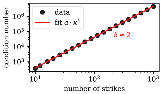
Figure 1.
Log–log plot of the condition number of the kernel matrix G defined in Equation (6) as a function of the number of strikes. The fit with clearly shows that the growth of the condition number follows such a power law with exponent .
We fit the condition number of the matrix G with a power law of the form , where we take x to be the number of option strikes. The fit clearly reveals that , which means that the condition number increases quadratically with the number of options taken into account. Importantly, even if only as few as ten strikes are considered, we already have , i.e., the system is very ill-conditioned and any naive attempt at solving Equation (6) for will not succeed.
2.4. Rapid Decay of the Kernel Matrix Singular Values
The fact that G is, in general, ill-conditioned leads to problems in treating Equation (6) numerically. In the previous section, we discussed how the condition number increases rapidly as we consider a larger number of options. This indicates that the additional singular values associated with additional market quotes, i.e., additional linear equations, decay rapidly.
Here, we show that the singular values also decay rapidly for a fixed matrix G, i.e., for a fixed number of considered options M and for a fixed number of discretization points N within . We chose equidistant strikes in a fixed interval and varied the number of discretization points N. As before, we only took into account Call options. The normalized singular values are shown in Figure 2. We attempted to fit the decay of singular values with an inverse power law of the form . The initial decay seemed to follow such a law with roughly and slowed down a little for the tail of singular values.
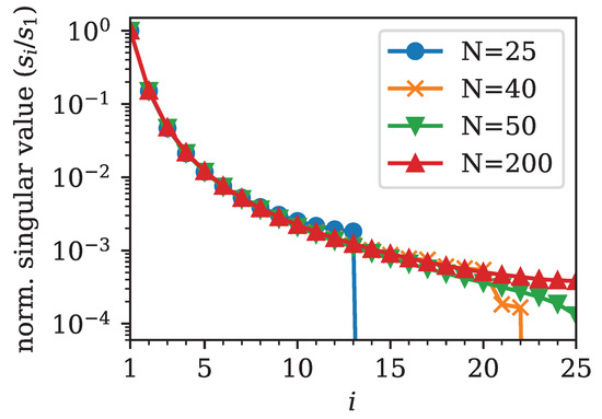
Figure 2.
Logarithmic plot of the normalized singular values for various numbers of discretization points N. The number of strikes is fixed to . The normalized singular values decay with an inverse power law of the form with .
Recall from the previous section (see Equation (13)) that the singular values play the role of weights for the transformed density to obtain the transformed prices . From Figure 2, it is obvious that these weights may differ by several orders of magnitude.
In any direct inversion method this would cause severe numerical problems, essentially because we would calculate , wherein we would have to divide by the quickly decaying singular values .
However, the role of as weights also shows that most of the relevant information must be contained in the first few basis vectors associated with the largest singular values. Therefore, we may consider only a limited number of these singular values and basis vectors to reconstitute a better-conditioned approximate version of G.
Let us fix the number of considered singular values to Q, where . We take the Q largest singular values and form the new diagonal matrix . We also reduce the dimensionality of U with to with and of with to with , by keeping only the first Q columns for or rows for , respectively. Thus, the new kernel matrix reads:
The matrix is still of size , but is better conditioned than the initial matrix G, which it aims to approximate. We achieved this by cutting off the tail of singular values with , for which we know that . Thus, the condition number of is , for which we know, in general, that . However, since we have already shown that singular values for our kernel matrix G decay with a power law (see Figure 2), we can safely assume that if the chosen Q is sufficiently small, i.e., the tail of small singular values is discarded.
This means we can systematically reduce the condition number of our kernel to obtain a better-conditioned kernel matrix by retaining only the largest singular values and associated orthogonal vectors, which is accomplished by lowering Q.
The prices Pr and the density are now related by the new kernel matrix , which gives us a new relation similar to Equation (10):
How good the approximation of G by is, obviously depends on how many singular values we retain, i.e., how we pick Q.
We also note that Pr and have M and N entries, respectively, while the transformed quantities and both only have Q entries. Since we are often interested in cases where , this can make a large difference computationally.
In this sense, the SVD allows us to describe the relation between density and prices with only a few parameters and related orthogonal vectors. Therefore, we may say that the SVD gives us a sparse model of the original relation defined by Equation (6).
This, however, does not mean that our method is only useful for sparse inputs. Rather, our method generates a sparse representation of the relation between any number of input prices and any number of density discretization points.
2.5. Optimization Problem for Finding the Density
So far, we have discussed how to treat the kernel matrix G of Equation (6) that relates prices Pr and densities . Remember that, in practice, the prices Pr are known, and, thus, we are interested in the density . This means we now attempt to solve Equation (6) approximately, by actually solving Equation (15).
This could work in cases in which the input prices are reachable with a non-negative density, i.e., they contain no arbitrage. In many other methods this is solved by filtering the input prices or applying some other form of de-arbitraging. (Jäckel 2014; Kahale 2004; Le Floc’h and Osterlee 2019a).
However, we can resolve the need for de-arbitraging by reformulating Equation (15) in the form of a constrained optimization problem. This optimization problem should give us the non-negative density with N entries. In our sparse model, is, however, directly related to , which has only Q entries. Therefore, the most efficient way to find is to actually find via optimization.
To this end, we minimize the squared error in the transformed quantities:
To further enhance the sparsity in the transformed domain, we add another term for -regularization with a free parameter :
The same optimization may also be carried out based on the deviation from the non-transformed prices Pr:
We still cannot guarantee that the density is non-negative, as it should be. Therefore, we constrain the optimization with the following additional conditions:
Furthermore, the integral of the density, expressed using the trapezoidal rule as before, should be equal to one:
Our goal is now to find the transformed density that minimizes Equation (18) under the constraints defined by Equations (19) and (20). The true density can then be calculated from the solution of the optimization problem via .
In Appendix A we discuss further details of how to calculate the error in prices and when it may be reasonable to convert between Call and Put prices.
In cases in which not only the mid-price is known, but also the Bid–Ask spread for each option is known, one could reformulate the optimization problem in Equation (18) to penalize calculated prices that lie outside the spread. We leave this problem for further studies.
2.6. Finding a Solution to the Optimization Problem
We implemented the system of equations defined by Equation (18) under the constraints defined by Equations (19) and (20) using the domain-specific language CVXPY (Agrawal et al. 2018; Diamond and Boyd 2016), available as a package for the Python programming language.
The transformed density that minimizes the squared error with additional -regularization on (see Equation (18)) can be found using various optimization algorithms. While some authors recommend using their own implementation of the Alternating Direction Method of Multipliers (ADMM) (Boyd et al. 2010), we have found that the open-source solvers ECOS (Domahidi et al. 2013) and SCS (O’Donoghue et al. 2016) both deliver excellent performances, especially with systems, such as the system we attempt to solve, which usually have only a few degrees of freedom (remember that has only Q entries). Therefore, we refer readers who are interested in details of the implementation of these solvers to the respective papers. In our case, ECOS seemed to be a good choice for the numerical solver.
For further considerations on how to efficiently solve the optimization problem, please see Appendix B. For readers interested in the computer code of our reference implementation, we provide a full working example on Github.1
2.7. A Measure for the Similarity of Probability Distributions
For test cases with known probability distributions we wanted to quantify the degree to which our method recovered the known density. A suitable measure for the similarity of probability distributions is the Bhattacharyya (1943) distance , which, for two probability distributions, and , is defined as:
If the probability distributions and are identical, i.e., the overlap is maximal, the integral under the logarithm is equal to one and the Bhattacharyya distance is zero. For all other cases, the overlap calculated from the integral is between zero and one, or exactly zero when there is no overlap. The Bhattacharyya distance is a non-negative number which approaches in cases where there are no overlaps.
In practice, we sample the probability distributions that are exactly known on the same grid for which we know our implied density and calculate the integral in Equation (21), using the trapezoidal rule.
3. Examples
In this section, we calculate option prices for a number of known densities and show that our method is able to accurately recover the terminal density only using the supplied prices. Furthermore, we demonstrate that our method is able to reconstruct densities from realistic input prices without any de-arbitraging, filtering or other pre-processing steps.
Since our implied density is non-negative, we can safely apply linear interpolation to the density and calculate option prices with strikes between the available input prices. This enables us to also interpolate implied volatilities by calculating these from the interpolated option prices.
3.1. Normal Density
A normal density corresponds to the Bachelier model, which, having mostly been ignored for a long time, has regained attention in the context of negative interest rates and negative prices for oil-futures. (Bachelier 1901; Choi et al. 2022).
Using the forward price F of the underlying asset, the strike of the option K, the normal volatility and the time to expiry , we define the moneyness m of an option in the following way:
Denoting the normal density function as and the cumulative normal density function as , the pricing formula of the Bachelier model can be expressed as follows for a Call option:
For the Put option it reads:
We fixed the initial underlying price to , the normal volatility to , the interest rate to and the time to expiry to . We then calculated the prices of 200 Call and Put options for a uniformly discretized grid of strikes between and .
We used our method with the option prices so-calculated to imply the density on a uniformly discretized grid with , and . We retained singular values.
The normal distribution, upon which the Bachelier model is based, was recovered to a high degree of accuracy (see Figure 3). Further evidence is shown in Figure 4, which depicts the error in prices calculated from Equation (16) and the Bhattacharyya distance of with respect to the normal distribution calculated via Equation (21).
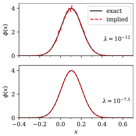
Figure 3.
Comparison of the exact (bold line) and implied (dashed line) densities for two different values of the regularization parameter . The exact density was normal with and shifted to . The top panel shows an under-regularized implied density (), while the bottom panel shows a close to optimal implied density with .
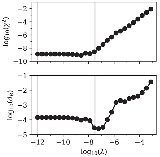
Figure 4.
Log–log plot of the squared error in prices (top panel) and the Bhattacharyya distance (bottom panel). Both measures were calculated based on a comparison between the exact input data and our implied output data for prices and densities, respectively. The input option prices were based on a Bachelier model. The related input density was a normal distribution with and shifted to . The vertical lines mark the positions of and , for which we show the implied densities in Figure 3.
For the error in prices was almost independent of . That meant that many different solutions to the optimization problem existed, which produced a basically perfect fit to the prices. This was possible since we retained a large number of singular values. In the density this manifested in the form of tiny oscillations, as can be seen in Figure 3. In other words, without regularization the input prices did not contain enough information for the optimization to yield a smooth density at the high resolution we selected for . As expected, all densities, irrespective of the value of , were non-negative.
For , the error in prices was very slightly higher, but the Bhattacharyya distance , with respect to the known normal distribution, was actually minimal, since the oscillations were suppressed.
For larger values of , the error in prices and Bhattacharyya distance increased, since the implied density was a broadened version of the original normal distribution.
The effect of regularization on the optimized parameters could also be visualized by counting the number of entries in , for which the absolute value was above a threshold a. The visualization for a few different threshold values is shown in Figure 5. Recall that the number of entries in was . Figure 5 shows that for the problem was basically unregularized, and almost all parameters had a magnitude larger than . As soon as the regularization became effective, the number of parameters with significant magnitude drastically reduced, starting with those that had the least impact on the quality of the prices.
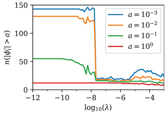
Figure 5.
Visualization of the effect of regularization on the number of relevant parameters for the implied transformed density . A larger regularization parameter led to fewer entries with significant magnitude in , i.e., regularization turned into a sparse representation of the true density . The number of entries in with a magnitude above the positive threshold a is denoted as and shown as a function of the regularization parameter . For we chose to show the axis in logarithmic scale. The figure is based on the same Bachelier model as that in Figure 3 and Figure 4. The effect of regularization is clearly visible around , where there was a sharp decrease in the number of parameters with significant magnitude.
The point where the number of parameters sharply decreased was directly related to the minimum in the Bhattacharyya distance that we observed in Figure 4. For larger values of the regularization parameter, the fit simply became worse, since relevant components of were strongly suppressed. The fit tried to compensate for this by increasing the number of other non-zero components of , but failed to achieve good accuracy.
The Bhattacharyya distance can of course only be used to select an optimal solution when the original density is known. As we see in further examples, the minimum in the Bhattacharyya distance usually corresponds to the point where the error in prices starts to increase after showing a plateau for small values of the regularization parameter .
Hence, for practical use cases, where the density is not known, we suggest calculating the solutions for multiple values of , as we did here, and selecting the solution with the highest value of that still shows close to minimal error in prices . The effect of regularization on the parameters can also be verified by an analysis, similar to what we presented in Figure 5.
3.2. Log-Normal Density
A log-normal density corresponds to the classic Black–Scholes formula for option pricing. (Black and Scholes 1973) We fixed the initial underlying price to , the volatility to , the interest rate to and the time to expiry to . We then calculated the prices of 200 Call and Put options for a uniformly discretized grid of strikes between and .
We used the so-calculated option prices to imply the density on a uniformly discretized grid with , and using our method. We retained singular values.
In summary, we recovered the log-normal distribution of the Black–Scholes model to a high degree of accuracy (see Figure 6). Further evidence is shown in Figure 7, which depicts the error in prices calculated from Equation (16) and the Bhattacharyya distance of with respect to the log-normal distribution calculated via Equation (21).
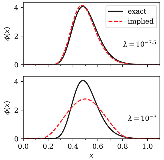
Figure 6.
Comparison of the exact (bold line) and implied (dashed line) density for two different values of the regularization parameter . The exact density was log-normal with and shifted to . The top panel shows a close to optimal regularized implied density (), while the bottom panel shows an over-regularized implied density with .
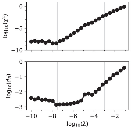
Figure 7.
Log–log plot of the squared error in prices (top panel) and the Bhattacharyya distance (bottom panel). Both measures were calculated based on a comparison between exact input data and our implied output data for prices and densities, respectively. The input option prices were based on the Black–Scholes model. The related input density was a log-normal distribution with and shifted to . The vertical lines mark the positions of and , for which we show the implied densities in Figure 6.
It is clear that the results were optimal for , where the price error and the Bhattacharyya distance were simultaneously minimized. For smaller values of the regularization parameter we observed convergence issues in the ECOS solver, probably because we retained a large number of singular values Q, which allowed for many similarly good solutions. This could probably be resolved by either fine-tuning of numerical parameters in ECOS or by reducing the number of singular values.
Figure 6 compares the exact log-normal distribution and our implied discretization for two values of the regularization parameter . The optimal solution () closely followed the log-normal distribution. Even though the less optimal solution had a slightly broader shape, it still looked similar to a log-normal distribution. Finally, we verified that all densities we implied from option prices were non-negative.
3.3. Multimodal Density
Since it has been reported that several known methods struggle with multimodal densities (Le Floc’h and Osterlee 2019a), we wanted to verify that our method also performs well in such cases. For simplicity, we considered a linear combination of normal distributions . Since the price could be calculated from an integral over the density (see Equation (1)), and since every integral was linear, we concluded that the price for an option on an underlying that was distributed according to a linear combination of normal distributions, could be calculated as the equivalent linear combination of Bachelier option prices (see Equations (23) and (24)).
We next considered a probability distribution , built from the linear combination of three normal distributions :
For the parameters, we used the values given in Table 1. If we want to be a probability distribution, we must obviously require that and that all are non-negative. Note that setting the mean value for each normal distribution implies the use of different values for the forward price in the Bachelier formulae for each term.

Table 1.
Parameters for a multimodal density. These parameters are used in Equation (25) to generate a density which is a superposition of multiple normally distributed components.
Again, we fixed the interest rate to and the time to expiry to . We then calculated the prices of 200 Call and Put options for a uniformly discretized grid of strikes between and .
We used the so-calculated option prices to imply the density on a uniformly discretized grid with , and using our method. We retained singular values.
In summary, multimodal distributions seem to pose no problem for our method. The original density is recovered with good accuracy (see Figure 8). Quantitative error estimates are shown in Figure 9, which depicts the error in prices calculated from Equation (16) and the Bhattacharyya distance of with respect to the linear combination of normal distributions calculated via Equation (21). Again, we observed that the minimum in the Bhattacharyya distance corresponded to the minimum of the price error .
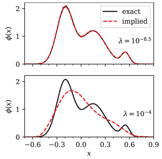
Figure 8.
Comparison of the exact (bold line) and implied (dashed line) density for two different values of the regularization parameter . The exact density is a linear combination of normal distributions, according to Equation (25), with parameters taken from Table 1. The top panel shows an optimal regularized implied density (), while the bottom panel shows an over-regularized implied density with .
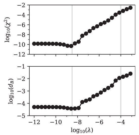
Figure 9.
Log–log plot of the squared error in prices (top panel) and the Bhattacharyya distance (bottom panel). Both measures were calculated based on a comparison between exact input data and our implied output data for prices and density, respectively. The input density was given by Equation (25), with parameters taken from Table 1. The input option prices were calculated from an equivalent linear combination of Bachelier models with the same parameters, as in Table 1. The vertical lines mark the positions of and , for which we show the implied densities in Figure 8.
In Figure 8 we show a comparison between the exact linear combination of normal distributions and our implied discretization for two values of the regularization parameter . The optimal solution () closely followed the original distribution. The solution for was a version of our initial density, in which the features were broadened to become almost indistinguishable.
3.4. Density Implied from Prices with Arbitrage
We now show that our method not only recovered known densities with high accuracy, but also carried out automatic de-arbitraging. Again, we set up a “density” as a linear combination of three normal distributions using Equation (25). However, we use quotation marks since we introduced one negative pre-factor, so that the resulting “density” contained negative “probabilities”. The parameters used in this subsection can be found in Table 2.
Table 2.
Parameters for a multimodal density. These parameters were used in Equation (25) to generate a density which was a superposition of multiple normally distributed components. This parameter set contained arbitrage, i.e., the resulting “density” contained negative “probabilities”. This was due to the negative pre-factor.
We used the Bachelier option pricing formulae (see Equations (23) and (24)) in the same way as in the multimodal case previously discussed. We set the interest rate to and the time to expiry to . We then calculated the prices of 200 Call and Put options for a uniformly discretized grid of strikes between and .
From the so-calculated option prices we implied the density on a uniformly discretized grid with , and using our method. We retained singular values.
Even prices that corresponded to partly negative “densities” could be processed using our method. In Figure 10 we show the error in prices calculated from Equation (16) and the Bhattacharyya distance. Here, special care must be taken when calculating the Bhattacharyya distance, which is not defined for partly negative “densities”. Therefore, we calculated the Bhattacharyya distance using Equation (21) with respect to the non-negative part of the input “density”, that is . However, is not truly a density. Recall that we fixed the sum of coefficients so that the integral over the density yielded unity. However, if there are negative regions, we know that the integral over the non-negative part is larger than one. Therefore, the overlap in the Bhattacharyya formula may be larger than one, so that the Bhattacharyya distance may become negative.
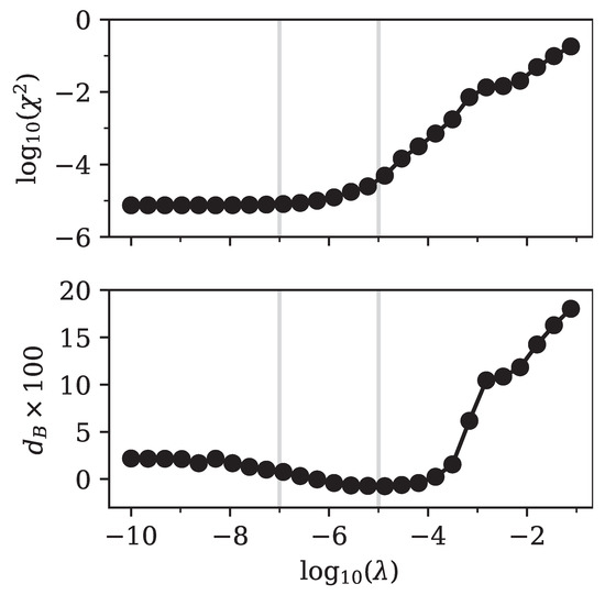
Figure 10.
Log–log plot of the squared error in prices (top panel) and log plot of the Bhattacharyya distance (bottom panel). Both measures were calculated based on a comparison between exact input data and our implied output data for prices and densities, respectively. The input density was given by Equation (25) with parameters taken from Table 2. The input option prices were calculated from an equivalent linear combination of Bachelier models with the same parameters as those in Table 2. The vertical lines mark the positions of and , for which we show the implied densities in Figure 11.
Of course, we could have normalized the non-negative part so that the integral over it was exactly one. However, we believe that such a situation may occur in practical applications and wanted to point out the consequences in detail. Therefore, we show, in Figure 10, the Bhattacharyya distance directly, instead of its logarithm.
This time, any regularization led to an increase in the pricing error . This was quite logical, since the input prices were simply not reachable with a non-negative density, both because the inputs implied negative “probabilities” and because the integral over the positive part of the input “density” was not equal to one. Hence, there is no easy rule for selecting an appropriate regularization parameter. Any regularization increases the pricing error, while it reduces the oscillations in the extracted density. Therefore, we suggest defining the necessary pricing accuracy and then selecting the largest possible regularization parameter that yields a lower pricing error.
In Figure 11 we show a comparison between the exact linear combination of normal distributions and our implied discretization for two values of the regularization parameter . Which of these extracted densities was better suited for further processing depended on the specific use case.
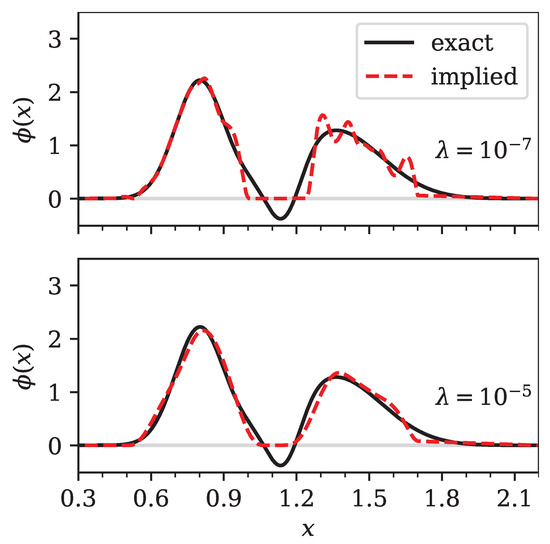
Figure 11.
Comparison of the exact (bold line) and implied (dashed line) density for two different values of the regularization parameter . The exact “density” is a linear combination of normal distributions according to Equation (25), using parameters from Table 2, which contains a region with negative probability. The top panel shows an under-regularized implied density (), while the bottom panel shows a well-regularized implied density with .
The automatic de-arbitraging feature of our method is also very useful when dealing with implied volatilities. Suppose we did not know the density from which input prices were generated. If we were to calculate implied volatilities we would usually use log-normal volatilities and simply calculate them by inverting the Black–Scholes model. This generates an implied volatility smile, which may, and in this case does, contain arbitrage. However, we could also generate an arbitrage-free volatility smile from the prices that we obtained from our optimization procedure. We calculated the implied volatilities using a simple bisection solver. We re-used the interest rate and time to expiry . However, we now also needed an initial value of the underlying, which we arbitrarily set to . Of course, in a realistic setting, this value would be known from the market.
We show the results of the log-normal implied volatility calculation in Figure 12. Clearly, the original volatility smile and our de-arbitraged version, calculated on the density with (see Figure 11, bottom panel) were very similar. The arbitrage in the original volatility smile was not directly visible. This also shows why methods that work directly with the implied volatility may introduce arbitrage, which is not immediately apparent to the user.
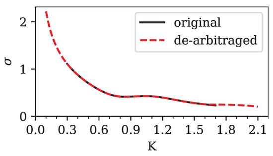
Figure 12.
Comparison of the log-normal implied volatilities (as a function of the option strike K) calculated from the input prices containing arbitrage (bold line), which were based on Equation (25) and parameters from Table 2, and the de-arbitraged prices calculated from our method (dashed line) at . The calculation of de-arbitraged implied volatilities is based on the density shown in Figure 11 (bottom panel).
Note how our method also enables us to extrapolate beyond the range of known strikes, since it gives us access to smooth non-negative density in our range of choice. The results beyond the range of strikes with known prices are certainly speculative, but consistent with the known inputs. That we obtain sensible behavior in the wings of the volatility smile without any additional effort, is another advantageous property of the sparse modeling approach.
3.5. Density Implied from S&P 500 Option Prices
It has been mentioned in the literature (Le Floc’h and Osterlee 2019a) that short-term SPX500 options pose a challenge, particularly to stochastic volatility models and the similar SVI smile model (Gatheral and Jacquier 2014), since their volatility smiles are quite steep. We imported the market data from Table 11 in Le Floc’h and Osterlee (2019a), which corresponded to SPX500 1M (one month) options on 5 February 2018. We calculated Call and Put option prices from these market data for 75 strikes in the range between 1900 and 2900, using the Black (1976) model.
We noticed that the strikes in the thousands range led to numerical problems in the ECOS solver, so we divided all strikes in the inputs by 1000. The same transformation was also applied to the forward price. This simple rescaling of the problem solved the numerical issues we encountered with the original inputs.
We used the so-calculated option prices to imply the density on a uniformly discretized grid with , and using our method. We retained singular values, which was lower than in the previous cases, because we also had fewer quoted strikes available.
The original prices were reproduced to a high degree of accuracy. In Figure 13 we show the error in prices calculated from Equation (16), which was negligible in the unregularized limit. Since the terminal density was truly unknown in this case, we could not measure the Bhattacharyya distance. As can be seen in Figure 13, any increase in the regularization parameter led to an increase in pricing error.
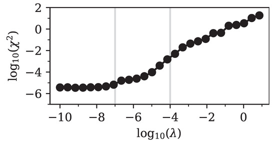
Figure 13.
Log–log plot of the squared error in prices as a function of the regularization parameter for SPX500 1M options as of 5 February 2018. The squared error was calculated from a comparison between exact input data and our implied output prices. The input option prices were calculated from the Black (1976) model with market data of Table 11 in Le Floc’h and Osterlee (2019a). The vertical lines mark the positions of and , for which we show the implied densities in Figure 14.
In Figure 14 we show the implied density for two different values of the regularization parameter . For the error in prices was still close to minimal and the density showed a pronounced spike around , followed by a very sharp decrease. For stronger regularization, such as for , the features of the density were smeared out and the error in prices increased substantially. Again, the largest possible , which still gives an error in prices close to the minimum, should be selected.
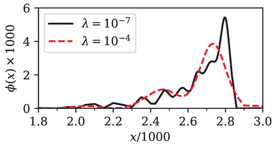
Figure 14.
Comparison of implied densities for SPX500 1M options as of 5 February 2018. A good compromise between accuracy and smoothness was achieved for (bold line), while yielded a density that contained fewer features (dashed line) and was potentially over-regularized. As explained in the main text, we rescaled both the price x of the underlying asset and the density , for numerical reasons, by a factor of 1/1000 and 1000, respectively.
Since the original data in Le Floc’h and Osterlee (2019a) is given in terms of log-normal implied volatilities, we also calculated these implied volatilities from our density at . The implied volatility was found by calculating option prices from the density using Equation (1) and then inverting the Black formula using a bisection solver for the volatility.
The comparison between input volatilities and the volatility smile extracted from our method is shown in Figure 15. The visible kink in the implied volatility around was well reproduced. Note again how our method enabled us to not only interpolate, but also extrapolate, implied volatilities even in challenging situations.
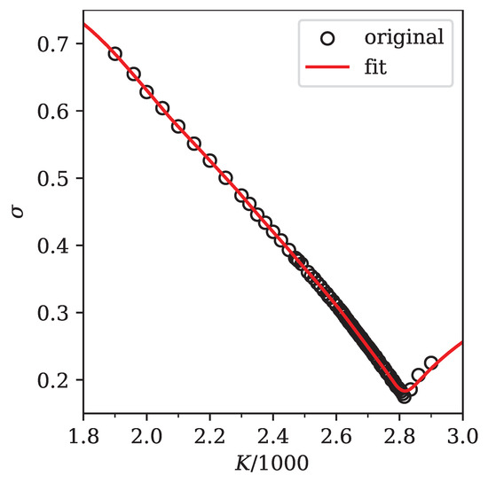
Figure 15.
Comparison of input implied volatilities (open circles) and the volatility smile provided by our method at (bold line) for SPX500 1M options as of 5 February 2018. The volatilities are shown as a function of the option strike K in units of thousands. Clearly, our method reproduced the inputs with a high degree of accuracy and, additionally, provided a sensible extrapolation of the available data.
4. Conclusions
We have presented a new method for implying terminal densities directly out of option prices. We showed that our method is able to produce arbitrage-free interpolations and extrapolations of both option prices and implied volatilities, while it does not require de-arbitraging of input prices or other pre-processing steps.
Our algorithm is based on singular value decomposition (SVD), which produces a transformation to a basis, in which the relation between prices and density is represented by a sparse model. In this sense, the number of parameters in the model Q is smaller than, or similar to, the number of input option prices M, while we may extract the density with a much larger number of discretization points N.
This property is the hallmark of any sparse model. It enables us to formulate the optimization problem for finding the density based on optimizing a small number of parameters Q. We also showed how -regularization helps in finding a density that is a good compromise between pricing error and smoothness.
Besides the trivial parameters and that define the boundaries of the interval in which the density is discretized, the only relevant parameters of our method that are visible to the user are the number of retained singular values Q, the number of input option prices M, the number of discretization points for the density N and the regularization parameter . The number of input prices M is fixed by the problem that is under investigation. We experienced good results when choosing . For N, we simply chose a large number so that we could re-calculate option prices with sufficient accuracy. For our purposes, always seemed sufficient.
In this sense, only the regularization parameter is truly up to the user’s choice. We also presented a simple rule for selecting by scanning the error in prices for a number of different values for and choosing the highest possible one with close to minimal error . In the literature, this is often referred to as the “elbow method”.
As far as we are aware, relying on optimization, and the subsequent need to choose a regularization parameter, seem to be the only drawbacks of the sparse modeling approach. Of course, our method cannot be used to directly price exotic options, while this is easily possible with stochastic volatility models once they have been calibrated. That, however, is not the topic of the present investigation.
Barring these restrictions, the advantages of our method are clear. The mathematics behind our method is simple and easy to understand. Using the numerical libraries mentioned, the algorithm is also easy to implement. Our own implementation in the Python programming language consists of fewer than 100 lines of code. The accuracy of our method proved to be excellent for all artificial and realistic examples we investigated.
Furthermore, our algorithm is robust against defects in the input data, such as arbitrage. Since it works directly with the terminal density, our method can also be used to extrapolate option prices and implied volatilities in an arbitrage-free manner far beyond the available range of market quotes. Having sensible behavior in the wings of the volatility smile, without any further effort, is quite rare an occurrence and is certainly a strong advantage of our method.
What makes our method stand out from other available approaches, is that choosing a polynomial or other basis for the regression is not necessary, because a suitable orthogonal basis is automatically constructed by the SVD. In this sense, our method is truly model-free.
At present, our algorithm works with options of multiple strikes, but with a single time to maturity. In future works, we would like to investigate extensions to multiple maturities, such that the whole volatility surface can be calibrated consistently.
Such an extension would enable us to use our method to calibrate a local volatility (Derman and Kani 1994; Dupire 1994) or local stochastic volatility model (Lipton 2002; Lipton et al. 2014), which we could then use to price options with American exercise (Andersen and Lake 2021; Andersen et al. 2016; Healy 2021), barrier options (Clark 2010; Guterding and Boenkost 2018) or other exotic products. Since our method is robust against defects in the market data, such an extension should be particularly helpful in situations where the market data are potentially stale or only a few strikes are quoted. For example, this could be the case in markets for cryptocurrency (Hou at al. 2020; Yang and Hamori 2021a; Zulfiqar and Gulzar 2021), energy (Benth et al. 2008; Fabbiani et al. 2020; Yang 2021b) or foreign exchange options (Clark 2010; Guterding and Boenkost 2018), and also for Equity options (Healy 2021) with less popular underlyings.
Funding
This research was funded by Technische Hochschule Brandenburg, University of Applied Sciences.
Data Availability Statement
No new data were created or analyzed in this study. Data sharing is not applicable to this article.
Conflicts of Interest
The authors declare no conflict of interest.
Abbreviations
The following abbreviations are used in this manuscript:
| SVD | Singular Value Decomposition |
| LV | Local Volatility |
| LSV | Local Stochastic Volatility |
| SABR | Stochastic Alpha, Beta, Rho |
| SPX500 | Standard & Poor’s 500 Stock Index |
| ITM | In-The-Money |
| OTM | Out-Of-The-Money |
Appendix A. Treatment of In-the-Money Options in the Error Function Calculation
When considering Call and Put options with arbitrary strike, the prices of the options may differ by several orders of magnitude if some options are in-the-money. In-the-money options are executed with large probability and, hence, have a high price.
However, if the prices in our problem differ by orders of magnitude, the calculated error function is dominated by the options with the largest price, which are, unfortunately, those that depend only on the tail of the probability distribution . This is not desirable, since we are usually equally interested in all regions of the density, or even more so in the density close to at-the-money. This problem can be solved by transforming prices of in-the-money options to prices of out-of-the-money options.
Let F define the forward price of the underlying asset at time T. Then a Call option with strike K is considered in-the-money if . A Put option is considered in-the-money if . Conversely, a Call option is out-of-the-money if and a Put option is out-of-the-money if .
Let denote the price of a European Call option with strike K and expiry at T and let denote the price of a Put option with the same strike and expiry. If is the value of the underlying asset at , then, for European options with the same strike and the same time to expiry , Put–Call-parity holds:
So, for all in-the-money Call options, we may calculate the price of the respective out-of-the-money Put option from Equation (A1). Likewise, for all in-the-money Put options, we may calculate the price of the respective out-of-the-money Call option from Equation (A1).
In this way, we can easily restrict the prices in our optimization problem to out-of-the-money and at-the-money options, which all have prices with roughly the same order of magnitude. Hence, the error function is not dominated by the options that depend only on the tails of the probability distribution.
Although we did not have to apply this transformation from ITM to OTM options in the present manuscript, we believe it makes sense to document this idea, in case our readers encounter problems with ITM options when applying our method.
Appendix B. Ideas for Performance Optimization
The main tunable parameters that influence the performance of the algorithm we presented are the number of retained singular values Q and the number of discretization points for the density N. Since Q is also the number of parameters in the optimization problem, it is clear that reducing Q could lead to faster convergence of the optimization algorithm. Figure 5 clearly shows that after regularization only a few relevant parameters remained. Therefore, the remaining parameters with negligible weight could also be removed, before we even started the optimization process, by choosing a lower value of Q.
Based on our analysis of singular values in Figure 2 we could expect that a reduction of Q would first result in discarding of the less relevant parameters and would then progress to removing more relevant ones if Q further reduced. However, the manner by which this depends on input prices is not clear. Therefore, this issue needs more analysis before we can give any definitive conclusion, but this was not the main point of the present manuscript.
The second opportunity for speeding up the algorithm is to reduce the number of discretization points for the density N. The point of having more discretization points than input strikes is to have a high enough resolution to be able to recalculate the input option prices with sufficient accuracy, so as to enable use of the implied density for interpolation. Since N determines the effort for the partial SVD, the basis transformations and the checking of the constraints in the optimization problem, it is worth thinking about a reduction of N. We suggest first checking whether a reduction in N increases the error in prices . If the density is required for an interpolation of prices or implied volatilities, first interpolating the density linearly and then calculating prices and implying volatilities, based on the interpolated densities, is always an option. Since a linear interpolation of a non-negative function is also non-negative, we can be sure that this procedure would not introduce negative densities, i.e., arbitrage. Linear interpolation of the density also does not violate the constraint that the trapezoidal integral over the density must be equal to unity.
If our method is used in a live environment, where the density is implied on every market data update, or on every couple of market data updates, it may be useful to warm-start the numerical solver from the previous solution to accelerate convergence.
Note
| 1 | https://github.com/danielguterding/svdensity (accessed on 21 April 2023). |
References
- Agrawal, Akshay, Robin Verschueren, Steven Diamond, and Stephen Boyd. 2018. A rewriting system for convex optimization problems. Journal of Control and Decision 5: 42. [Google Scholar] [CrossRef]
- Aït-Sahalia, Yacine, Peter J. Bickel, and Thomas M. Stoker. 2001. Goodness-of-fit tests for kernel regression with an application to option implied volatilities. Journal of Economics 105: 363. [Google Scholar] [CrossRef]
- Andersen, Leif, and Mark Lake. 2021. Fast American Option Pricing: The Double-Boundary Case. Wilmott 2021: 30. [Google Scholar] [CrossRef]
- Andersen, Leif, Mark Lake, and Dmitri Offengenden. 2016. High-performance American option pricing. Journal of Computational Finance 20: 39. [Google Scholar] [CrossRef]
- Andreasen, Jesper, and Brian Norsk Huge. 2011. Volatility Interpolation. Risk 24: 76. [Google Scholar] [CrossRef]
- Bachelier, Louis. 1901. Théorie mathématique du jeu. Annales Scientifiques de l’Ecole Normale Supérieure 18: 143. [Google Scholar] [CrossRef]
- Baker, Glyn, Reimer Beneder, and Alex Zilber. 2004. FX Barriers with Smile Dynamics. Available online: https://ssrn.com/abstract=964627 (accessed on 21 April 2023).
- Benth, Fred Espen, Jūratė Šaltytė Benth, and Steen Koekebakker. 2008. Stochastic Modeling of Electricity and Related Markets. Singapore: World Scientific. ISBN 978–9-812-81230-8. [Google Scholar]
- Bhattacharyya, Anil. 1943. On a measure of divergence between two statistical populations defined by their probability distributions. Bulletin of the Calcutta Mathematical Society 35: 99. [Google Scholar]
- Black, Fischer. 1976. The pricing of commodity contracts. Journal of Financial Economics 3: 167. [Google Scholar] [CrossRef]
- Black, Fischer, and Myron Scholes. 1973. The Pricing of Options and Corporate Liabilities. Journal of Political Economy 81: 637. [Google Scholar] [CrossRef]
- Boyd, Stephen, Neal Parikh, Eric Chu, Borja Peleato, and Jonathan Eckstein. 2010. Distributed Optimization and Statistical Learning via the Alternating Direction Method of Multipliers. Foundations and Trends® in Machine Learning 3: 1. [Google Scholar] [CrossRef]
- Breeden, Douglas T., and Robert H. Litzenberger. 1978. Prices of State-Contingent Claims Implicit in Option Prices. Journal of Business 51: 621. [Google Scholar] [CrossRef]
- Carr, Peter, and Roger Lee. 2009. Volatility Derivatives. Annual Review of Financial Economics 1: 319. [Google Scholar] [CrossRef]
- Carr, Peter, Andrey Itkin, and Dmitry Muravey. 2022. Semi-analytical pricing of barrier options in the time-dependent Heston model. arXiv. [Google Scholar] [CrossRef]
- Choi, Jaehyuk, Minsuk Kwak, Chyng Wen Tee, and Yumeng Wang. 2022. A Black-Scholes user’s guide to the Bachelier model. Journal of Futures Markets 42: 959. [Google Scholar] [CrossRef]
- Clark, Iain. 2010. Foreign Exchange Option Pricing: A Practitioners Guide. Chichester: John Wiley & Sons. ISBN 978-0-470-68368-2. [Google Scholar]
- Derman, Emanuel, and Iraj Kani. 1994. Riding on a smile. Risk 7: 32. [Google Scholar]
- Derman, Emanuel, and Michael. B. Miller. 2016. The Volatility Smile. Hoboken: John Wiley & Sons. ISBN 978-1-118-95916-9. [Google Scholar]
- Diamond, Steven, and Stephen Boyd. 2016. CVXPY: A Python-embedded modeling language for convex optimization. Journal of Machine Learning Research 17: 2909. [Google Scholar]
- Domahidi, Alexander, Eric Chu, and Stephen Boyd. 2013. ECOS: An SOCP Solver for Embedded Systems. Paper presented at European Control Conference, Zurich, Switzerland, July 17–19; pp. 3071–3076. [Google Scholar]
- Dupire, Bruno. 1994. Pricing with a smile. Risk 7: 18. [Google Scholar]
- Egloff, Daniel, Markus Leippold, and Liuren Wu. 2010. The Term Structure of Variance Swap Rates and Optimal Variance Swap Investments. Journal of Financial and Quantitative Analysis 45: 1279. [Google Scholar] [CrossRef]
- Fabbiani, Emanuele, Andrea Marziali, and Giuseppe De Nicolao. 2020. Vanilla-option-pricing: Pricing and market calibration for options on energy commodities. Software Impacts 6: 100043. [Google Scholar] [CrossRef]
- Gatheral, Jim. 2006. The Volatility Surface: A Practitioner’s Guide. Hoboken: Wiley Finance. ISBN 978-0-471-79251-2. [Google Scholar]
- Gatheral, Jim, and Antoine Jacquier. 2014. Arbitrage-free SVI volatility surfaces. Quantitative Finance 14: 59. [Google Scholar] [CrossRef]
- Guterding, Daniel. 2021. Inventory effects on the price dynamics of VSTOXX futures quantified via machine learning. Journal of Finance and Data Science 7: 126. [Google Scholar] [CrossRef]
- Guterding, Daniel, and Wolfram Boenkost. 2018. The Heston stochastic volatility model with piecewise constant parameters—Efficient calibration and pricing of window barrier options. Journal of Computational and Applied Mathematics 343: 353. [Google Scholar] [CrossRef]
- Hagan, Patrick, Andrew Lesniewski, and Diana Woodward. 2015. Probability Distribution in the SABR Model of Stochastic Volatility. In Large Deviations and Asymptotic Methods in Finance. Edited by Peter K. Friz, Jim Gatheral, Archil Gulisashvili, Antoine Jacquier and Josef Teichmann. Cham: Springer Proceedings in Mathematics & Statistics, vol. 110. [Google Scholar]
- Hagan, Patrick, Deep Kumar, and Andrew Lesniewski. 2001. Managing Smile Risk. Wilmott 1: 84. [Google Scholar]
- Healy, Jherek. 2021. Applied Quantitative Finance for Equity Derivatives. Lulu.com: ISBN 978-1-716-19039-1. [Google Scholar]
- Heston, Steven L. 1993. A Closed-Form Solution for Options with Stochastic Volatility with Applications to Bond and Currency Options. The Review of Financial Studies 6: 327. [Google Scholar] [CrossRef]
- Hou, Ai Jun, Weining Wang, Cathy Y. H. Chen, and Wolfgang Karl Härdle. 2020. Pricing Cryptocurrency Options. Journal of Financial Econometrics 18: 250. [Google Scholar]
- Jäckel, Peter. 2014. Clamping down on arbitrage. Wilmott 2014: 54. [Google Scholar] [CrossRef]
- Jiang, Yixiao. 2020. A Hausman Test for Partially Linear Models with an Application to Implied Volatility Surface. Journal of Risk and Financial Management 13: 287. [Google Scholar] [CrossRef]
- Kahalé, Nabil. 2004. An arbitrage-free interpolation of volatilities. Risk 17: 102. [Google Scholar]
- Le Floc’h, Fabien, and Cornelis W. Osterlee. 2019a. Model-free stochastic collocation for an arbitrage-free implied volatility: Part I. Decisions in Economics and Finance 42: 679. [Google Scholar] [CrossRef]
- Le Floc’h, Fabien, and Cornelis W. Osterlee. 2019b. Model-free stochastic collocation for an arbitrage-free implied volatility: Part II. Risks 7: 30. [Google Scholar] [CrossRef]
- Lipton, Alexander. 2002. The vol smile problem. Risk 15: 61. [Google Scholar]
- Lipton, Alexander, Andrey Gal, and Andris Lasis. 2014. Pricing of vanilla and first-generation exotic options in the local stochastic volatility framework: Survey and new results. Quantitative Finance 14: 1899. [Google Scholar] [CrossRef]
- Lorig, Matthew, Stefano Pagliarani, and Andrea Pascucci. 2017. Explicit Implied Volatilities for Multifactor Local-Stochastic Volatility Models. Mathematical Finance 27: 926. [Google Scholar] [CrossRef]
- Mixon, Scott. 2002. Factors explaining movements in the implied volatility surface. Journal of Futures Markets 22: 915. [Google Scholar] [CrossRef]
- O’Donoghue, Brendan, Eric Chu, Neal Parikh, and Stephen Boyd. 2016. Conic Optimization via Operator Splitting and Homogeneous Self-Dual Embedding. Journal of Optimization Theory and Applications 169: 1042. [Google Scholar] [CrossRef]
- Otsuki, Junya, Masayuki Ohzeki, Hiroshi Shinaoka, and Kazuyoshi Yoshimi. 2020. Sparse Modeling in Quantum Many-Body Problems. Journal of the Physical Society of Japan 89: 012001. [Google Scholar] [CrossRef]
- Tian, Yu, Zili Zhu, Geoffrey Lee, Thomas Lo, Fima Klebaner, and Kais Hamza. 2014. Pricing Window Barrier Options with a Hybrid Stochastic-Local Volatility Model. Paper presented at 2014 IEEE Conference on Computational Intelligence for Financial Engineering & Economics (CIFEr), London, UK, March 27–28. [Google Scholar]
- Xing, Yuhang, Xiaoyan Zhang, and Rui Zhao. 2010. What Does the Individual Option Volatility Smirk Tell Us About Future Equity Returns? Journal of Financial and Quantitative Analysis 45: 641. [Google Scholar] [CrossRef]
- Yang, Lu. 2021. Idiosyncratic information spillover and connectedness network between the electricity and carbon markets in Europe. Journal of Commodity Markets 25: 100185. [Google Scholar] [CrossRef]
- Yang, Lu, and Shigeyuki Hamori. 2021. The role of the carbon market in relation to the cryptocurrency market: Only diversification or more? International Review of Financial Analysis 77: 101864. [Google Scholar] [CrossRef]
- Zhu, Song-Ping, and Guang-Hua Lian. 2012. An analytical formula for VIX futures and its applications. Journal of Futures Markets 32: 166. [Google Scholar] [CrossRef]
- Zulfiqar, Noshaba, and Saqib Gulzar. 2021. Implied volatility estimation of bitcoin options and the stylized facts of option pricing. Financial Innovation 7: 67. [Google Scholar] [CrossRef] [PubMed]
Disclaimer/Publisher’s Note: The statements, opinions and data contained in all publications are solely those of the individual author(s) and contributor(s) and not of MDPI and/or the editor(s). MDPI and/or the editor(s) disclaim responsibility for any injury to people or property resulting from any ideas, methods, instructions or products referred to in the content. |
© 2023 by the author. Licensee MDPI, Basel, Switzerland. This article is an open access article distributed under the terms and conditions of the Creative Commons Attribution (CC BY) license (https://creativecommons.org/licenses/by/4.0/).