Article

Backward Deep BSDE Methods and Applications to Nonlinear Problems

Corporate Model Risk, Wells Fargo, New York, NY 10017, USA
*
Author to whom correspondence should be addressed.
Risks 2023, 11(3), 61; https://doi.org/10.3390/risks11030061
Submission received: 2 November 2022 / Revised: 24 February 2023 / Accepted: 10 March 2023 / Published: 16 March 2023

Abstract

:
We present a pathwise deep Backward Stochastic Differential Equation (BSDE) method for Forward Backward Stochastic Differential Equations with terminal conditions that time-steps the BSDE backwards and apply it to the differential rates problem as a prototypical nonlinear problem of independent financial interest. The nonlinear equation for the backward time-step is solved exactly or by a Taylor-based approximation. This is the first application of such a pathwise backward time-stepping deep BSDE approach for problems with nonlinear generators. We extend the method to the case when the initial value of the forward components X can be a parameter rather than fixed and similarly to also learn values at intermediate times. We present numerical results for a call combination and for a straddle, the latter comparing well to those obtained by Forsyth and Labahn with a specialized PDE solver.

1. Introduction

As proposed in Han and Jentzen (2017), deep learning (DL) and deep neural networks (DNN) can be used to solve high-dimensional nonlinear PDEs by converting them to Forward Backward Stochastic Differential Equations (FBSDE) and building neural networks to learn the control and initial value of the corresponding stochastic control problem. They use their method on, for instance, a differential rates problem, as studied in Mercurio (2015), for a combination of two call options. Hientzsch (2021) also gives an overview of pricing different instruments in quantitative finance via deep BSDE and FBSDE.
To summarize, deep BSDE methods rewrite the FBSDE problem into a stochastic control problem where one searches for a control (ultimately approximating the gradient of the solution) and an initial value or initial value function which minimize certain loss functions. The minimization typically occurs through stochastic gradient descent approaches and variants (such as Adam), where the stochastic gradient with respect to the parameters of the control and of the initial value function is obtained from a mini-batch of realizations of the underlying dynamics (X) and corresponding realizations of the solution of the BSDE (Y) given the current control Π . The forward deep BSDE methods (first described in Han et al. (2018)) and the backward deep BSDE methods described here differ by how the realization of Y is computed given the current control and the realization of X and also by the loss function to be minimized. These pathwise deep BSDE methods have the advantage that one only needs to implement a discretization of the forward dynamics X and a pathwise computation of the backward dynamics for Y and the loss function generically in a deep learning framework such as TensorFlow and can use standard deep learning techniques. They also can be implemented for very high-dimensional problems avoiding or at least mitigating the curse of dimensionality.
Han et al. (2018) propose time-stepping both forward and backward SDE forward in time and transform the final value problem to a stochastic control problem in which the objective function measures how well the given final value has been approximated. We call their method the ”forward deep BSDE” method since it time-steps the BSDE forward. Wang et al. (2018) consider a BSDE with zero drift term which can be trivially time-stepped backwards and propose and demonstrate forward and backward methods with fixed X 0 , describing the first pathwise backward deep BSDE method. Liang et al. (2021) solve BSDEs with linear generators with both forward and backward methods. They indicate a Taylor expansion approach for nonlinear generators, without giving details or results for nonlinear problems. We describe the general approach and the application to the differential rates setting for two variants of this pathwise backward deep BSDE method, which is, to the best of our knowledge, the first application of this pathwise backward method to nonlinear problems.
The backward method starts with the given final value at maturity and then time-steps the BSDE backwards until a given initial time t 0 , which is assumed to be 0 without loss of generality in this paper. In continuous time and complete markets, a trading strategy can completely eliminate randomness; thus, all realizations of Y t 0 (initial value of derivative) for the same initial risk factors X t 0 should have the same value. Thus, if we minimize a measure of the range of Y t 0 , we should obtain a minimum of 0 and a risk-eliminating trading strategy. In the time-discrete and/or incomplete setting, the randomness can no longer be eliminated, but its impact can be minimized. In the pathwise backward methods, the variance of Y t 0 serves as that measure—either with respect to a Monte Carlo mean or a to-be-learned parameter. Similarly, for random X t 0 , we minimize the square distance from an also to-be-determined function Yinit ( X t 0 ) represented by a DNN. This extension to random X t 0 is new.
We consider the differential rates problem together with Black–Scholes dynamics for European options. To force nonlinear behavior, one can consider, for example, a linear combination of calls with coefficients with opposite signs or a straddle. Differential rates mean that positive cash balances in the trading strategy accrue interest at a lower lending rate, while negative cash balances (debts/loans) accrue interest at a higher borrowing rate.
For the differential rates problem, (Han and Jentzen 2017, Section 4.4) mention a nonlinear PDE which can be solved by appropriate nonlinear PDE solvers in small dimensions (see, for instance, Forsyth and Labahn (2007)). For a more general setting, Mercurio (2015) presents PDEs and proposes PDE solution or binomial tree methods. None of these methods work in higher dimensions due to the curse of dimensionality. All these methods require problem-specific implementations of nonlinear PDE or tree solvers.
There are other approaches to such nonlinear problems, including in high dimensions, that also rely on the equivalent FBSDE formulation. As mentioned above, Han and Jentzen (2017) solve a nonlinear differential rates problem with their pathwise forward deep BSDE method. Huré et al. (2020) solves nonlinear problems by a BSDE rollback method, where the solution and its gradient at each time-step are sequentially learned by minimizing the residual of the time-discretized BSDE. Warin (2018) solve nonlinear problems by repeatedly nested Monte Carlo. While somewhat straightforward to implement, this only works for shorter maturities and requires substantial computational resources. Raissi (2018) solves the BSDE by adding loss terms for the residuals of all time-steps to the usual final loss term. Training for such complex loss functions can be quite challenging and unreliable and might not lead to solutions that satisfy all constraints and loss functions equally well, and standard stochastic optimization methods often struggle to optimize well. None of these works except Han and Jentzen (2017) solve the differential rates problem.
In this paper, we first introduce FBSDE for general nonlinear problems, with particular details for the differential rates problem, time-discretize them, and then derive exact solutions and Taylor approximations for the backward step problem. We then quickly describe the forward and backward deep BSDE approaches that we consider—both the batch-variance variant already described in the literature but also the novel initial variable and network versions, the last one for varying or random X t 0 , together with a computational graph for the network version. Then, we apply these methods to the differential rates problem for the call combination case from (Han and Jentzen 2017, Section 4.4) and for the straddle case from Forsyth and Labahn (2007). We compare the results for a case with fixed X t 0 and for a case with varying X t 0 with the results from Forsyth and Labahn (2007) and see that they agree well. Finally, we conclude.

2. FBSDE for Nonlinear Problems

We are interested in solving a nonlinear PDE for a single function u that depends on time t and an n-dimensional state vector x of the following general form:
u t t , x + L t u t , x + f t , x , u t , x , x u t , x = 0 ,
with
L t u t , x : = 1 2 Tr ( σ σ T ) t , x Hess x u t , x + μ t , x x u t , x ,
where x u is the gradient vector with respect to the x and Hess x u is the Hessian matrix with respect to the x, with μ t , x R n and σ t , x R n , n being appropriate vector and matrix functions of their arguments, together with terminal condition at maturity T given as
u ( T , x ) = g ( x ) .
A nonlinear Feyman–Kac theorem1 shows that the solution of the above PDE also satisfies the following FBSDE system under appropriate assumptions:
The forward SDE (FSDE) for the vector X t R n :
d X t = μ t , X t d t + σ t , X t d W t ,
and the backward SDE (BSDE) in terms of strategy Π t R n :
d Y t = f t , X t , Y t , Π t d t Π t T σ t , X t d W t ,
with terminal condition2
Y T = g ( X T ) ,
where
Y t = u ( t , X t ) , Π t = X u ( t , X t ) .
In terms of pricing applications in finance, X t is the vector of values of the underlying assets, and g ( X T ) is the final payoff of the European option that one tries to replicate with a self-financing portfolio in the underlying asset(s) and a remaining cash position. That portfolio will contain π j ( t ) worth of the jth underlying asset (corresponding to index j in the vector X t ), and Π t is the vector of the π j ( t ) . The portfolio (including cash position) is worth Y t at time t.
Now, Y t or equivalently u ( t , X t ) represent the needed wealth at t to exactly or approximately replicate the payoff when starting at X t at time t. One can thus define price (by replication) price ( t , X t ; X T g ( X T ) ) as the solution of the FBSDE and/or the nonlinear PDE. In linear pricing, one has
price ( t , X t ; X T g ( X T ) ) = price ( t , X t ; X T g ( X T ) ) .
In nonlinear pricing, these two prices are no longer necessarily the same but will give an upper and a lower price.
Using the Euler–Maruyama method to discretize time direction forward for both X t and Y t , we have
X t i + 1 = X t i + μ ( t i , X t i ) Δ t i + σ ( t i , X t i ) Δ W i
and
Y t i + 1 = Y t i f t i , X t i , Y t i , Π t i Δ t i + Π t i T σ ( t i , X t i ) Δ W i .

2.1. Backward Time-Stepping

As discussed in the introduction, in deep BSDE methods, we compute pathwise realizations of Y given pathwise realizations of X. Since the FBSDE that we are considering are decoupled, a realization of X can be computed independently and ahead of the realization of Y. In the pathwise backward deep BSDE methods, we compute the realization of Y backwards, starting from a given final value Y T = g ( X T ) and using the realizations of Δ W i from X. In terms of filtration, this means that we are operating under a filtration that has all the information about W t until t = T and are measurable with respect to information about X and W up to time T (and not time t as in the forward method). Since we are using realizations of X and corresponding realizations of Y given the current strategy Π · to compute gradients with respect to strategy parameters, the strategy can be assumed known. Thus, the formulas in this subsection all contain realizations, not random variables.

2.1.1. Exact Backward Time-Stepping

To backward step in time direction, we rewrite (10) as
Y t i f t i , X t i , Y t i , Π t i Δ t i = Y t i + 1 Π t i T σ ( t i , X t i ) Δ W i
and solve for Y t i .
For a differential rates setup in a risk-neutral measure, the f generator function in the BSDE is
f ( t , X t , Y t , Π t ) = r l ( t ) Y t + ( r b ( t ) r l ( t ) ) j = 1 n π j ( t ) Y t + .
This driver expresses that all assets X j ( t ) and positive cash balances grow at a risk-neutral rate r l ( t ) unless the cash position Y t j = 1 n π j ( t ) is negative, and that negative cash balance will grow at a rate r b ( t ) corresponding to the higher borrowing rate as compared with the lower or equal lending rate.
There are two cases for Equation (12):
(1). If j = 1 n π j ( t ) > Y ( t ) :
f ( t , X t , Y t , Π t ) = r l ( t ) Y t + ( r b ( t ) r l ( t ) ) j = 1 n π j ( t ) Y t .
Inserting this into Equation (11) and solving, we obtain
Y t i = Y t i + 1 + r b ( t i ) r l ( t i ) j = 1 n π j ( t i ) Δ t i Π t i T σ ( t i , X t i ) Δ W i 1 + r b ( t i ) Δ t i .
(2). If j = 1 n π j ( t ) Y ( t ) :
f ( t , X t , Y t , Π t ) = r l ( t ) Y t .
Inserting this into Equation (11) and solving, we obtain
Y t i = Y t i + 1 Π t i T σ ( t i , X t i ) Δ W i 1 + r l ( t i ) Δ t i .
However, we do not know Y t i before solving the nonlinear Equation (11) for it. From (14) and (16) and the conditions involving Y t i , we obtain that the condition Y t i < j = 1 n π j ( t i ) is equivalent to
Y t i + 1 < 1 + r l ( t i ) ) Δ t i j = 1 n π j ( t i ) + Π t i T σ ( t i , X t i ) Δ W i
and the same for the relation with ≥. Thus, if (17) is satisfied, we use (14), otherwise (16).

2.1.2. Time-Stepping from Taylor Expansion

By a first-order Taylor expansion, we have
f t i , X t i , Y t i , Π t i T σ ( t i , X t i ) f t i , X t i , Y t i + 1 , Π t i T σ ( t i , X t i ) f Y t i , X t i , Y t i + 1 , Π t i T σ ( t i , X t i ) Y t i + 1 Y t i .
Inserting this into Equation (11) and solving for Y t i , we have the following:
Y t i = Y t i + 1 + f t i , X t i , Y t i + 1 , Π t i T σ ( t i , X t i ) Δ t i Π t i T σ ( t i , X t i ) Δ W i 1 f Y t i , X t i , Y t i + 1 , Π t i T σ ( t i , X t i ) Δ t .
Note that f and f u are evaluated at Y t i + 1 .
With the same setup for the differential rates problem, it is clear that there are only two possible forms for f:
(1). If j = 1 n π j ( t i ) > Y t i + 1 :
f ( t i , X t i , Y t i + 1 , Π t i ) = r l ( t i ) Y ( t i ) + ( r b ( t i ) r l ( t i ) ) j = 1 n π j ( t i ) Y t i + 1
and
f Y = r b ( t i ) .
Inserting this into Equation (19), we obtain the same (14).
(2). If j = 1 n π j ( t i ) Y t i + 1 :
f ( t i , X t i , Y t i + 1 , Π t i ) = r l ( t i ) Y t i + 1
and
f Y = r l ( t i ) .
Inserting this into Equation (19), we again obtain (16).
Notice that both the exact and Taylor backward steps have the same form (14) and (16); the difference is in the conditions when they are applied.

3. Deep BSDE Approach

3.1. Forward Approach

As introduced in Han and Jentzen (2017), with forward time-stepped Equations (9) and (10), one minimizes the loss function
E ( | | Y T F , Π g ( X N ) | | 2 )
over parameters of the strategies Π · and over initial value Y 0 , where Y T F , Π is the result of forward stepping (10) with strategy vector Π .
The initial portfolio value Y 0 is a parameter of the minimization problem, as are all the parameters of the DNN functions π i ( t i , X t i ) treated as functions of X t i (that give the stochastic vector process Π t as value of the holdings of the risky underlying securities in the portfolio). Since X 0 is fixed, instead of learning a function π 0 ( X 0 ) , one learns a parameter π 0 . Alternatively, one can learn a single function π ( t i , X t i ) as function of t i and X t i , which means that all the parts of the computational graph that represent the evaluation of π ( t , x ) share the same DNN parameters.3 The minimization problem is then solved with standard deep learning approaches. For the case of random X 0 , one also learns the initial value of Y 0 as a function Yinit ( X 0 ) of X 0 using the same loss function.
The minimization is typically implemented through mini-batch stochastic gradient descent and similar approaches, such as Adam. The gradients of the expected value with respect to the trainable parameters are approximated by the gradients of the empirical sum over the loss function as evaluated on a number of trajectories. In this work, we generate new trajectories for each mini-batch for each epoch/stochastic gradient descent step, and we tested both on fixed testing batches as well as freshly generated batches. In general, strategies and initial value functions will be somewhat noisy, since the approximation of the expectation respective its gradient will depend on the mini-batch size. Such noise can be reduced by increasing the mini-batch size or by various kinds of postprocessing. Given a strategy Π and keeping it fixed, one can also compute a refined Yinit ( X 0 ) by performing a separate optimization only on the parameters of Yinit .

3.2. Backward Approach

In the backward approach, one time-steps Equation (9) forward but time-steps Equation (10) backward, starting from Y T = g ( X T ) . As discussed in the previous section, one can use an analytical solution of (11) or some Taylor expansion approach. Using either approach, one will obtain an expression or implementation
Y t i = ybackstep ( t i , Y t i + 1 , X t i , Π t i , Δ W i ) .
For the differential rates setup, the backward step ybackstep is given by (14) and (16) depending on whether Y t i + 1 satisfies (17) or not (for the exact step), or whether j = 1 n π j ( t i ) Y t i + 1 or not (for the Taylor step). In general, ybackstep can be any exact or approximate solution of (11).
As discussed before, the time-stepping of both (9) (forward) and (10) (backward) occurs in a single realization—one generates a realization Δ W i for all i, simulates X t i for all i from (9) and then performs the time-stepping for this specific realization for Y . A little bit more formally, let us define recursively backwards for any given current strategy function π ( t , x ) the following random variables Y π that are measurable as of time T: Y T π = Y t N π = g ( X T ) and
Y t i π ( ω ) = ybackstep ( t i , Y t i + 1 π ( ω ) , X t i ( ω ) , π ( t i , X t i ( ω ) ) , Δ W i ( ω ) )
realization by realization. This is a well-defined sequence of random variables, all measurable as of T.
For fixed X 0 , the loss function used in Wang et al. (2018) and Liang et al. (2021) is
var ( Y 0 π )
and one optimizes over functions π to find the strategy that minimizes this initial variance. (In the limit for vanishing time-steps, the gradient of the PDE solution will lead to zero variance).
For the stochastic gradient descent approaches, this variance will be approximated by the variance over the current mini-batch. Thus, for the mini-batch stochastic gradient step, the loss function will be the mini-batch variance
E ( | | Y 0 π Y ¯ 0 | | 2 ) ,
where Y ¯ 0 will be the mean over the mini-batch. Similarly to before, approximating the expectation with a finite sum over the mini-batch will introduce noise into the optimization and into the computation of Y ¯ 0 , which depends on the size of the mini-batch.
Thus, for estimates of the initial value of the instrument, one does not necessarily have to use only the last mini-batch mean, one can compute the mean of Y 0 π over a larger sample of paths or batches generated with a fixing trading strategy. Instead of using the mini-batch mean in the loss function, one can learn Y ¯ 0 as a parameter/variable (resulting in the same loss function but with different meaning of Y ¯ 0 = Yinit ).
Once X 0 is random, one can no longer use batch variance in a straightforward way. Instead (and inspired by the parameter version just discussed), one uses a loss function
E ( | | Y 0 π Yinit ( X 0 ) | | 2 ) ,
where the Yinit ( X 0 ) is a function represented by a DNN which is learned as part of the DL approaches.
Restating more formally again, we can define
Y 0 π = Yinit ( X 0 ; π ) = E [ Y 0 π | X 0 ]
and define a loss function4
L ( π ) = E ( | | Y 0 π Yinit ( X 0 ; π ) | | 2 ) .
We now are solving a (time-discrete but continuous in space) stochastic control problem
π * = argmin π L ( π )
and we define u 0 * ( X 0 ) = Yinit ( X 0 ; π * ) . We expect that π * will be an approximation (up to time-discretization error) for the gradient of the solution of the FBSDE (and thus PDE) in t = 0 T and u 0 * will be an approximation of the solution at time t = 0 . Proceeding similarly for arbitrary t, we can similarly obtain approximations of the solution at any time t in 0 T .
We solve (32) by gradient-based optimization methods to iteratively improve strategies until we obtain a minimum. The involved expectations cannot be analytically computed as functions of π , so one needs to approximate them by sampling. As discussed above, one uses mini-batch stochastic gradient descent and methods based on such (such as Adam). Moreover, instead of exactly determining the Yinit function as a conditional expectation given a strategy π , we update parameters for both π and Yinit at the same time.
As an illustration, the computational graph to compute a single sample for the empirical loss function for the backward method with random X 0 is shown in Figure 1. (For the initial variable version for fixed X 0 , both Y i n i t and Π 0 would be variables independent of X 0 , rather than networks depending on X 0 , and X 0 would be an input.) First, one simulates X forward, starting at the first time-step, proceeding through intermediate time-steps, and reaching the final time-step, according to (9). At the final time-step, Y T ( ω ) is set to g ( X T ) , and backward steps ybstep are taken (as discussed in Section 2.1), proceeding throughintermediate steps, until one reaches the first time-step again. At the first time-step, one computes Y 0 ( ω ) Yinit ( X 0 ( ω ) ) (“Mismatch” shown in green), and the empirical loss function is defined as an average over the square of the mismatch. Unfilled boxes are given implementations/operations that do not change, pink boxes are networks to be trained, and blue circles are randomly generated each time.
Algorithm 1 shows an entire pathwise backward deep BSDE method as pseudocode. The computational graph shown in Figure 1 represents lines 5–9 in the pseudocode, with L being the sum of squares of the mismatch.
Algorithm 1 The pathwise Backward deep BSDE Method
1:
procedurePathwiseBackwarddeep BSDE( b a t c h s i z e )
2:
                                                                                                                            ▹ Initialization
3:
    Initialize DNNs Yinit ( X ; θ u ) and π ( t , X ; θ π ) with random parameters θ u and θ π
4:
    repeat
5:
        for  n b a t c h 1 , b a t c h s i z e  do
6:
              Generate trajectory X t i n b a t c h
7:
              Generate corresponding backward trajectory Y t i n b a t c h with current π
8:
        end for
9:
         L n b a t c h = 1 b a t c h s i z e Y 0 n b a t c h Yinit ( X 0 n b a t c h ) 2
10:
       Update θ u by θ u L with SGD, Adam, or similar
11:
       Update θ π by θ π L with SGD, Adam, or similar
12:
    until stopping criterion satisfied
13:
                  ▹ Yinit ( x ; θ u ) approximates u ( 0 , x ) and π ( t , x ; θ π ) approximates x u ( t , x )
14:
end procedure
Similarly, one can introduce additional terms
E ( | | Y t i Ylearned i ( X t i ) | | 2 )
at some (or all) intermediate times t i to learn some approximations for the solution function Ylearned i ( X t i ) as a function represented by a DNN, which is learned as part of the minimization of the combined loss function (with initial and intermediate time terms). The DNN thus learned will be an approximation of u ( t i , X t i ) = Y t i π = E [ Y t i π | X t i ] . Alternatively, one could first learn the control from maturity to the last intermediate time using the loss function for the intermediate time and then learn the control for the interval to the previous intermediate times piece by piece until one reaches the initial time.
Considering the strategy Π fixed, one can thus obtain functions Yinit and Ylearned i as solutions of least square problems, and one can use standard approaches to compute them. In the method described above, strategies are judged by variance against these functions, and we are looking for strategies that minimize variance. One could alternatively look for strategies that optimize other risk measures, such as quantiles, expected shortfall, or unequally weighted or one-sided variances (to only or predominantly optimize over trajectories where not enough initial capital was provided in hindsight), as long as one can compute these loss functions appropriately on mini-batches and optimize them well. Given any such strategies, one can then determine an appropriate initial value or price also in different ways, not only as conditional expectations as above but possibly such that the probability that initial capital was not enough is at most a given value, or that the expected initial mismatch is bounded by a certain number, even in the case that initial capital was not enough.
The setting proposed here with a variance against the conditional expectation most closely fits with the setting of the forward pathwise deep BSDE and the underlying PDE, and we thus use it here exclusively. We intend to study the other settings in future work.
All the pathwise backward methods except the one using batch variance are novel, to the best of our knowledge, and we are the first to apply them to nonlinear generators f, in particular nonlinear with respect to y.

4. Results

We present results on two financial derivatives treated in the literature. The two financial derivatives are a call combination (long one call on the maximum across assets with a strike of 120 and short two calls on the maximum with a strike of 150, with a maturity of 0.5 years) as in5 Han and Jentzen (2017) and a straddle on the maximum (long both a put and a call, with a strike of 100.0 with a maturity of 1 year) as in Forsyth and Labahn (2007). These two instruments correspond to the payoff g in (6) as g ( M T ) = ( M T K 1 ) + 2 ( M T K 2 ) + , with K 1 = 120 and K 2 = 150 for the call combination and g ( M T ) = ( M T K ) + + ( K M T ) + with K = 100 for the straddle, both with M t = max i = 1 n X t i as the maximum across assets, which in one dimension simplifies to M t = X t . While we are presenting results for the one-dimensional case to compare with the results of Forsyth and Labahn (2007), the same method can be applied to high dimensions. We refer to Ganesan et al. (2022), who show the application of the forward pathwise deep BSDE methods to high-dimensional boundary value/barrier option problems and leave high-dimensional examples for the backward pathwise deep BSDE methods introduced here for future work.
Both examples use constant-coefficient Black–Scholes dynamics for the underlying X t , where μ ( t , X t ) = μ and σ ( t , X t ) = σ in (4), but with different constant values, as listed in the subsections. Both examples are differential rates problems, where the BSDE (5) has the generator f ( t , X t , Y t , Π t ) , as given in (12), once again with different parameters for the two examples.

4.1. Call Combination

For the example from Han and Jentzen (2017), we picked σ = 0.2 , μ = 0.06 , r l = 0.04 , and r b = 0.06 . We used 50 time-steps. For the fixed X 0 case, we picked X 0 = 120 . For the random/varying X 0 case, we picked a uniform distribution within the range [ 70 , 170 ] . We use various batch sizes, prescaling, Adam with default parameters and exponentially decaying learning rate, two hidden layers with d i m + 10 = 11 neurons, and activation function Softplus for the first two layers and then identity on the output layer.
The loss function behaves similarly for all methods, and we show an example in Figure 2.
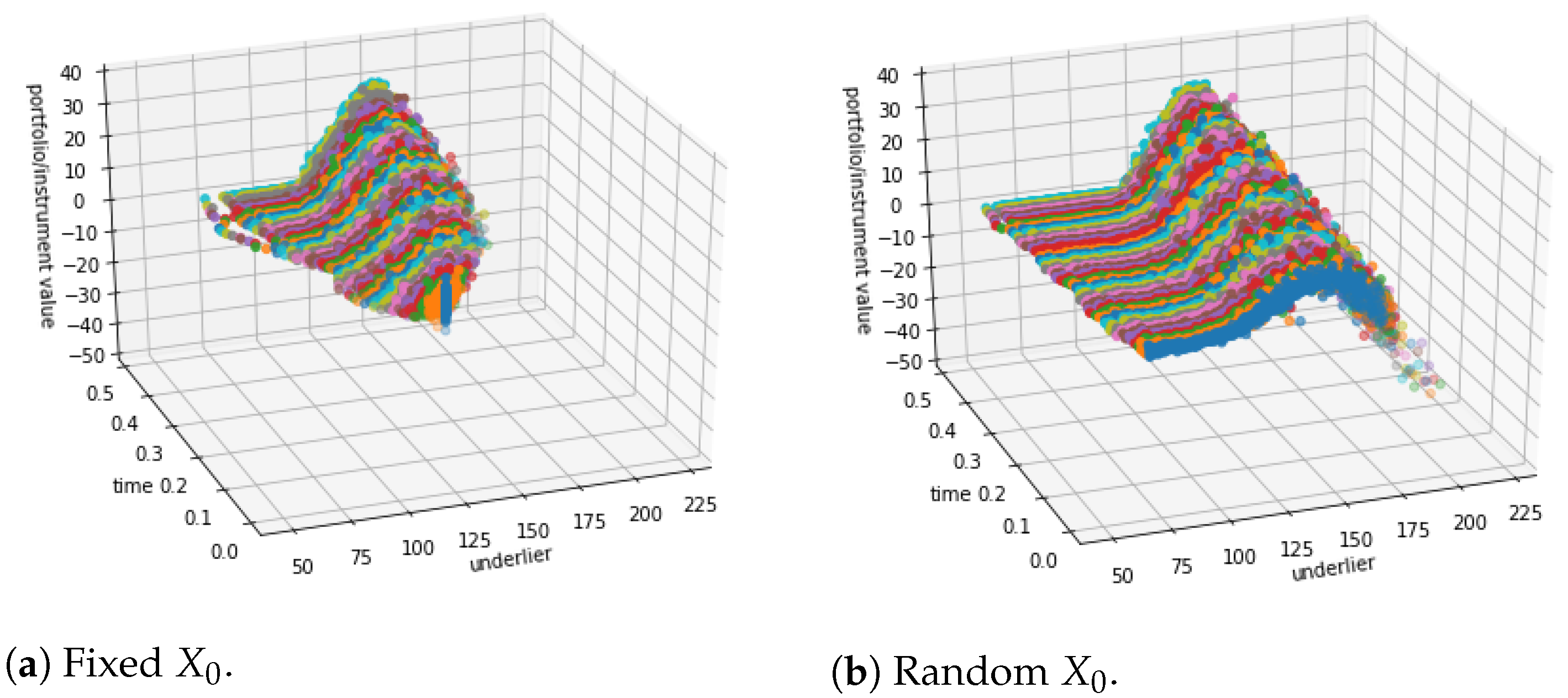
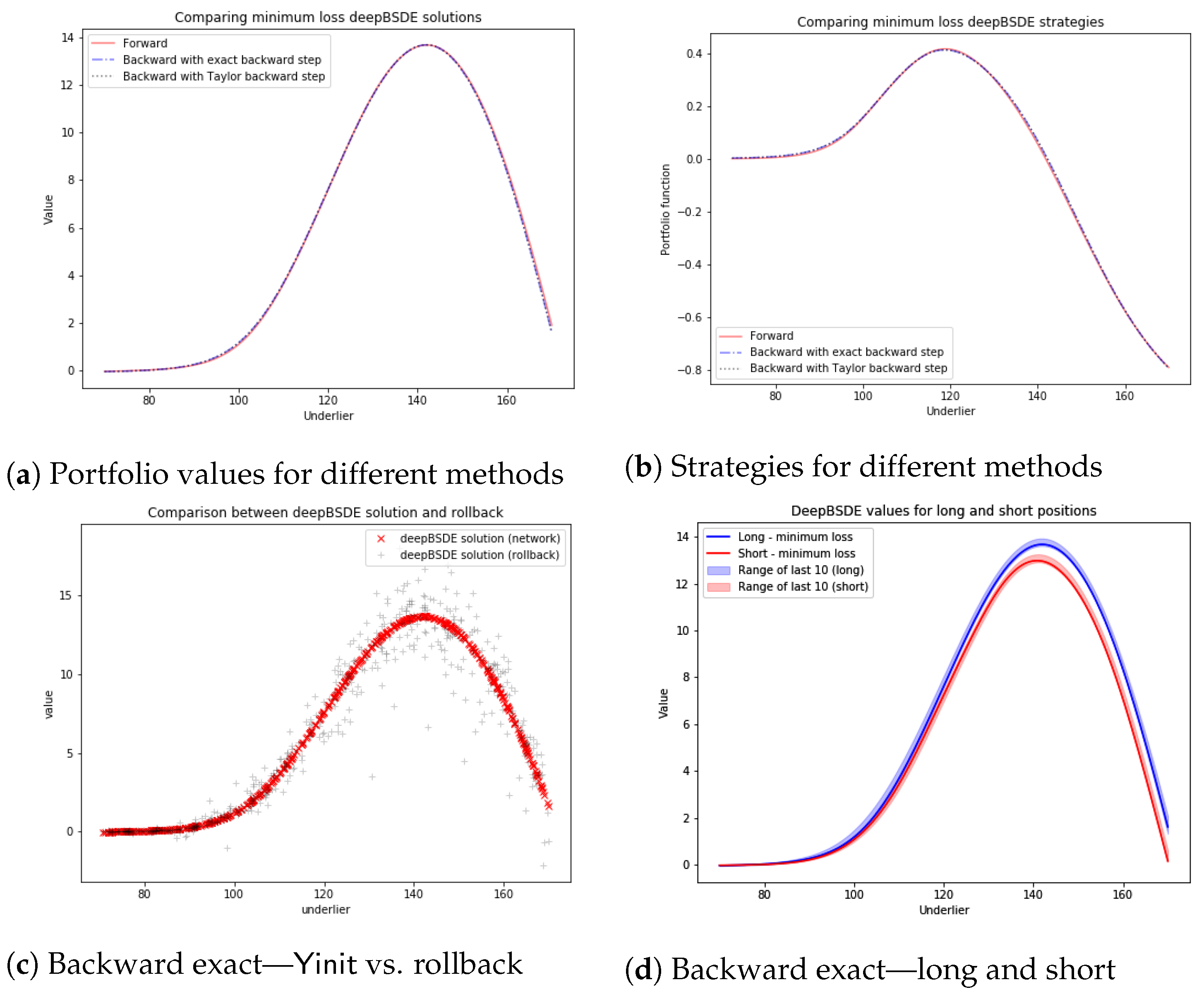
Figure 3 shows the Y path values for fixed X 0 (on the left) and for uniform random X 0 (on the right) for the long call combination. Notice that the random X 0 variant covers much more of the solution surface. Figure 4 shows initial Yinit network results vs. rollback, minimal loss solution and the range of the 10 last validation solutions for long and short, and solution and strategy from different methods. We see that the solutions from different deep BSDE (including Taylor vs. exact step) are close to each other, and the strategies are also rather similar, with the forward strategy slightly different but close.

4.2. Straddle

(Forsyth and Labahn 2007, Table 1 on page 28 in hjb.pdf) picked σ = 0.3 , μ = r b = 0.05 , and r l = 0.03 . We used 100 time-steps (one of the numbers of time-steps for which results are given in tables in Forsyth and Labahn (2007)). The strike for the straddle is 100. We used various batch sizes, prescaling, Adam with default parameters and exponentially decaying learning rate, two hidden layers with d i m + 10 = 11 neurons, and activation function Softplus for the first two layers and then identity on the output layer, as in the call combination case.
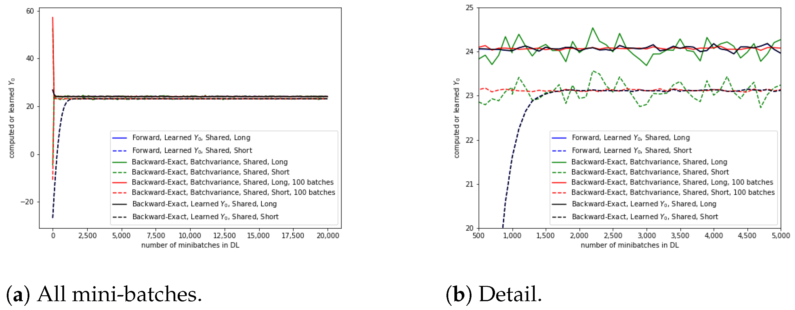
We first consider the fixed X 0 case. Like Forsyth and Labahn (2007), we pick X 0 to be 100. In Figure 5, we plot Y 0 estimates and parameter for different backward and forward methods for a certain range of mini-batches, showing the behavior once the methods have converged to a region where the mini-batch size limits how well the loss function is approximated (and thus the results vary within a range). We see that the method that learns the Y 0 parameter initially converges more slowly (which the lower price converging even more slowly than the upper price) than the batch-variance methods. However, once close to true value, its convergence is smoother and better than the batch-variance methods—and it varies less. Computing the mean over 100 mini-batches rather than over one leads to a faster and smoother convergence of the initial value for the batch-variance variants.
We use this example to visualize the details of the pathwise backward methods. We set π to the strategy obtained after optimizing over 100, 1000, and 20,000 mini-batches using the exact backward step with the batch-variance variant for fixed X 0 . Using these strategies, we generate many samples from the rollback random variable Y 0 π and show them in Figure 6. The optimization starts with a π DNN with random weights and biases. In the beginning of the optimization, the strategy cannot control the distribution of the rollback well yet, but it slowly reduces the distribution’s variance, making it (approximately) unimodal. After batch 100, the strategy for the short position already creates a unimodal distribution for the rollback, while the strategy for the long position still results in a distribution that is bimodal and more spread out. After batch 1000, both strategies result in unimodal and narrowing distributions. After batch 20,000, the strategies are even narrower and more peaked, with clearer separation between short and long.
In Figure 7, we show the distribution of batch means for freshly generated mini-batches, now only for the policy from the 20,000th mini-batch. This distribution is much narrower and clearly separated between long and short. For comparison, we also plotted the mean over all generated mini-batches.
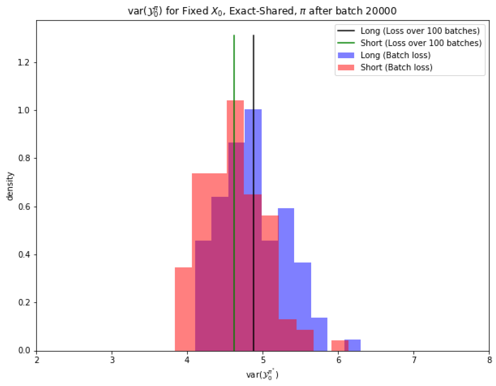
In Figure 8, we show the distribution of batch losses for freshly generated mini-batches, again only for the policy from the 20,000th mini-batch. For comparison, we also plotted the average loss over all generated mini-batches. We can see that the losses are similarly distributed for short and long positions. To estimate the loss very well from a single mini-batch, one would need a batch size that is 10 or 100 times larger. However, using stochastic gradient descent approaches has the advantage of implicit regularization and avoidance of local minima.
Figure 9 shows loss curves over five independent runs started from different seeds. Crosses indicate losses approximated by single mini-batches; black shows loss approximations averaged over ten mini-batches, with red showing ranges implied by ten mini-batches. While the behavior under different seeds is different in the beginning, it becomes very similar and lies in the same range once the optimization through stochastic gradient descent or Adam progresses more and more. The curves all go through the same phases—an initial fast decrease which subsequently slows down and then slowly decreases and stabilizes once the loss reaches the magnitude of estimation and stochastic gradient noise.
One can similarly extract, visualize, and study the distribution of the rollbacks and their means and losses defined on them (with respect to batch mean, with respect to a learned mean, or with respect to an externally given reference mean). In the noisy region where the loss has stabilized up to noise, the distribution of the rollbacks, means, and losses during the stochastic gradient descent method or Adam method starts to resemble the distribution under one (randomized or deterministic) policy but with much larger sample size. This actually means that if we work with the distribution of rollbacks, means, or losses over a sequence of mini-batches from the optimization from that noise region, we will obtain results corresponding to methods with larger samples and mini-batch sizes, allowing us to obtain quite accurate results despite the relatively small mini-batch size (such as 128, 256, or 512). Since the loss estimate from a single mini-batch is not very accurate, selecting the strategy to be from the mini-batch with the smallest loss estimate does not necessarily result in picking the strategy with the smallest actual loss. However, one can pick several candidate strategies and estimate the loss more accurately and then select the one with the smallest accurate loss or use an ensemble from some with small accurate losses. Since our results (mean or range over mini-batches during optimization) agree well with the range of results given by Forsyth and Labahn (2007), we do not do so here, but we plan to do so in future work.
We compare our lower and upper price against the results given in (Forsyth and Labahn 2007, Tables 2 and 3) in Table 1. The results are very close to each other. Since Forsyth and Labahn use a PDE method, they report results for a certain number of space steps, while our method does not discretize space. They report results for higher numbers of space steps (and an equally higher number of time-steps) which are even closer to our results, but the different number of time-steps does not allow definite conclusions.
In Table 2, we report the results over five different random seeds. One can see that the price across seeds varies within an interval around the prices given in Forsyth and Labahn. The particular seed does not impact the price a lot. The range of prices over mini-batches in the optimization in the noise region provides estimates that are consistent with estimates across different random seeds.
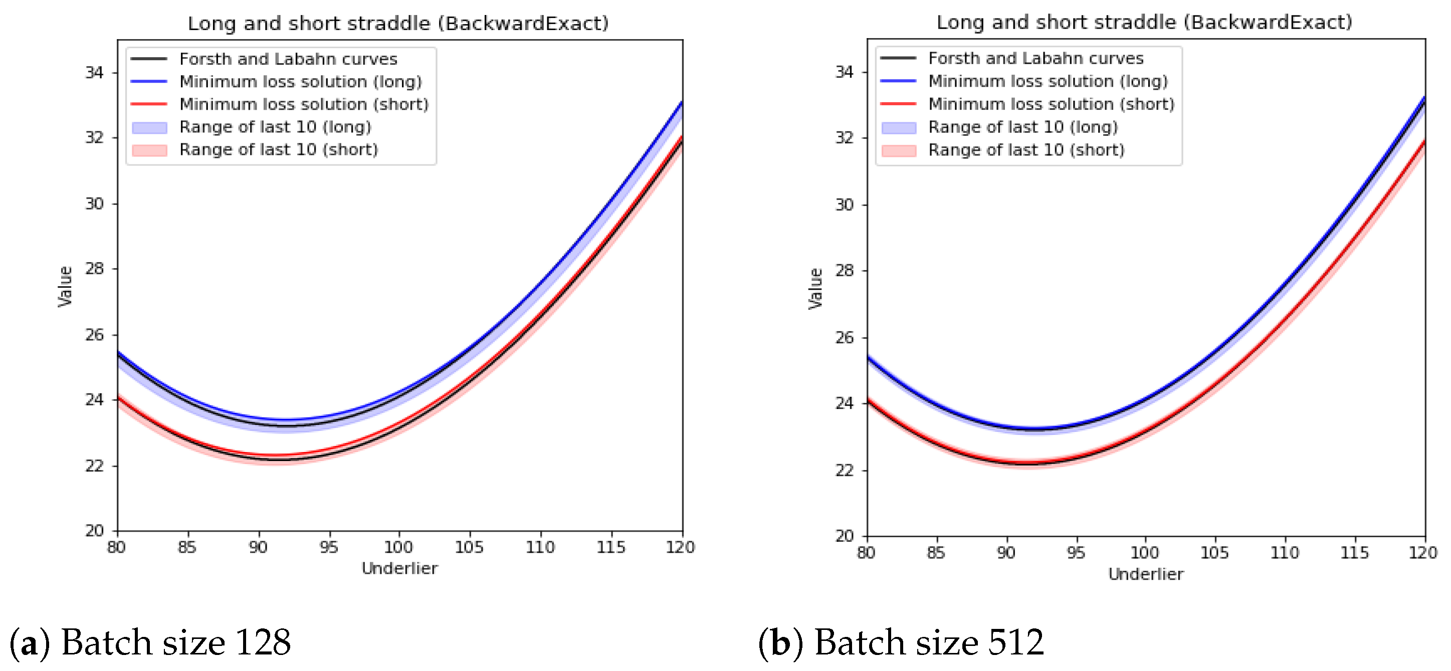
For the random X 0 case, we pick X 0 uniformly within the range [ 50 , 150 ] but plot results within the range [ 80 , 120 ] . We saved and discretized Figure 1 from (Forsyth and Labahn 2007, Figure 1) (the hjb PDF version), extracted relative coordinates for the points on the curve and converted them to values, and plotted them as curves in the figures (curves shown in black).
Figure 10 shows comparisons of the backward exact deep BSDE method (both minimum loss solution and range of last 10) against the curves from (Forsyth and Labahn 2007, Figure 1), while Figure 11 shows comparisons of different deep BSDE methods against each other. It can be seen that the curves from (Forsyth and Labahn 2007, Figure 1) are within the range for both batch sizes and that the different methods mostly agree, although somewhat more so for batch size 512.6 Similarly to before, exact vs. Taylor step only has minimal impact.

5. Conclusions

We first introduced FBSDE for general nonlinear problems, with particular details for the differential rates problem, time-discretized them, and then derived exact solutions and Taylor approximations for the backward step equation. We then quickly described the pathwise forward and backward deep BSDE approaches that we consider—both the batch-variance variant already described in the literature and also the novel initial variable and network versions; the last one is for random X 0 . Then, we applied these methods for the differential rates problem for the call combination case from Han et al. (2018) and for the straddle case from Forsyth and Labahn (2007). We compared the results for a case with fixed X 0 and for a case with varying X 0 with the results from Forsyth and Labahn (2007) and saw that they agree well with Forsyth and Labahn (2007) and each other.
The deep BSDE methods described in this paper use a very different approach from the PDE methods in Forsyth and Labahn (2007), but they give results that agree well with those published there. This makes us confident that these methods can be used to generically and efficiently approximate solutions to such nonlinear pricing problems, using relatively small batch sizes such as 128, 256, or 512.

6. Disclaimer

Any opinions, findings and conclusions or recommendations expressed in this material are those of the authors and do not necessarily reflect the views of Wells Fargo Bank, N.A., its parent company, affiliates, and subsidiaries.

Author Contributions

Conceptualization, Y.Y., N.G. and B.H.; methodology, Y.Y., N.G. and B.H.; software, Y.Y., N.G. and B.H.; validation, Y.Y., N.G. and B.H.; formal analysis, Y.Y., N.G. and B.H.; investigation, Y.Y., N.G. and B.H.; writing—original draft preparation, Y.Y., N.G. and B.H.; writing—review and editing, B.H.; visualization, Y.Y., N.G. and B.H.; supervision, B.H.; project administration, B.H.; All authors have read and agreed to the published version of the manuscript.

Funding

This research received no external funding.

Data Availability Statement

Not applicable

Acknowledgments

The authors would like to thank Orcan Ogetbil, Daniel Weingard, and Xin Wang for proof reading drafts and giving helpful feedback; Vijayan Nair for discussion regarding methods, presentation, and results, as well as for reviewing the paper; and Agus Sudjianto for supporting this research. They would also like to thank Dan Pirjol for suggestions and recommendations that helped improve the readability and presentation of this manuscript.

Conflicts of Interest

The authors declare no conflict of interest.

Notes

1
Set Z t = Π t T σ ( t , X t ) and f ˜ ( t , X , Y , Z ) = f ( t , X , Y , σ ( t , X t ) T Z t T ) . Then, (Pardoux 1998, Theorem 2.2) with this Z t and f ˜ shows that one can construct a solution Y t and Z t of the BSDE from a classical C 2 , 1 solution of a corresponding PDE and a solution X t . Rewriting the PDE and BSDE in terms of Π t T instead of Z t and using function f rather than f ˜ gives the form reported below. For the opposite direction, (Pardoux 1998, Theorem 2.4) shows how a solution Y t of the BSDE (corresponding to a X that starts at x at time t) gives a continuous function u ( t , x ) , which is a viscosity solution of the corresponding PDE.
2
In general, the terminal condition could be given as a random variate G T that is measurable with respect to the information available of time T (i.e., the sigma algebra generated by X t with t T ). The FBSDE approach then will be more general than the PDE approach. If there is an exact (or approximate) Markovianization with a Markov state M t , the strategy Π t and the solution Y t would in general be functions π ( t , M t ) and u ( t , M t ) of that Markov state. We only treat the usual final value case here.
3
There are many introductions into DL, DNN, and common forms of DNN. For a minimal one geared towards deep BSDE, see Hientzsch (2021).
4
This is actually the expectation of the conditional variance var ( Y 0 π | X 0 ) over the distribution of X 0 .
5
Here, we consider the 1-dimensional case, while Han and Jentzen (2017) consider the 100-dimensional case.
6
Notice that (Forsyth and Labahn 2007, Figure 1) do not give the number of space or time-steps used for their plot.

References

  1. Forsyth, Peter A., and George Labahn. 2007. Numerical methods for controlled Hamilton-Jacobi-Bellman PDEs in finance. Journal of Computational Finance 11: 1–44. Available online: https://cs.uwaterloo.ca/~paforsyt/hjb.pdf (accessed on 15 March 2023). [CrossRef] [Green Version]
  2. Ganesan, Narayan, Yajie Yu, and Bernhard Hientzsch. 2022. Pricing barrier options with deep backward stochastic differential equation methods. Journal of Computational Finance 25. Available online: https://ssrn.com/abstract=3607626 (accessed on 15 March 2023). [CrossRef]
  3. Han, Jiequn, and Arnulf Jentzen. 2017. Deep learning-based numerical methods for high-dimensional parabolic partial differential equations and backward stochastic differential equations. Communications in Mathematics and Statistics 5: 349–80. [Google Scholar]
  4. Han, Jiequn, Arnulf Jentzen, and Weinan E. 2018. Solving high-dimensional partial differential equations using deep learning. Proceedings of the National Academy of Sciences 115: 8505–10. [Google Scholar] [CrossRef] [PubMed] [Green Version]
  5. Hientzsch, Bernhard. 2021. Deep learning to solve forward-backward stochastic differential equations. Risk Magazine. February. Available online: https://ssrn.com/abstract=3494359 (accessed on 15 March 2023).
  6. Huré, Côme, Huyên Pham, and Xavier Warin. 2020. Deep backward schemes for high-dimensional nonlinear PDEs. Mathematics of Computation 89: 1547–79. [Google Scholar] [CrossRef] [Green Version]
  7. Liang, Jian, Zhe Xu, and Peter Li. 2021. Deep learning-based least squares forward-backward stochastic differential equation solver for high-dimensional derivative pricing. Quantitative Finance 21: 1309–23. Available online: https://ssrn.com/abstract=3381794 (accessed on 15 March 2023). [CrossRef]
  8. Mercurio, Fabio. 2015. Bergman, Piterbarg, and beyond: Pricing derivatives under collateralization and differential rates. In Actuarial Sciences and Quantitative Finance. Berlin: Springer, pp. 65–95. Available online: https://ssrn.com/abstract=2326581 (accessed on 15 March 2023).
  9. Pardoux, Étienne. 1998. Backward stochastic differential equations and viscosity solutions of systems of semilinear parabolic and elliptic PDEs of second order. In Stochastic Analysis and Related Topics VI. Berlin: Springer, pp. 79–127. [Google Scholar]
  10. Raissi, Maziar. 2018. Forward-backward stochastic neural networks: Deep learning of high-dimensional partial differential equations. arXiv arXiv:1804.07010. [Google Scholar]
  11. Wang, Haojie, Han Chen, Agus Sudjianto, Richard Liu, and Qi Shen. 2018. Deep learning-based BSDE solver for LIBOR market model with application to bermudan swaption pricing and hedging. arXiv arXiv:1807.06622. Available online: https://ssrn.com/abstract=3214596 (accessed on 15 March 2023). [CrossRef]
  12. Warin, Xavier. 2018. Nesting Monte Carlo for high-dimensional non-linear PDEs. Monte Carlo Methods and Applications 24: 225–47. [Google Scholar] [CrossRef] [Green Version]
Figure 1. Computational graph for the entire method with initial network.
Risks 11 00061 g001
Figure 2. Loss function over 20,000 mini-batches for long call combination for batch-variance method with exact backward step. Loss functions for the other variants look very similar. Batch size 512.
Risks 11 00061 g002
Figure 3. Y path values at 20,000 mini-batches for the batch-variance version with exact backward step (other variants look very similar) for long call combination with fixed X 0 on the left and initial network version with random X 0 on the right. Notice the much smaller coverage for fixed X 0 . Batch size 512.
Risks 11 00061 g003
Figure 4. Call combination: results for random X 0 . Batch size 512. Panels (ac) show results for a long position. (d) shows results for both long and short positions.
Risks 11 00061 g004
Figure 5. Y 0 estimates or parameters for the straddle case—all 20,000 mini-batches (a) and detail (b). Exact backward step. (Batch size 256). The results for Taylor backward step look very similar.
Risks 11 00061 g005
Figure 6. Distribution of the rollback Y 0 π for strategies of certain batches in the optimization. Straddle. Backward method with exact backward step. Single DNN for π . Batch size 512.
Risks 11 00061 g006
Figure 7. Distribution of batch means of the rollback Y 0 π for the strategies after the 20,000th batch in the optimization. Straddle. Backward method with exact backward step. Single DNN for π . Batch size 512.
Risks 11 00061 g007
Figure 8. Distribution of batch losses for the rollback Y 0 π for the strategies after the 20,000th batch in the optimization. Straddle. Backward method with exact backward step. Single DNN for π . Batch size 512.
Risks 11 00061 g008
Figure 9. Loss function over 20,000 mini-batches for the short and long straddle for batch-variance method with exact backward step with a single DNN for π for five independent realizations. Behavior is very similar for other variants.
Risks 11 00061 g009
Figure 10. Yinit ( X 0 ) for two batch sizes and backward exact step plotted against Forsyth and Labahn curves from (Forsyth and Labahn 2007, Figure 1).
Risks 11 00061 g010
Figure 11. Yinit ( X 0 ) for various methods for two batch sizes.
Risks 11 00061 g011
Table 1. Different pricers. * Means that Taylor is different by 0.01. Fixed X 0 . Y 0 range over every 100 in the last 1000 in parentheses. Middle of range as price.
MethodUpper PriceLower Price
Results from Forsyth and Labahn-101 nodes
Fully Implicit HJB PDE (implicit control)24.0223.06
Crank–Nicolson HJB PDE (implicit control)24.0523.09
Fully Implicit HJB PDE (pwc policy)24.0123.07
Crank–Nicolson HJB PDE (pwc policy)24.0723.09
Forward deep BSDE—20,000 batches, size 256
Learned Y 0 (shared)24.06 (23.99–24.14)23.10 (23.02–23.17)
Learned Y 0 (separate)24.07 (24.01–24.12)23.10 (23.06–23.15)
Backward deep BSDE—20,000 batches, size 256
Batch variance/1 (shared)24.14 (23.98–24.30)23.19 (23.00–23.37)
Batch variance/100 (shared)24.08 (24.06–24.09)23.13 (23.09–23.16)
Batch variance/1 (separate)24.06 (23.94–24.19 *)23.10 (22.95–23.25)
Batch variance/100 (separate)24.07 (24.06–24.09 *)23.12 (23.10–23.13)
Learned Y 0 (shared)24.06 (23.99–24.14)23.10 (23.02–23.17)
Learned Y 0 (separate)24.06 (24.01–24.11 *)23.10 (23.06–23.15)
Table 2. Impact of random seed. Fixed X 0 . Exact backward step. Range of price over seeds. Y 0 range over every 100 in the last 1000 in parentheses.
MethodUpper PriceLower Price
Results from Forsyth and Labahn—101 nodes
Fully Implicit (implicit control)24.0223.06
Crank–Nicolson (implicit control)24.0523.09
Fully Implicit (pwc policy)24.0123.07
Crank–Nicolson (pwc policy)24.0723.09
Backward deep BSDE—20,000 batches, size 512, five seeds
Batch variance/1 (shared)24.02–24.08 (23.87–24.29)23.06–23.12 (22.91–23.33)
Batch variance/100 (shared)24.06–24.07 (24.03–24.09)23.11–23.12 (23.09–23.15)
Disclaimer/Publisher’s Note: The statements, opinions and data contained in all publications are solely those of the individual author(s) and contributor(s) and not of MDPI and/or the editor(s). MDPI and/or the editor(s) disclaim responsibility for any injury to people or property resulting from any ideas, methods, instructions or products referred to in the content.