Abstract
We study the convergence of the binomial, trinomial, and more generally m-nomial tree schemes when evaluating certain European path-independent options in the Black–Scholes setting. To our knowledge, the results here are the first for trinomial trees. Our main result provides formulae for the coefficients of and in the expansion of the error for digital and standard put and call options. This result is obtained from an Edgeworth series in the form of Kolassa–McCullagh, which we derive from a recently established Edgeworth series in the form of Esseen/Bhattacharya and Rao for triangular arrays of random variables. We apply our result to the most popular trinomial trees and provide numerical illustrations.
1. Introduction
In this article, we assume that the stock price follows the Black–Scholes model, that is,
where is the drift and is the volatility. In order to price options, the martingale measure is introduced under which is replaced by the risk-free interest rate r. After the Black–Scholes model was introduced, the binomial model appeared and it is shown by () that the European call and put option price , calculated by their binomial model, converges to the Black–Scholes price as the number of periods (or time steps) . Later (see the literature discussion below), scholars studied the rate of the convergence of to and found that for certain binomial models there was a bounded coefficient , such that . Now, trinomial models have been studied by many authors. However, as far as we are aware, there are no similar results for trinomial prices. The main objective of this paper is to fill this gap. In fact, our study comprises general self-similar m-nomial models, that is, at any positive time step, the stock price changes to one of m prices at the next period, where the mechanism and probabilities of these changes are independent of the value of the stock and the time of the change may depend on n, which is the number of periods. The trinomial case corresponds to . m-nomial models, where , have been rarely used, but it turned out that our results were as easily proved for general m as for . The trees we study are recombining, as models which are not recombining are not interesting from the computational point of view. As far as we know, the models we study include all self-similar binomial and trinomial models studied in the literature, except the somewhat pathological cases, where the convergence of call and put option prices occurs at a speed of only .
In this paper, under general conditions which ensure that the moments of the stock price in the m-nomial model behave like the moments in the Black–Scholes model, we demonstrate in Theorem 1 that the price of a European put in the m-nomial model satisfies the relation
where is the Black–Scholes price and is a bounded sequence which we determine explicitly. A similar result for calls is obtained by using a put-call parity. Of course, depends on the particular model being used. For digital options, we obtain an analogous formula, where, however, the coefficient of is not zero. Note that we obtain the results of () as special cases.
The proof of Theorem 1 uses an Edgeworth series. () were the first to extend the Edgeworth series to triangular arrays of random variables, and they applied their results to binomial models. Here, we demonstrate that their analysis can also be applied to m-nomial models. The form of Edgeworth series used by Bock and Korn was inspired by () and (). We are able to simplify their expansion using the ideas of ().
In the case of European path-independent options, the following results have been obtained for binomial trees. If the price of an option calculated in a tree model with n time steps converges to the Black–Scholes price of the same option, we say that there exists an asymptotic expansion of the error of order in the powers of if there exist bounded coefficients , such that
for some integer . Using Skorokhod embedding, () found an explicit expansion of the error of order for European path-independent options subject to a general class of payoff functions, but in the specific case of where the discounted process satisfies the Cox–Ross–Rubinstein (CRR) scheme. () used an integral expression for the price of call options in a general class of binomial models to demonstrate how an expansion in the powers of of the price of call options can be obtained up to an arbitrary order of using a Computer Algebra System (CAS) such as Maple. () introduced a general class of binomial models with an additional drift parameter that smooths the convergence of the option prices. Using a result by (), they provided an explicit formula for the coefficient of and in the expansion of the error for digital call and call options. In (), Joshi showed that when n is odd and the terminal layer of the tree is centered around the strike, the coefficients in the expansion (1) of European call and put options are independent of n. In a follow-up paper, () constructed binomial trees with an arbitrarily fast convergence for vanilla European options. () found an expression for the optimal drift in Chang and Palmer’s general class of binomial models. Using a localization of the error, () found an explicit expansion of the error of order in the case of general payoff functions for the general class of binomial models introduced by Chang and Palmer. Using the expansion in (), () showed how the drift can be chosen to reach an arbitrarily fast convergence in Chang and Palmer’s model. () developed a formula for the Edgeworth expansion of the cumulative distribution of
for independent and identically distributed -valued triangular arrays , , of random variables with mean , and they used it to improve the convergence of option prices. Using the expansion in (), () found an explicit expression for the coefficient of (the coefficient of being zero) in the expansion in powers of for the price of a European put option calculated using a two-parameter non self-similar split tree introduced by (), which was designed to improve the convergence for the American put option.
To further motivate this paper, let us mention that, due to their simplicity and flexibility, binomial and multinomial trees are used in the pricing of a broad class of options such as barrier options (; ; ), lookback options (; ; ), Asian options (; ; ), Parisian and ParAsian options (). Binomial and multinomial trees are also used for pricing options in several models, such as Levy models (), stochastic volatility models () and regime switching models (; ). In (), the discrete Malliavin calculus is developed for option sensitivity with binomial tree models, and spectral binomial trees are used to price double barrier options. A discrete cosine transform approach for the binomial tree is developed in (). In spite of (, , ; ; ), it remains an open problem to establish a sharp convergence speed for the price of the American put options evaluated in a binomial tree approximation of the Black–Scholes model. In (), it is pointed out that “a particularly interesting work would be to provide an error analysis for numerical methods based on trees for general diffusion models”. The techniques developed for vanilla options in the Black–Scholes model have often been central in papers dealing with more complex options, and we believe that Edgeworth price expansions based on moments and cumulants, such as the one developed in this paper, will find applications in a future work dealing with more complex options.
Now, we summarize the contents of the paper. In Section 2, we define m-nomial models and find an expression for the m-nomial prices of put options in terms of the prices of two digital put options using a change of numeraire. In Section 3, we state our main theorem, Theorem 1, providing the coefficients of and in the expansion (1) for digital put and standard put options. Next, in Section 4, we verify that our result coincides with the result of () for binomial trees. Then, we use Theorem 1 to find expressions for the coefficients of and in the expansion of the error in four well-known trinomial models, and we run some simulations to support our result numerically. In Section 5, we prove Theorem 1. The proof is based on a theorem (Theorem 2) for the expansion of the m-nomial prices of digital put options. Theorem 2 is proved in Section 6. Theorem 2 follows in turn from Theorem 3, which is proved in Section 7. Theorem 3 derives from the Edgeworth series in the form of (), using the result of (). The proof of Theorem 3 depends on the technical results that we put in the Appendix A.
2. -Nomial Models
First, we define what we mean by an m-nomial model.
Definition 1.
Given initial stock price and maturity , we say that , , with is an n-period m-nomial model if at time , the price can take any of the m values with
where . The condition implies that . We further assume that so that . The probabilities that satisfy . We denote such a model by where . The model is risk neutral if
Note that does not depend on i and this ensures that the tree is recombining. This is obviously satisfied when , that is, for binomial models, and it seems to be satisfied for all self-similar trinomial models in the literature. Note that once the are determined, there may not exist probabilities such that and if they do exist, they may not be unique (except in the binomial case). For example, in the trinomial case , such probabilities exist if and only if and can be chosen as any number in the interval
with
When the probabilities are risk neutral, there are no arbitrage opportunities in the m-nomial model. However, except in the binomial case, the risk-neutral probabilities are not unique and an option does not have a uniquely defined price. In any case, relative to a given set of probabilities, we take the price of an option with payoff , where is the terminal stock price, to be , where the expectation is with respect to the given probabilities, and we do this even when the probabilities are not risk neutral.
In the risk neutral case, put–call parity holds with the above definition of the price since the payoff to a long call and a short put with exercise price K and maturity T is and, under risk neutrality, . Thus, we can derive the price of a call option from that of a put option.
Next, we demonstrate that when the probabilities are risk neutral, the formula for the m-nomial price of a put option can be written as a combination of the formulas for two digital put options. In the Black–Scholes world with initial stock price , volatility and interest rate r, the price of a put option with strike K and maturity T is given by
where is the standard normal cumulative distribution function and
Here, is the probability that is under the risk neutral measure so that is the price of a digital put with strike K. is the probability that under the stock measure and similarly is the price of a digital put with strike K under the stock measure. We show that a similar result holds for a risk-neutral m-nomial model. Our argument adapts Cox and Rubinstein’s argument in () for the binomial model.
The possible values of the terminal stock price are
where , and . Thus, the terminal stock prices are
where . Let be the probability of reaching the price . Then, the price of a put option with strike K is
where is such that
Then
Now
where . Then
where
Note that
and that
so that the ’s can be thought of as the stock measure corresponding to the risk neutral measure defined by the , that is under the probability measure defined by we have Then
where
Note that is the probability of arriving at a stock price under the risk neutral probabilities , whereas is the probability of arriving at a stock price under the probabilities . Thus, the problem of pricing a put option is reduced to pricing two digital put options.
3. The Main Theorem
Now, we state our main theorem. We assume we are in the Black–Scholes world with an initial stock price , volatility and interest rate r, and that the options under consideration have maturity T. Then, we require the following hypotheses on our m-nomial model with parameters .
(H1): is bounded, has a positive (>0) limit and
(H2): Define as the random variable which takes the value with probability , . Note that is bounded. Then, we assume
where , , , , are bounded functions of n, and where we observe that .
Remark 1.
Note that in our m-nomial model, we want to be an approximation to , where is the stock price under the Black–Scholes model, when the stock price at time 0 is , the interest rate is r and the volatility is σ. Thus, we want to be an approximation to , which is normally distributed with mean and variance . Then,
Under (H1), it can be demonstrated that (H2) is equivalent to the condition that all moments of the terminal stock price in the m-nomial model converge at a rate of to the corresponding moments of the terminal stock price in the Black–Scholes model.
Now, we state the main theorem.
Theorem 1.
Suppose is an n-period m-nomial model with parameters , time steps and initial stock price for which (H1) and (H2) hold. We define the price of an option in this model with payoff to be , where the expectation is taken with respect to the measure defined by the probabilities . Then,
(i) the price of a digital put option with strike K and maturity T in the n-period m-nomial model satisfies
where is the Black–Scholes price, is the standard normal density function,
and
(ii) If, in addition, the model is risk-neutral, the price of a put option with strike K and maturity T in the n-period m-nomial model satisfies
where is the Black–Scholes price and
The price of a call option satisfies the same equation.
Remark 2.
Note that , so that
where . Thus, describes the position of the strike relative to the terminal stock prices (see (4)). Since, in general, oscillates between 0 and 1, the quantity also oscillates.
Remark 3.
The risk neutral condition in (ii) is not needed. Under the hypotheses of the theorem, we find that
where . Then, it turns out that, for the put price, (ii) still holds if we add to the , which would be obtained if the model were risk neutral. For the call price, an additional term has to be added to .
4. Verification of the Result
We test our result in two ways. First, we check that in the case of the flexible binomial model of (), (which includes the CRR model as a special case), our results reduce to those in Chang and Palmer. Then, we apply Theorem 1 to four trinomial models and test our result numerically on these trinomial models.
4.1. Comparison with Chang and Palmer’s Binomial Model
First, we compare our results with the binomial model in Chang and Palmer, where in their notation,
The authors considered digital calls but, by modifying their proof, we can demonstrate that the binomial price of a digital put satisfies
where
and is
In this risk neutral model, (H1) and (H2) are satisfied with and
where
Applying Theorem 1, we observe first that Some algebra yields
This coincides with in the Chang–Palmer result. Thus, in the case of digital puts, Theorem 1 gives a result consistent with that of Chang and Palmer.
For the Chang–Palmer model, applying put–call parity to the Chang–Palmer result for calls, we find that after some rearrangement, the price of a put option satisfies
where is as in (7) and
Now, from Theorem 1, since, as above, ,
where, again after some algebra, we find that
Again, this coincides with in the Chang–Palmer result. Thus, also in the case of puts, Theorem 1 gives a result consistent with that of Chang and Palmer.
4.2. Application of Theorem 1 to Trinomial Models
Next, we calculate and in Theorem 1 for five trinomial (that is, ) models, the first four of which are risk-neutral. These models satisfy (H1) and (H2). In fact, , , , are constants and constant + , all of which have the consequence that and are constants. In all these models, we write
(1) First, we study ’s () equal probability tree, where
with , and . For this model, we find that
where and hence that
(2) Next, we study ’s () fourth-order moment matching model, where the first four moments of match the moments of in the Black–Scholes model. In this model,
where , and . We find that
and hence that
(3) Next, we study the adjusted trinomial tree (), where the tree is centered on the strike in the log space. In this model, the probabilities , and are defined as in the previous model but now and
We find, as in the previous model, that
and hence that
(4) Next, we study Boyle’s tree (), with parameter , in which
where and . Then
and hence
(5) Finally, we study the Kamrad–Ritchken model () with parameter , in which
This model is not risk neutral, since
where
All other hypotheses of Theorem 1 are satisfied with
For the digital put, we find that is
For the put option, it follows from Remark 3 that is
Notice that all values coincide for models (2) and (3). When , the moments in Boyle’s model match those in these models up to negligible terms, so that and reduce to those in models (2) and (3).
4.3. Numerical Results for the Trinomial Models
Finally, numerical results for the trinomial models described above are displayed in Figure 1, Figure 2, Figure 3 and Figure 4 when , , , and . We label Tian’s equal probability model as ‘EqualProb’, Joshi’s adjusted trinomial model as ‘Adjusted’, Boyle’s model with parameter as ‘Boyle’, Kamrad-Ritchken’s model with parameter as ‘KR’, and Tian’s fourth-order moment matching model as ‘Tian4’.
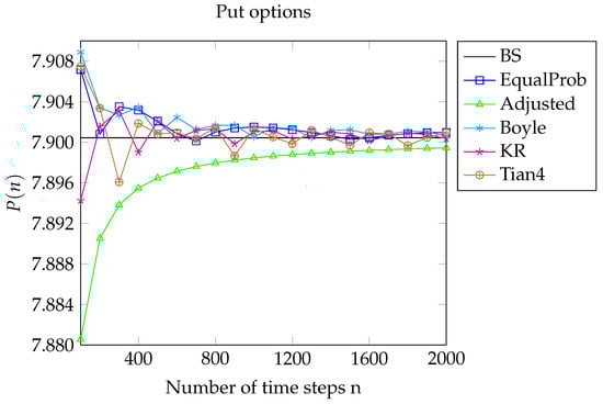
Figure 1.
Here, , , , and . We plot the prices of put options in various trinomial models against the Black–Scholes price .
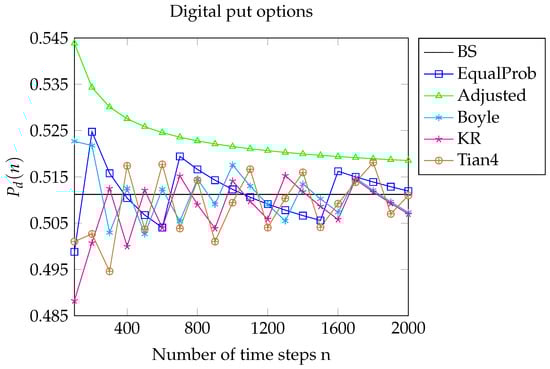
Figure 2.
Here, , , , and . We plot the prices of digital put options in various trinomial models against the Black–Scholes price .
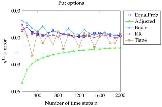
Figure 3.
Here, , , , and . For the put, the Black–Scholes price . is the n-period price calculated by various models, and We expect error to be bounded and this appears to be the case.
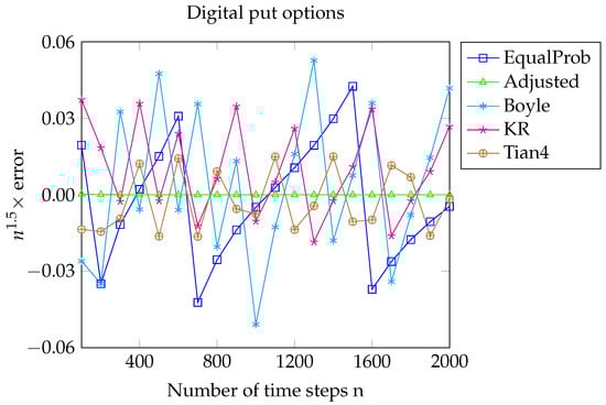
Figure 4.
Here, , , , and . For the digital put, the Black–Scholes price . is the n-period price calculated by various models, and We expect error to be bounded and this again appears to be the case.
For the put, the Black–Scholes price , and we denote by the n-period price calculated in the trinomial models. For the digital put, the Black–Scholes price , and we denote by the n-period price calculated in the trinomial models. Letting , Figure 1 illustrates the convergence of to , while Figure 2 illustrates the convergence of to .
Figure 1 and Figure 2 show that the price’s convergence to the Black–Scholes limit for Joshi’s adjusted model is far less oscillatory than that of the other models. This is because , so that the strike K is the terminal node of the tree. Consequently, , because and so that . It follows that the coefficients of and in the expansions of the prices are constant. As a result, the convergence is smoother than it is for the other models, where oscillations triggered by cause the coefficients of and in the price expansion to oscillate.
For the put option, we define ‘error’ as
For the digital put option, we set
We expect error to be bounded and this seems to be the case, as illustrated in Figure 3 for the put option and in Figure 4 for the digital put option.
Figure 3 and Figure 4 show that the values of error for Joshi’s adjusted model are far less oscillatory than those for the other models. This suggests that the coefficient of in the price expansion is constant. In the case of the digital put, the coefficient appears to be 0. This could be verified using Edgeworth expansions with more coefficients. We leave this to the interested reader.
5. Proof of Theorem 1
The main tool in the proof is the following theorem, which gives an Edgeworth expansion for the cdf of the terminal stock price in an m-nomial model. We defer the proof to later. First, we define an Edgeworth expansion.
Let , , be any sequence of sequences of real numbers such that for all n. Set . This notation is used because usually corresponds to a variance. Then, for each integer , the Edgeworth expansion is defined as
where is the standard normal cdf and , , is defined by the relation
Clearly, , . Note, we can also write
where is the standard normal pdf and is the jth Hermite polynomial. This is a consequence of the fact that
Theorem 2.
Suppose is an n-period m-nomial model with parameters , time steps and initial stock price for which (H1) holds and . Let be the Bernoulli number. Denote by the jth cumulant of , and set
where
Then, for every integer , and every ,
Remark 4.
is not to be confused with and in (3) when , though it does turn out that is related to and . is as in Theorem 1.
Remark 5.
takes the values . Its standardization takes values , where . In the proof of Theorem 2, we consider , where ,..., are independent copies of . Note that the jth cumulant of is . Then, is the jth Sheppard-corrected cumulant of .
First, we prove the part of Theorem 1 for the digital put. We apply Theorem 2 with . Thus,
First, we observe what consequences (H2) has for the cumulants . According to (), these are related to the moments according to
Then, it follows from (H2) that
Now, is equal to
where is as in (9) with . We analyze the terms for . From (9), we observe that . From Lemma A1 in the Appendix A, we observe that for
where, when using Lemma A1, we understand that if or . So
Recalling that for odd and using (13), we obtain
We deduce that
Next, we note, using (13), that
It follows from (16) and (15) that
Then using the boundedness of the functions , we deduce from these relations and (14) that
Next, using (13) and (16), we obtain
where
Since the derivative of is bounded for each j and in view of (18), it follows for each j that
Using this, we conclude from (17) that
Next, we consider the term . Using Taylor expansion about , we obtain that
and, using (18), we continue with
Then, combining this with (19), we obtain
where
Then, using (12),
and since and ,
All that remains is to show that is as stated in the theorem. Using and ,
where, using ,
Using and , we obtain
Thus, is as stated in the theorem and the proof of (i) is finished.
As shown in (6), in a risk-neutral m-nomial model, the price of a put with strike K and maturity T is given by
We can determine in a way similar to that with which we determined . The difference is that the probabilities are now replaced by (see (5))
where is the ith value of . We observe that
Hence, the moments of corresponding to satisfy
where are the moments of corresponding to . Then, using (H2),
where
From these relations, we observe that (H1) and (H2) hold with replaced by , by , replaced by and , , replaced by , , .
6. Proof of Theorem 2
To prove Theorem 2, we use the following theorem, the proof of which we defer to later.
Theorem 3
(Edgeworth expansion for triangular arrays). Let , be independent and identically distributed versions of some random variable . Assume that is supported by some lattice , where is bounded and has a positive limit, and there exists a positive integer m, such that the set
consists of m distinct points , , where . Moreover, for each i, where , and . Let
Then, for all ,
where , being the Sheppard-corrected cumulant of of order j, that is
is the jth cumulant of , is the Bernoulli number, and is the continuity corrected point in the lattice space , that is,
Remark 6.
In particular, is called the Sheppard-corrected variance of .
Proof of Theorem 2.
By definition, we have
where are independent versions of the random variable , which takes the value with probability , such that is bounded, has a positive limit, and .
Now, simple algebraic manipulations give
where
where denotes the jth cumulant of . For simplicity, we set . Note that takes the value
with probability , for . Note that is bounded because , are bounded and . Next, has a positive limit because both and have one. Finally, . Hence, satisfies the conditions of Theorem 3 and . We denote now by the jth cumulant of . Clearly, , , since and . For , . Then, applying Theorem 3 to , for ,
where is given by
and is the continuity corrected point in the lattice space
that is,
Now if
then
We observe that , so that
This completes the proof of Theorem 2. □
7. Proof of Theorem 3
First, assume that and , so that takes the value in with probability . Then, for each
is bounded. It is clear that the moment generating function and the cumulant generating function exist and can be written as a power series. This guarantees () that for , the cumulants of are related to the moments , according to
Hence, for each j, is also bounded.
Then, we want to apply the case of Theorem A1 in (). Clearly, the first three of the conditions (A1) are satisfied. The fourth follows from the fact that is bounded for each j. Moreover, we have . Next, note that it follows from Lemma A2 in () that condition (A2) of Theorem A1 is also satisfied. Thus, we conclude that
where is defined as
with
where , is the jth order Bernoulli polynomial (note is not to be confused with ), , and according to (),
with (note that ) and for , the polynomial is defined by the relation
Interchanging the order of summation and using (28), we find that is
In Lemma A2 in the Appendix A, we show that for and ,
for some real-valued number . For and , we have . Since is bounded, this means we can replace in (30) by
and (27) still holds. Using Proposition A1 in the Appendix A, we obtain that for ,
where and
is the jth cumulant of . Hence, in (27), we may replace by
and the inequality still holds.
Now takes values in the lattice . Let be such that
Then
so that
and hence
Then, it follows from (33) that
Note that
so that, by (27),
where is as in (34).
From this point onwards, we are essentially following (). However, we are using a somewhat different definition of the Edgeworth expansion and, in order to be complete, the proof requires a number of additional steps.
First, we introduce a definition suggested by a definition of Kolassa and McCullagh. Let , let be a sequence of real numbers and let be a positive number. Then, we define
Now, from the definition,
where
and
It follows from Lemma A3 in the Appendix A, using , that for each j
Then, since also , it follows from Lemma A4(ii) in the Appendix A that
where
so that
Hence, we may replace the expression in (34) by
and (35) still holds. Moreover, because
is uniformly bounded in x and n by (A2) in Lemma A2 in the Appendix A and by (39), we may even take
and (35) still holds. Then, using Lemma A4(i) in the Appendix A, we have
where
Here, with
so that
Now,
so that, using (38),
Hence, is determined by
If now is determined by
then for and thus, from the definition (36) of ,
Now, by an equation in (),
Hence,
Next, if is determined by
then, from Lemma A4(iv) in Appendix A,
so that we may replace in (41) by
and (35) still holds. Finally note that
where, from the statement of the theorem,
is since . Let be defined by
Lemma A3 in Appendix A guarantees that for each j. Then, according to Proposition A2 in the Appendix A applied to , , and , we may replace as in (37) by the Sheppard-corrected variance in the sense that
Thus, we may replace in (42) by and (35) still holds. However, from the definitions (8) and (36), , and so we conclude that
This proves the case , .
We remain to consider the case when takes values in the lattice . We define the random variables , which take values in . Since takes the value with probability , where , and has a positive limit, we may apply the first part of this proof to in order to complete the proof.
Author Contributions
Conceptualization, G.L. and K.P.; Methodology, G.L. and K.P.; Software, G.L. and K.P.; Writing – original draft, G.L. and K.P.; Writing – review and editing, G.L. and K.P. All authors have read and agreed to the published version of the manuscript.
Funding
Guillaume Leduc was supported by the American University of Sharjah Faculty Research Grant (FRG20-S-S23).
Data Availability Statement
Not applicable.
Conflicts of Interest
The authors declare no conflict of interest.
Appendix A
In this Appendix, we prove lemmas and propositions needed for the proof of Theorem 3. We make extensive use of the following fact, which we state as a lemma (essentially the same as Equation (6) in ()).
Lemma A1.
If and are power series related by , then and for ,
Appendix A.1. Properties of
Recall from (29) that the polynomials are defined by the relation
We verify (31) in the following lemma.
Lemma A2.
Assume that for . Then for each non-negative integer s, there exist a real number such that
If, additionally, is bounded as a function of n for , then for each pair of non-negative integers there exists a real number , such that
Proof.
First, we take
Then, for each s, we define recursively, according to
and for :
where is a bound on . The proof uses the recurrence relation
which follows from (A1), using Lemma A1. We leave the details to the reader. □
Next, we verify (32) in the following proposition.
Proposition A1.
Let , , and , where is bounded as a function of n for , and for . Then, for every integer ,
Proof.
We define
where
where
Note that
is related to both and in a way explained below. However, first we establish the following claims:
- (i)
- , , and for , is a polynomial of degree at most ; in fact, for and ;
- (ii)
- the are bounded as functions of n.
To prove claim (i), we write
where since . Now,
and it follows from Lemma A1 that
and for , satisfies the relation
To finish the proof of claim (i), we must show that for , is a polynomial of a degree at most and the coefficients of , where are zero (note that , since ). The claim we just made is true for . Suppose it is true for , where . Then, from (A6), is a polynomial and the possible powers of u occurring in are and , where is a power occurring in for some m, such that ( and can be excluded because and ). Now, by the induction hypothesis and since , . Then,
and since ,
Thus, claim (i) is proved.
We prove claim (ii) by induction on ℓ. Note that and for since . Then, for and since and by (A5), unless when it is . Thus, is bounded as a function of n when and . Suppose now that and is bounded as a function of n when , . Recall that if . We obtain from (A6) that when ,
and when ,
It follows then that is also bounded and the induction proof is complete. This finishes the proof of claim (ii).
Now, we explain the relationship between and and . From (A1),
and so, for ,
Next note from (8) and (9) that
where , , is defined by
and, as observed previously, . Thus, for ,
Now, we proceed with the rest of the proof. Suppose that . From claim (i) above, if or and so certainly if or . Hence, using (A3),
Suppose, next, that . Then, if or and hence certainly if or . Thus, if , using (A4) and (A7),
Then, using ,
Using (A10), we can continue with
so that, taking and using (A9),
It follows that for any integer
where
uniformly in x, because from claim (ii) above the are bounded as functions of n, is bounded as a function of x and n in view of (A2), and when . The statement of the proposition follows from (A8). □
Appendix A.2. On the Power Series of the Exponential of a Power Series
To prove (39), we use the following lemma.
Lemma A3.
Suppose that for , , for some real number . If
then , for , and for every integer , there exists a constant such that .
Proof.
The fact that , for is clear. Suppose now that for , where . Then, by Lemma A1, for ,
Thus,
The lemma follows by induction on j. □
Appendix A.3. Properties of ψ
Recall that given an integer , a sequence of real numbers and a positive real number , is defined by
In the following lemma, we prove some properties of , which we need.
First, there is some notation. For , we define by if , if .
Lemma A4.
The following properties of ψ hold:
- (i)
- If for ,
- (ii)
- If is bounded and for , then for ,
- (iii)
- If is bounded and for , where α is real, then
- (iv)
- Suppose that
where for each
Then, for each , and if, in addition, is bounded, then
Proof.
The proof is left as an exercise for the reader. □
Appendix A.4. Replacing the Variance by the Sheppard-Corrected Variance in ψ
We use the proposition below to verify (43). To prove the proposition, we need a lemma.
Lemma A5.
For every integer and any ,
and hence for any sequence a
Proposition A2.
Suppose that is such that for each j, and is a sequence of positive numbers such that . Suppose also that is a sequence determined by
where c is a constant. Then, for and n being sufficiently large, such that ,
Proof.
Clearly
where is defined as in Appendix A.3. Hence
However, when ,
where , since if . Recall that . Hence, by (i) and (ii) in Lemma A4,
so that
Next, by Taylor expansion, since ,
where, with between and ,
and, using Lemma A5,
uniformly with respect to x, since
is bounded as a function of n and x: this follows from Lemma A2 using (A2) with replaced by which as , and the fact that is bounded for each j. Hence,
Now, using Lemma A5 again and also (A13),
Combining this with (A14), we obtain
since . All the O-terms are uniform in x, and therefore the result follows. □
References
- Akyıldırım, Erdinç, Yan Dolinsky, and H. Mete Soner. 2014. Approximating stochastic volatility by recombinant trees. The Annals of Applied Probability 24: 2176–205. [Google Scholar] [CrossRef]
- Appolloni, Elisa, Marcellino Gaudenzi, and Antonino Zanette. 2014. The binomial interpolated lattice method for step double barrier options. International Journal of Theoretical and Applied Finance 17: 1450035. [Google Scholar] [CrossRef]
- Bhattacharya, Rabi N., and R. Ranga Rao. 2010. Normal Approximation and Asymptotic Expansions. Philadelphia: SIAM. [Google Scholar]
- Bock, Alona. 2014. Edgeworth Expansions for Lattice Triangular Arrays. Report in Wirtschaftsmathematik (WIMA Report). Kaiserslautern: University of Kaiserslautern, vol. 149. [Google Scholar]
- Bock, Alona, and Ralf Korn. 2016. Improving convergence of binomial schemes and the Edgeworth expansion. Risks 4: 15. [Google Scholar] [CrossRef]
- Boyle, Phelim P. 1986. Option valuation using a three-jump process. International Options Journal 3: 7–12. [Google Scholar]
- Chan, Jiun Hong, Mark Joshi, Robert Tang, and Chao Yang. 2009. Trinomial or binomial: Accelerating American put option price on trees. Journal of Futures Markets 29: 826–39. [Google Scholar] [CrossRef]
- Chang, Lo-Bin, and Ken Palmer. 2007. Smooth convergence in the binomial model. Finance and Stochastics 11: 91–105. [Google Scholar] [CrossRef]
- Cox, John C., and Mark Rubinstein. 1985. Options Markets. Englewood Cliffs: Prentice-Hall. [Google Scholar]
- Diener, Francine, and Marc Diener. 2004. Asymptotics of the price oscillations of a European call option in a tree model. Mathematical Finance 14: 271–93. [Google Scholar] [CrossRef]
- Esseen, Carl-Gustav. 1945. Fourier analysis of distribution functions. A mathematical study of the Laplace-Gaussian law. Acta Mathematica 77: 1–125. [Google Scholar] [CrossRef]
- Gambaro, Anna Maria, Ioannis Kyriakou, and Gianluca Fusai. 2020. General lattice methods for arithmetic Asian options. European Journal of Operational Research 282: 1185–99. [Google Scholar] [CrossRef]
- Gaudenzi, Marcellino, and Antonino Zanette. 2017. Fast binomial procedures for pricing Parisian/ParAsian options. Computational Management Science 14: 313–31. [Google Scholar] [CrossRef]
- Grosse-Erdmann, Karl, and Fabien Heuwelyckx. 2016. The pricing of lookback options and binomial approximation. Decisions in Economics and Finance 39: 33–67. [Google Scholar] [CrossRef]
- Heuwelyckx, Fabien. 2014. Convergence of european lookback options with floating strike in the binomial model. International Journal of Theoretical and Applied Finance 17: 1450025. [Google Scholar] [CrossRef]
- Hsu, William W. Y., and Yuh-Dauh Lyuu. 2011. Efficient pricing of discrete Asian options. Applied Mathematics and Computation 217: 9875–94. [Google Scholar] [CrossRef]
- Joshi, Mark S. 2009a. Achieving smooth asymptotics for the prices of European options in binomial trees. Quantitative Finance 9: 171–76. [Google Scholar] [CrossRef]
- Joshi, Mark S. 2009b. The convergence of binomial trees for pricing the American put. The Journal of Risk 11: 87–108. [Google Scholar] [CrossRef]
- Joshi, Mark S. 2010. Achieving higher order convergence for the prices of European options in binomial trees. Mathematical Finance 20: 89–103. [Google Scholar] [CrossRef]
- Kamrad, Bardia, and Peter Ritchken. 1991. Multinomial approximating models for options with k state variables. Management Science 37: 1640–52. [Google Scholar] [CrossRef]
- Klassen, Timothy. 2001. Simple, fast and flexible pricing of Asian options. Journal of Computational Finance 4: 89–124. [Google Scholar] [CrossRef]
- Kolassa, John E., and Peter McCullagh. 1990. Edgeworth series for lattice distributions. The Annals of Statistics 18: 981–85. [Google Scholar] [CrossRef]
- Korn, Ralf, and Stefanie Müller. 2013. The optimal-drift model: An accelerated binomial scheme. Finance and Stochastics 17: 135–60. [Google Scholar] [CrossRef]
- Lamberton, Damien. 1998. Error estimates for the binomial approximation of American put options. Annals of Applied Probability 8: 206–33. [Google Scholar] [CrossRef]
- Lamberton, Damien. 2002. Brownian optimal stopping and random walks. Applied Mathematics and Optimization 45: 283–324. [Google Scholar] [CrossRef]
- Lamberton, Damien. 2020. On the binomial approximation of the American put. Applied Mathematics & Optimization 82: 687–720. [Google Scholar]
- Leduc, Guillaume. 2013. A European option general first-order error formula. The ANZIAM Journal 54: 248–72. [Google Scholar] [CrossRef]
- Leduc, Guillaume. 2016. Can high-order convergence of European option prices be achieved with common CRR-type binomial trees? Bulletin of the Malaysian Mathematical Sciences Society 39: 1329–42. [Google Scholar] [CrossRef]
- Leduc, Guillaume, and Ken Palmer. 2019. Path independence of exotic options and convergence of binomial approximations. Journal of Computational Finance 23: 73–102. [Google Scholar] [CrossRef]
- Leduc, Guillaume, and Kenneth Palmer. 2020. What a difference one probability makes in the convergence of binomial trees. International Journal of Theoretical and Applied Finance 23: 1–26. [Google Scholar] [CrossRef]
- Leduc, Guillaume, and Merima Nurkanovic Hot. 2020. Joshi’s split tree for option pricing. Risks 8: 81. [Google Scholar] [CrossRef]
- Leduc, Guillaume, and Xiangchen Zeng. 2017. Convergence rate of regime-switching trees. Journal of Computational and Applied Mathematics 319: 56–76. [Google Scholar] [CrossRef]
- Leisen, Dietmar P. J. 1998. Pricing the American put option: A detailed convergence analysis for binomial models. Journal of Economic Dynamics and Control 22: 1419–44. [Google Scholar] [CrossRef]
- Li, Lingfei, and Gongqiu Zhang. 2018. Error analysis of finite difference and Markov chain approximations for option pricing. Mathematical Finance 28: 877–919. [Google Scholar] [CrossRef]
- Liang, Jin, Bei Hu, Lishang Jiang, and Baojun Bian. 2007. On the rate of convergence of the binomial tree scheme for American options. Numerische Mathematik 107: 333–52. [Google Scholar] [CrossRef]
- Lin, Jhihrong, and Ken Palmer. 2013. Convergence of barrier option prices in the binomial model. Mathematical Finance 23: 318–38. [Google Scholar] [CrossRef]
- Liu, Ruihua. 2010. Regime-switching recombining tree for option pricing. International Journal of Theoretical and Applied Finance 13: 479–99. [Google Scholar] [CrossRef]
- Maller, Ross A., David H. Solomon, and Alex Szimayer. 2006. A multinomial approximation for American option prices in Lévy process models. Mathematical Finance 16: 613–33. [Google Scholar] [CrossRef]
- Muroi, Yoshifumi. 2020. Computation of Greeks Using the Discrete Malliavin Calculus and Binomial Tree. Singapore: Springer. [Google Scholar]
- Muroi, Yoshifumi, and Shintaro Suda. 2022. Binomial tree method for option pricing: Discrete cosine transform approach. Mathematics and Computers in Simulation 198: 312–31. [Google Scholar] [CrossRef]
- Smith, Peter J. 1995. A recursive formulation of the old problem of obtaining moments from cumulants and vice versa. The American Statistician 49: 217–18. [Google Scholar]
- Tian, Yisong. 1993. A modified lattice approach to option pricing. Journal of Futures Markets 13: 563–77. [Google Scholar] [CrossRef]
- Uspensky, James Victor. 1937. Introduction to Mathematical Probability. New York: McGraw-Hill. [Google Scholar]
- Walsh, John B. 2003. The rate of convergence of the binomial tree scheme. Finance and Stochastics 7: 337–61. [Google Scholar] [CrossRef]
Disclaimer/Publisher’s Note: The statements, opinions and data contained in all publications are solely those of the individual author(s) and contributor(s) and not of MDPI and/or the editor(s). MDPI and/or the editor(s) disclaim responsibility for any injury to people or property resulting from any ideas, methods, instructions or products referred to in the content. |
© 2023 by the authors. Licensee MDPI, Basel, Switzerland. This article is an open access article distributed under the terms and conditions of the Creative Commons Attribution (CC BY) license (https://creativecommons.org/licenses/by/4.0/).