Article

Estimating the Value-at-Risk by Temporal VAE

1
Department of Financial Mathematics, Fraunhofer ITWM, Fraunhofer-Platz 1, 67663 Kaiserslautern, Germany
2
Department of Mathematics, RPTU Kaiserslautern-Landau, Gottlieb-Daimler-Straße 48, 67663 Kaiserslautern, Germany
*
Author to whom correspondence should be addressed.
Risks 2023, 11(5), 79; https://doi.org/10.3390/risks11050079
Submission received: 17 March 2023 / Revised: 13 April 2023 / Accepted: 17 April 2023 / Published: 23 April 2023
(This article belongs to the Special Issue Computational Finance and Risk Analysis in Insurance II)

Abstract

:
Estimation of the value-at-risk (VaR) of a large portfolio of assets is an important task for financial institutions. As the joint log-returns of asset prices can often be projected to a latent space of a much smaller dimension, the use of a variational autoencoder (VAE) for estimating the VaR is a natural suggestion. To ensure the bottleneck structure of autoencoders when learning sequential data, we use a temporal VAE (TempVAE) that avoids the use of an autoregressive structure for the observation variables. However, the low signal-to-noise ratio of financial data in combination with the auto-pruning property of a VAE typically makes use of a VAE prone to posterior collapse. Therefore, we use annealing of the regularization to mitigate this effect. As a result, the auto-pruning of the TempVAE works properly, which also leads to excellent estimation results for the VaR that beat classical GARCH-type, multivariate versions of GARCH and historical simulation approaches when applied to real data.

1. Introduction

The value-at-risk (VaR) is the most prominent risk measure in finance. Being defined as a typically high quantile (the 95 % or the 99 % level are often used) of the loss function of a portfolio of assets over a fixed time horizon, it is notoriously hard to estimate. Methods to determine it range from simple historical simulation to parametric approximation. This in particular includes variants of GARCH models combined with conditional normal distribution assumptions (see e.g., Engle 2012) and first applications of neural networks (see e.g., Chen et al. 2009).
In this work, we propose the temporal variational autoencoder (TempVAE), a variational recurrent neural network (VRNN) designed to handle the low signal-to-noise ratio in financial time series1, and apply it to VaR estimation. By not assuming an autoregressive structure for the observation variables, we explicitly force the model to use the bottleneck structure from autoencoders.
The key concept behind the TempVAE is the variational autoencoder (VAE; see Kingma et al. 2014; Rezende et al. 2014). As a variational distribution is used to approximate an otherwise usually intractable posterior, VAE can be interpreted as a stochastic version of standard autoencoders (AE). The use of a prior distribution results in a more meaningful latent space fragmentation and an increase in robustness against common training pitfalls such as over-fitting or model misspecification (see Sicks et al. 2021).
With the introduction of VRNNs, Chung et al. (2015) show promising results to model complex data sequences, such as speech data, as compared to standard RNN models. Based on this work, Luo et al. (2018) propose a neural stochastic volatility model (NSVM) and show that, using VRNN, it is possible to adequately model the volatility of financial data. However, the low signal-to-noise ratio makes variational models prone to posterior collapse, i.e., the training results in the encoder become independent of the input.
The reason for the posterior collapse is the auto-pruning. During training, the net sets nodes of the latent space as inactive, which can be troublesome. On one hand, the model focuses on useful representations by pruning away not needed nodes. On the other hand, it is a problem when too many nodes become inactive before learning a useful representation. This property of variational models has been analyzed by various authors (see, e.g., Burda et al. 2016; Sicks et al. 2021) who demonstrate that VAE are capable of identifying the correct data-generating model.
As we show here, the TempVAE is also prone to posterior collapse. We use annealing (see also Bowman et al. 2015) of the regularization to mitigate this effect. As we weaken the effect of the auto-pruning only at the initial steps of the training, we are able to find useful representations of sequence data.
In total, we are using an existing method/model which has been introduced in (Chung et al. 2015) and further developed in (Luo et al. 2018). However, as an innovative ingredient, we restrict the generative part of the model to solemnly rely on the latent variables. Therefore, in contrast to the models of the two aforementioned references, our model can only pass information through the bottleneck structure of the VAE. As a result, the signal identification via the bottleneck activities (see Equation (21)) becomes feasible, whereas for the other models, it is not clear which source influences the outcome. We have added the use of beta-annealing (as introduced in (Bowman et al. 2015)) to this setting to arrive at our TempVAE framework. Our further main innovations and contributions are
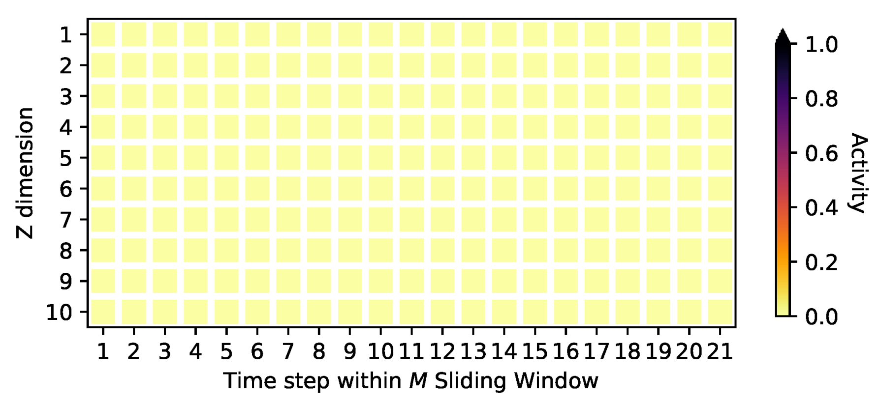
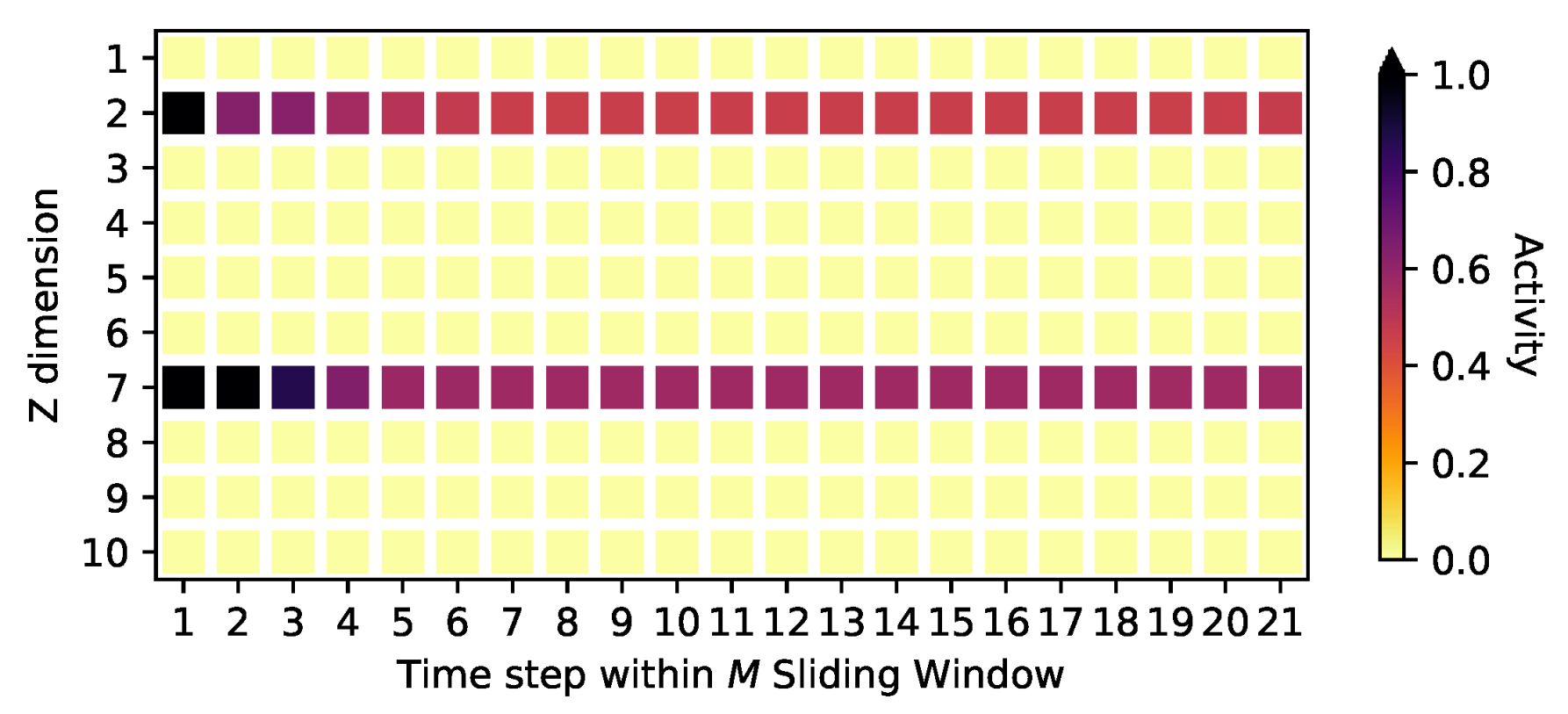
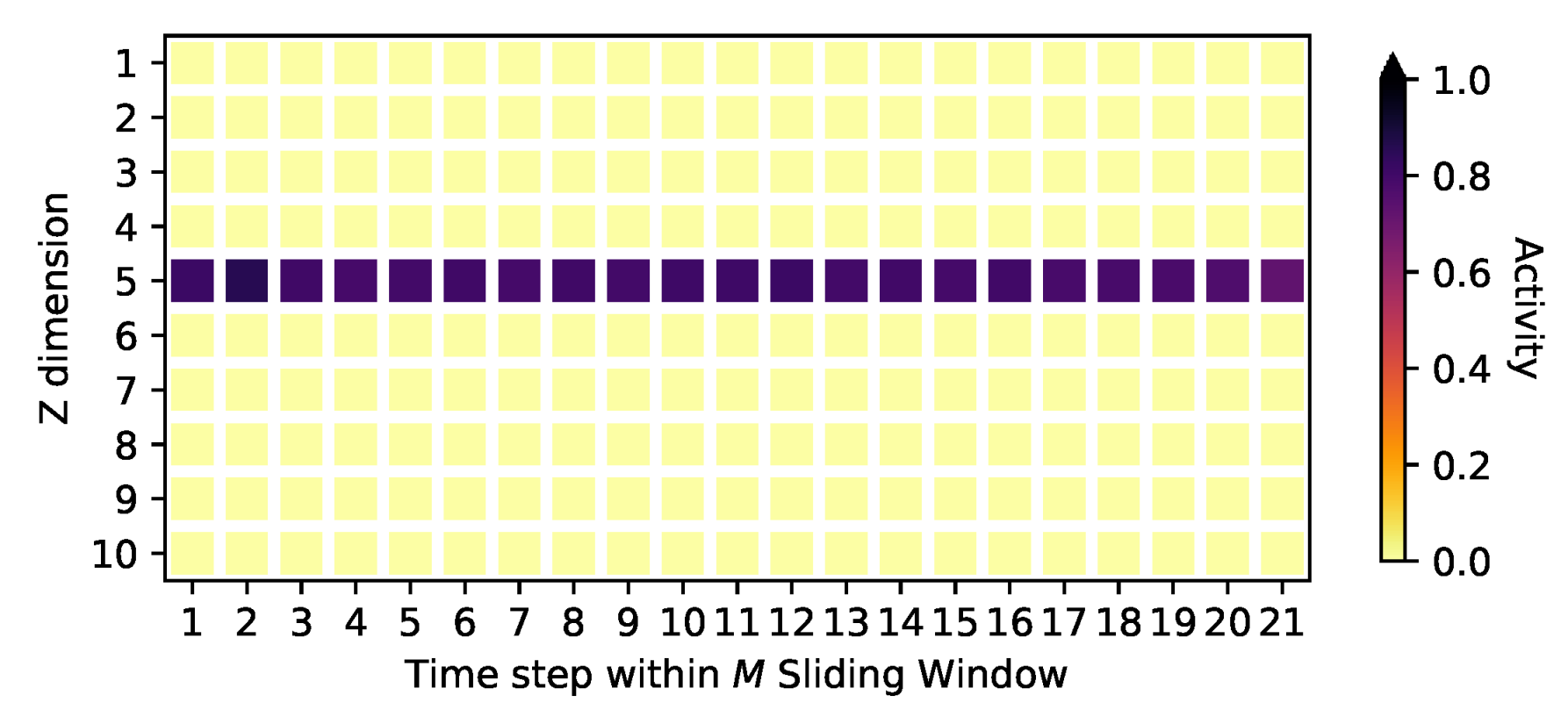
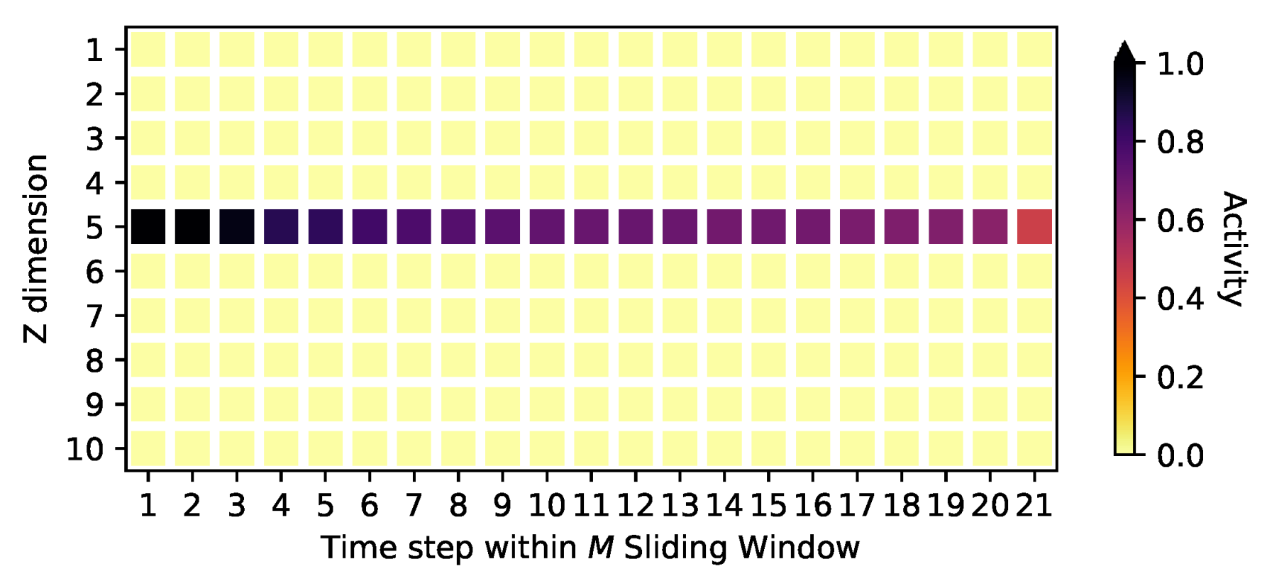
  • The signal identification analysis of the model applied to financial time series where we in particular show that the TempVAE possesses the auto-pruning property;
  • A test procedure to demonstrate that the TempVAE identifies the correct number of latent factors to adequately model the data;
  • The demonstration that our newly developed TempVAE approach for the VaR estimation performs excellently and beats the benchmark models; and
  • The detailed documentation of the hyperparameter choice in the appendix (the ablation study).
The remaining parts of our contribution are structured as follows. In Section 2, we present related work and compare it to our research. The definition of the TempVAE can be found in Section 3. In Section 4, we explain the data and provide our results for the VaR estimation with the TempVAE. We state our conclusions in Section 5. The appendix contains a detailed description of various analyses that lead to the actual form of the TempVAE that we have suggested.

2. Comparison to Related Work

VAEs are popular generative probabilistic models that allow us to model complex distributions. The models approximate a usually untractable posterior distibution by one that is easier to handle. Girin et al. (2020) provide an overview on VAEs and focus especially on dynamic VAEs. Stochastic units in RNNs, such as in dynamic VAEs, have been considered by various authors. Bayer and Osendorfer (2014), Chung et al. (2015) and Fraccaro et al. (2016) propose stochastic RNN with autoregressive structures for the observations, while Goyal et al. (2017) and Luo et al. (2018) extend the approach of (Chung et al. 2015) via auxiliary cost terms in the objective or to bidirectional RNNs, respectively. Moreover, Xu and Chen (2021) propose a similar model to (Luo et al. 2018) and apply it to financial return data.
Krishnan et al. (2017) consider a Gaussian state space model by assuming the Markov property for the latent variables and excluding autoregressive structures. Given their assumptions, they show that the true posterior for the latent variables given the observations only depends on future observations. Additionally, Fraccaro et al. (2017) consider a combination of VAE with a state space model. In particular, they assume that the observations of the state space model make up the bottleneck of the VAE. This way, they achieve a disentanglement of the latent representation and the dynamics.
Finally, Bowman et al. (2015) consider the encoding and decoding of single-layer RNN sequences via VAEs to model speech data. They argue that annealing of the regularization term is needed for learning meaningful information passing through the bottleneck.
Alternatively to the models by (Chung et al. 2015) and (Luo et al. 2018), we model a temporal dependency only in the prior distribution. Therefore, our model is similar to the deep Markov model by (Krishnan et al. 2017), but we do not use the Markov assumption.
By excluding the dependency from past realizations (the autoregressive part) for the observable returns R, the return distribution is independent from past returns but not from the past latent variables Z. Therefore, we force the encoder of the implemented model to encode as much information as possible in the latent variables Z. As a consequence, properties of conventional VAE such as the auto-pruning can be observed properly. This is not necessarily the case if we model the decoder distribution to be autoregressive on the returns R2, as assumed by (Luo et al. 2018) and (Chung et al. 2015). In this case, a substantial part of the information that can be used by the decoder would not have to pass the bottleneck. Even if the posterior q ( Z | R ) collapses and becomes independent of the input, the decoder would be able to use past observed R to achieve a good fit.
Various authors have proposed to estimate the VaR of a portfolio with artificial neural networks (ANN). Liu (2005) uses the estimates of historical simulation and GARCH as input for ANNs. Therefore, his model can be interpreted as an ensemble model. Chen et al. (2009) and Arimond et al. (2020) estimate the VaR by modeling parameters of their respective distribution assumption. Chen et al. (2009) use a standard ANN whereas Arimond et al. (2020) compare ANNs with temporal convolutional neural nets and RNNs. Arian et al. (2020) use standard VAE for the task of estimating the VaR. To account for the time dependency in the data, they preprocess the data with rolling window statistics. Fatouros et al. (2022) estimate the VaR of the underlying univariate time series composing the portfolio via a recurrent neural net. They combine the univariate VaR estimates via an estimate of the covariance matrix of the log-returns of the elements of the portfolio.
In contrast to this, in our work, we model the data not univariately but in a multivariate way. In particular, we do not have to rely on a conventionally estimated covariance matrix or on a parameterized model for the log-returns. Our approach is based on the observation that the joint log-returns of asset prices can often be projected to a lower dimensional space. By using the TempVAE for modeling the portfolio return, we can generate many realizations of the actual return (we use 1000 realizations) and then use the resulting empirical quantile of the loss function for the estimation of the VaR. Thus, the TempVAE yieds a time-dependent and, due to the auto-pruning property, parsimonious model for the data sequences.

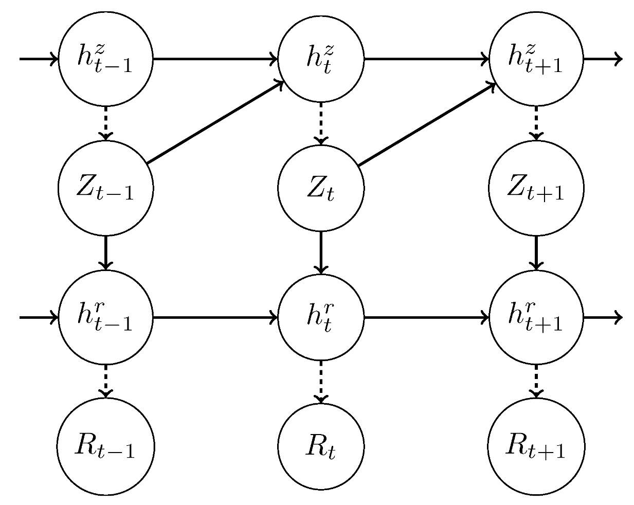
3. The Temporal Variational Autoencoder

We use the TempVAE to learn the multivariate distribution of asset returns. Therefore, we assume that the return series R = R 1 : T is generated via latent variables Z = Z 1 : T , where T N and T > 1 . The distributions of the variables Z t are estimated via approximate inference, and we expect these to hold information such as the current market environment, peer group behavior or interactions. Without further assumptions, the identification of the underlying information within the variables is usually infeasible. For example a mere rotation results in a model with the same expressiveness. Nonetheless, as we will see, the auto-pruning forces the TempVAE to model the data by only active dimensions of the latent space.
Given the two discrete-time stochastic processes R and Z, we assume an autoregressive time dependency on the latent variables given by
Z t | Z 1 : t 1 N μ z ( Z 1 : t 1 ) , Σ z ( Z 1 : t 1 ) ,
R t | Z 1 : t N μ r ( Z 1 : t ) , Σ r ( Z 1 : t ) .
Here, μ z , μ r , Σ z and Σ r are functions mapping to R κ , R d , R κ × κ and R d × d , respectively. The variables R 1 , , R T are assumed to be i.i.d. Given this dependency structure, the joint distribution can be factorized as
p θ ( Z ) = t = 1 T p θ ( Z t | Z 1 : t 1 ) ,
p θ ( R | Z ) = t = 1 T p θ ( R t | Z 1 : t ) .
To account for the dependency of the past sequences, we use RNN layers. Furthermore, we use Multi-Layer Perceptrons (MLPs) to map from the output of the RNNs to the parameter space of the distributions. In total, we use the model architecture given by
μ t z , Σ t z = MLP G z h t z ,
h t z = RNN G z h t 1 z , Z t 1 ,
Z t N μ t z , Σ t z ,
μ t r , Σ t r = MLP G r h t r ,
h t r = RNN G r h t 1 r , Z t ,
R t N μ t r , Σ t r ,
which is also depicted in Figure 1. Here, Equations (5), (6), (8) and (9) mean that the parameters on their left sides are the output of the neural networks on the right ones. These parameters then characterize the normal distributions in relations (7) and (10). h t z and h t r are defined as the hidden states of the RNNs, propagating past information through later time points. The initial states are set to zero. Combining the hidden states of the model is possible and yields a more general model formulation. However, during our experiments, it turned out to be favorable to use not trainable priors (see Appendix B.2). In order to achieve this, we separate the hidden states as shown in Figure 1.
We approximate the intractable p θ ( Z | R ) by the inference distribution q ϕ ( Z | R ) . Similar to (Krishnan et al. 2017), one can show that Z t R 1 : t 1 | Z 1 : t 1 . Therefore, we can factorize the distribution such that the variable Z t depends on the (future) observations R t : T :
p θ ( Z | R ) = t = 1 T p θ ( Z t | Z 1 : t 1 , R t : T ) .
Krishnan et al. (2017) argue that q should be factorized the same way. As q is only an approximation to p, we also considered providing the full sequence R 1 : T instead of R t : T which yields a better performance (see Appendix B.7). We therefore factorize q as
q ϕ ( Z | R ) = t = 1 T q ϕ ( Z t | Z 1 : t 1 , R 1 : T )
and assume q ϕ ( Z t | Z 1 : t 1 , R 1 : T ) N μ ^ z ( Z 1 : t 1 , R 1 : T ) , Σ ^ z ( Z 1 : t 1 , R 1 : T ) . μ ^ z and Σ ^ z are functions mapping to R κ and R κ × κ , respectively. To use the full sequence of returns R 1 : T , we implement the inference distribution via a bidirectional RNN as follows
μ ^ t z , Σ ^ t z = MLP I z h ^ t z
h ^ t z = RNN I z h ^ t 1 z , Z t 1 , h ^ t , h ^ t
h ^ t = RNN I z h ^ t 1 , R t 1
h ^ t = RNN I z h ^ t + 1 , R t + 1
Z t N μ ^ t z , Σ ^ t z .
As we have a distribution assumption with an intractable p ( Z | X ) , we train the model using the evidence lower bound (ELBO; see (Bishop 2006) Section 9.4 for a formal derivation) given as
L ( θ , ϕ ) = E q ϕ ( Z | R ) log p θ ( R | Z ) + E q ϕ ( Z | R ) log p θ ( Z ) q ϕ ( Z | R )
= E q ϕ ( Z | R ) log p θ ( R | Z ) D K L q ϕ ( Z | R ) | | p θ ( Z ) .
The components are given by Equations (3), (4) and (12). As we have log p θ ( R ) L ( θ , ϕ ) , maximization of the ELBO most likely leads to an increase in the likelihood of our distribution model. In a similar way to (Krishnan et al. 2017), we can rewrite the ELBO as
L ( θ , ϕ ) = E q ϕ ( Z | R ) log p θ ( R | Z ) t = 1 T E q ϕ ( Z 1 : t 1 | R ) [ D K L q ϕ ( Z t | Z 1 : t 1 , R ) p θ ( Z t | Z 1 : t 1 ) .
Since we assume a Gaussian distribution for q and p, we can analytically calculate the Kullback–Leibler divergence (KL-Divergence) inside the expectation in (20).

The Auto-Pruning Property of VAEs and the Posterior Collapse

The auto-pruning property of VAE originates from the KL-Divergence and has been analyzed by various authors (see Burda et al. 2016; Sicks et al. 2021). When nodes in the bottleneck are “pruned away”, it means that these nodes are not used in the neural net and therefore also not for the reconstruction. The auto-pruning capabilities of VAE are desirable, as the model focuses on useful latent representations. However, it is considered a problem when too many units become inactive before the actual learning of such a useful representation has performed some successful first steps. In the extreme case, the KL-Divergence between q ϕ ( Z | R ) and p θ ( Z ) is 0, and we have q ϕ ( Z | R ) p θ ( Z ) . Hence, q is independent of R, and we say that the posterior q collapses as the input does not matter.
As we consider multivariate Gaussian distributions with a diagonal covariance matrix, it becomes apparent that only a subset of nodes can be inactive. The posterior does not collapse in this case, as information can still be propagated to the decoder through active nodes. A diagonal covariance matrix implies independence of the latent variables Z. In order for a univariate part to be inactive, it has to be independent of the other dimensions. Nonetheless, the overall independence is not a necessity to monitor inactivity. For example, block-wise covariance matrices would result in batches of active or inactive latents.
When using the TempVAE on financial data, we observe an instantaneous collapse of the posterior at the beginning of the training. From our point of view, the signal within the financial returns data is not strong enough to be captured before the KL-Divergence term dominates the ELBO and causes a posterior collapse. Therefore, we consider β -annealing of the KL-Divergence similar to (Bowman et al. 2015) (see Appendix A).
To measure the amount of active units, Burda et al. (2016) propose an activity statistic that is calculated after training. For each node, they estimate the activity by
A u = Cov x E q ϕ u | x [ u ]
and call a node inactive if A u < 0.01 . The intuition behind this statistic is as follows. If for given inputs x, the expected values in a latent dimension do not show significant variability, the resulting latent dimension has no useful information of the input and is seen as independent.
Since we assume a time-dependent model for the prior in (3), we adjust the activity statistic to calculate the activities of a sequence of Z 1 : M R M × κ . For m = 1 , , M and k = 1 , , κ , we calculate
A z ( m , k ) : = Cov R , Z 1 : m 1 E q ϕ Z m , k | Z 1 : m 1 , R Z m , k E p θ Z m , k | Z 1 : m 1 Z m , k .
The statistic becomes equal to the one proposed by (Burda et al. 2016) if we assume a time-independent standard Gaussian prior3 in (3). With the statistic in (21), we quantify the effect of the input R. Similar to (Burda et al. 2016), we call a node inactive from the input if A z ( m , k ) < 0.01 .

4. Implementation, Experiments and VaR-Estimation

In this section, we present the results we achieved on four datasets (see Section 4.1) with our model regarding the identification of the underlying signal (see Section 4.2). Then, in Section 4.3, we present results for the fit to financial data as well as the VaR estimation. For further details on the model implementation and for an additional ablation study validating our design choices, see Appendix A and Appendix B.

4.1. Description of the Used Data Sets

We consider the four datasets “DAX”, “S&P500”, “Noise” and “Oscillating PCA” for our studies. Here, the last two datasets are simple artificial examples with the only purpose to check the correct performance of the TempVAE. Throughout the section, data are stored in d-dimensional vectors
R t : = R t , 1 , , R t , d T R d .
First, we consider (d = 22) stock price time series, provided by DAX (German stock index) enlisted companies, from 11.06.2001 to 09.06.2021. We calculate the daily logarithmic returns4 via the observed closing prices. Therefore, if S t , i denotes the price of stock i = 1 , , d at time t = 1 , , T , the dataset “DAX” contains
R t , i : = ln S t , i ln S t 1 , i .
For “S&P500”, we consider 397 stocks of the S&P500 index that have a history from 02.01.2002 up to 09.06.2021. We calculate the log-returns analogously to the “DAX” data.
The dataset “Noise” is just white noise with dimension d = 22 . Hence, for all t = 1 , , T and i = 1 , , d
R t , i N 0 , 1 .
The dataset “Oscillating PCA k” (with k { 2 , 5 , 10 } ) is constructed based on k independent harmonic oscillator signals. Each univariate signal Z 1 : T is constructed by randomly choosing an intercept i U 1 , 1 , an amplitude a U 1 , 1 , a frequency f U 0.5 , 24 and a noise series ϵ 1 : T , with ϵ N 0 , 0.02 2 . Then, we set
Z t = i + a · cos t 100 · f · π + a · ϵ t .
The case k = 2 is shown in Figure 2. The oscillator sequences Z 1 : T , 1 : k R T × k are then transformed to a 22-dimensional series by applying a randomly chosen rotation U R d × k :
S t = U · Z t , 1 : k T + 5 and R t , i : = ln S t , i ln S t 1 , i
for each t = 1 , , T and i = 1 , , d .
Finally, a sliding window is applied to the d-dimensional series R 1 : T to generate T M consecutive series in R d × M of size M = 21 . For further details on preprocessing procedures, see Appendix A.

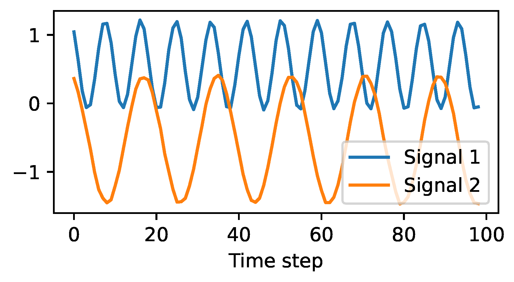
4.2. Signal Identification

We train the TempVAE on the four datasets from Section 4.1 and analyze calculated activities given by (21) as well as the fit to the data. As we can see in Figure 3 and Figure 4, the TempVAE correctly identifies the amount of hidden dimensions. For the “Noise” data, no activity is reported at all. The decoder model p ( R | Z ) is left on its own to model the data as no meaningful information can be identified that can be propagated from input to output. For the data “Oscillating PCA 2”, the model correctly identifies the two active nodes per timestep. For the “Oscillating PCA 5” and “Oscillating PCA 10” data, the model also identifies two active dimensions through time (see Appendix D). Although this is not the amount given by the linear construction, identifying fewer dimensions is not necessarily problematic, since we have a non-linear model. We observe comparable fitting results for these datasets (see Appendix D).
When applied to the financial data, we can observe two and four active dimensions for the “DAX” and “S&P500” datasets, respectively (see Appendix E). The fact that only a few active nodes could be identified is not surprising. In their work, Laloux et al. (2000) show that only a small fraction of dimensions (roughly 11) are needed to linearly model 406 assets of the S&P500 during the years 1991–1996.

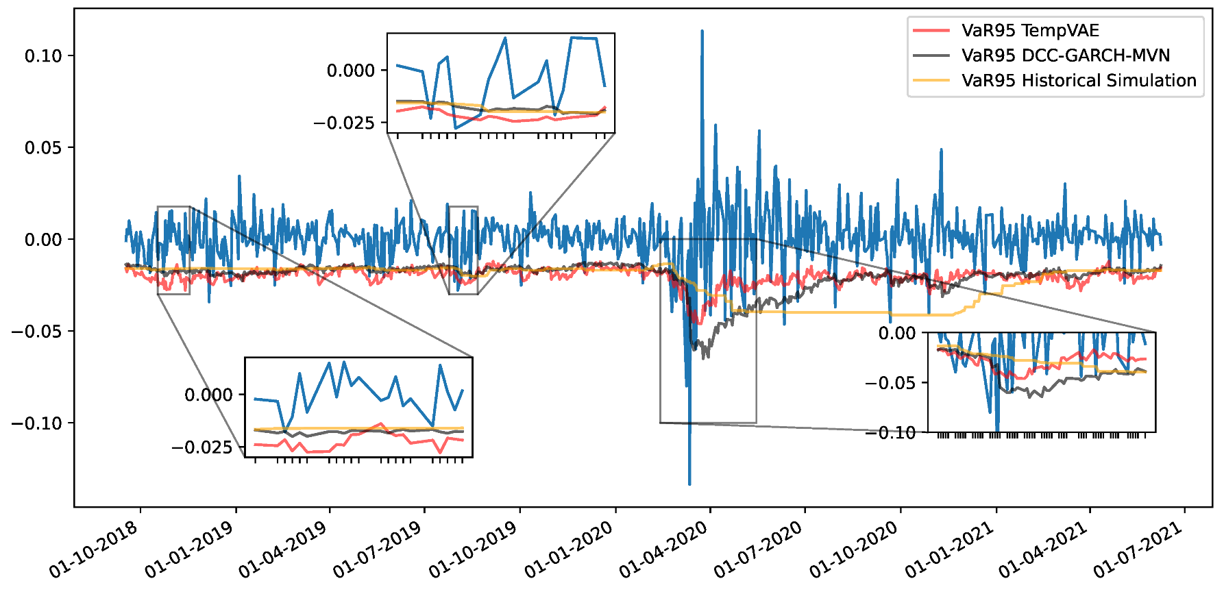
4.3. Fit to Financial Data and Application to Risk Management

To assess the performance of the model on the “DAX” data5, we compare the TempVAE to a GARCH model as well as to the multivariate GARCH versions DCC-GARCH-MVN and DCC-GARCH-MVt (see Appendix C for details). The capacities of these models are less compared to the used TempVAE neural net. Nonetheless, GARCH and its variants are market standard for VaR calculation. To underline the usefulness of a model, the results have to be compared to these benchmarks.
To compare the models, we calculate the negative log-likelihood (NLL), which is given by
NLL ( R t nonlog , μ t , Σ t ) : = 1 2 d log 2 π + log Σ t + R t nonlog μ t T Σ t 1 R t nonlog μ t
and average across all timestamps in the test set. R t nonlog represents the non-logarithmic returns of the test data and μ t as well as Σ t are estimated by the models. To estimate these values, we first sample the log-returns from a model. For the TempVAE, we estimate these empirically by sampling
z 1 : t ( i ) q ϕ ( Z | r 1 : t 1 ) as well as r t ( i ) p θ ( R | z 1 : t ( i ) )
for i = 1 , , 1000 . Then, we transform these samples to non-log-returns and calculate the empirical means and covariances to approximate μ t and Σ t .
We also consider the diagonal NLL, where we use the diagonal matrix with entries d i a g Σ t instead of Σ t . Furthermore, we calculate a univariate version by considering the returns of an equally weighted portfolio containing the 22 assets. Given the log-returns in (23), we calculate these by
R t , i P , nonlog : = 1 d i = 1 d exp R t , i 1 .
Table 1 displays the different fit scores for the three models. Considering the NLL scores, the GARCH and normal DCC-GARCH models achieve the best performance since these models are directly minimizing the respective scores. The TempVAE as a regularized model has to find a trade-off between the NLL and the regularization terms. Nonetheless, if we consider the scores for the portfolio returns, we see all multivariate models performing similarly and outperforming the GARCH model. Due to the strong dependency between the different assets in the portfolio, estimating the underlying covariance structure plays an essential role in estimating the next day’s portfolio performance. Furthermore, we could observe the models capturing the correlations between the assets (see Appendix F for an excerpt of the first two dimensions).
To compare the performance on the VaR estimation, as a further method, we consider historical simulation (HS).6 Then, for each method, we calculate the VaR estimates via 1000 Monte Carlo samples from the respective distributions.7 VaR95 then denotes the empirical estimator for the 95 % -Value-at-Risk which is the 50th value of the ordered samples of returns (arranged from lowest to highest). VaR99 denotes the corresponding estimator given as the 10th value of the ordered sample. For this, also note that we are looking at the actual returns, i.e., the negative of the losses.
We compare the models by their average number of exceedances, i.e., when the VaR estimate was higher then the observed return, within the test set. We below denote these values by AE95 and AE99, and they help us to validate the VaR estimates by their 5% and 1% quantile assumption. A good performance is a necessary condition for filtering out those candidates that we compare with respect to a further criterion.
As this second performance check, we use the ‘Regulatory Loss Function’ (RLF) proposed by (Sarma et al. 2003). This score penalizes exceedances of observed returns below the VaR and is given by
RLF VaR t , r t = VaR t R t 2 , if R t VaR t 0 , otherwise .
Here, R t denotes the value of the (non-logarithmic) portfolio return at time t. We calculate the average of these values over the test set.
In Table 2, the losses for the models as well as the average number of exceedances are displayed. The amount of average exceedances helps us to validate the VaR estimates by their 5% and 1% quantile assumption, and a good performance is a necessary condition. As the number of exceedances of a predicted VaR t does not look at the size of the exceedances8, we have introduced RLF as an additional criterion to judge among those models that are good in estimating the average number of exceedances. As small numbers of RLF show that the VaR t requires a high reserve when it is needed, a small RLF value is good. Therefore, although DCC-GARCH-MVt has the lowest values for the RLF95 and RLF99, the TempVAE produces the best estimates.
In Figure 5, the VaR95 values for the DCC-GARCH-MVN, HS and TempVAE are displayed. The blue line shows the original returns of the DAX portfolio. The full path of the VaR95 estimates as well as the VaR99 estimates can be found in Appendix F. We can see the VaR95 estimates for the DCC-GARCH-MVN and TempVAE are quickly responding to the changes in the volatility of the data. Comparing TempVAE directly to DCC-GARCH-MVN, we see the VaR estimates to be more volatile but also responsive to the evolution of the returns. The HS on the other side is showing the well-known time delay (see Liu 2005). Even though in terms of average exceedances, the HS is best followed by TempVAE, in our point of view, the TempVAE provides the most reasonable estimates among the models. This is particularly supported by the RLF values.

5. Conclusions

In this paper, we present a novel variational recurrent neural net with the well-known bottleneck structure of autoencoders to handle sequential data. As we model the data on the basis of a time-dependent prior, we call the model temporal variational autoencoder (TempVAE). By ensuring that the information has to flow through the bottleneck, we leverage the auto-pruning property of VAE. This way, we are able to find parsimonious model representations of the data without using methods such as grid search.
We successfully apply the TempVAE to risk management. More precisely, we estimate the risk measure VaR and show that our model performs competitively to the considered benchmark models. We provide a roughly unbiased estimation of VaR exceedances, showing the model is performing best in terms of the considered RLF scores.
Future research directions can incorporate applying the TempVAE architecture to other types of data sequences. Furthermore, the active dimensions in the bottleneck are not necessarily yielding disentangled representations. Research in this direction can foster the understanding of the auto-pruning and hence variational models further.

Author Contributions

Conceptualization, R.B. and R.K.; methodology, R.B. and I.R.; software R.B.; validation, R.B., S.G., R.K. and I.R.; formal analysis, R.B.; data curation, R.B.; writing—original draft preparation, R.B., S.G., R.K. and I.R.; writing — review and editing, R.B., R.K.; visualization, R.B.; All authors have read and agreed to the published version of the manuscript.

Funding

Robert Buch gratefully acknowledges the financial support via a PhD grant from the Fraunhofer ITWM.

Data Availability Statement

Both the DAX data and the S&P 500 data are publicly available.

Conflicts of Interest

The authors declare no conflict of interest.

Appendix A. β-Annealing, Model Implementation and Data Preprocessing

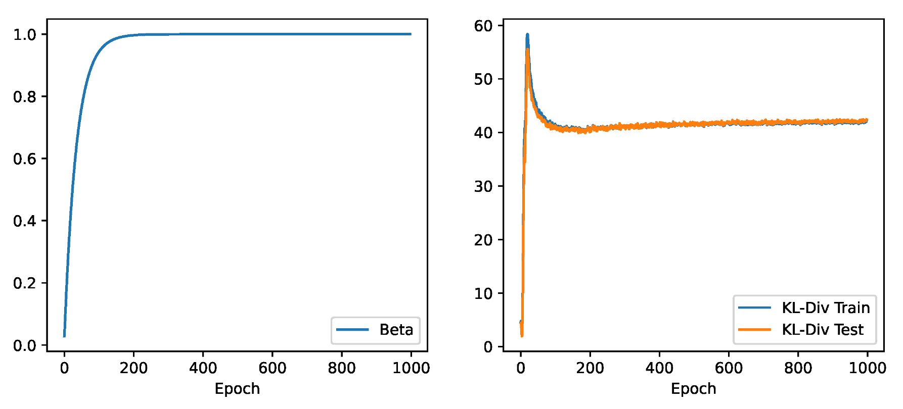
Appendix A.1. β-Annealing

The low signal-to-noise ratio in financial data makes it necessary to proceed delicately when modeling financial data. We propose to use annealing of the regularization to mitigate the initial effects of the auto-pruning. Specifically, we consider β -annealing of the KL-Divergence similar to Bowman et al. (2015). We add β 0 to the ELBO in (20) to obtain
L β ( θ , ϕ ) = E q ϕ ( Z | R ) log p θ ( R | Z ) β · t = 1 T E q ϕ ( Z 1 : t 1 | R ) [ D K L q ϕ ( Z t | Z 1 : t 1 , R ) p θ ( Z t | Z 1 : t 1 ) .
The KL influence is adjusted over β . During training, we start with β = 0 and increase it over time. In Figure A1, the annealing over 1000 epochs is depicted, and the effect on the KL-Divergence is shown as well.
Figure A1. On the left: The KL influence is adjusted over β . During training, we start with β = 0 and increase it over time. We implement this by subtracting an exponentially decaying term from the ultimate β value. We use a decay rate of 0.96 and decay steps of 20. On the right: The evolution of the (negative) KL-Divergence over time. We can see how the values starts to decrease after the annealing has increased β enough.
Risks 11 00079 g0a1

Appendix A.2. Model Implementation

We implement the model based on Section 3. For the RNNs, we choose ‘Gated Recurrent Units’ (see Cho et al. 2014) with dimension 16, and the initial values of these states are set to zero. For the MLPs, we use normal Feedforward Networks that have two hidden layers with dimension 16 and the output layer with varying output dimension. For the latent variables, we choose dimension 10. In our experiments, with this size of the latent dimension, the model is overspecified, and the auto-pruning removes the dimensions that are not needed.
We initialize all MLP layer weights with the ‘Variance Scaling’ initializer as proposed by He et al. (2015). As the activation function for the hidden layers, we use the ‘Rectified Linear Unit’ (ReLU). For the μ z , μ ^ z and μ r layer, we use no activation. We use a diagonal covariance structure for Σ z and Σ ^ z and a rank-1 perturbation output as given in Rezende et al. (2014) for Σ r . For all covariance layers, we use exponential activation for the diagonal entries. Furthermore, we add L2 regularization with parameter λ = 0.01 for the weights of the hidden layers of the MLP as well as dropout with a rate of 10 % to the RNN layers. In our experiments, both the dropout and the L2 regularization turned out to be crucial for the auto-pruning to work properly as well as for an adequate data modeling (see Appendix B.6).
In contrast to the model of Luo et al. (2018), we set the parameters of the prior (i.e., Equations (5)–(7)) as non-trainable. Allowing a trainable prior results in an unfavorable performance regarding the signal identification as well as the risk-management application (see Appendix B.2). In our point of view, the fixed prior serves as guidelines for the model to identify temporal transitions. If the prior is learned simultaneously with the encoder, past adaptions of the encoder to the temporal dynamics can become obsolete by changes in the prior parametrization.
For the training of the model, we use the reparametrization trick as introduced by Kingma and Welling (2014). Using the ADAM optimizer by Kingma and Ba (2015), we train the model for 1000 epochs with a batch size of 256. We use an initial learning rate of 0.001 with an exponential learning rate decay with a decay rate of 0.96 and 500 decay steps. If not explicitly excluded, we apply the β -annealing as described in Figure A1 during training.

Appendix A.3. Data Preprocessing

To model the data with artificial neural networks, we split the data into a training and test set. Furthermore, we use the empirical mean and standard deviation of the training part to standardize each ( i = 1 , , d ) univariate series R 1 : T , i . Finally, we apply a sliding window on the d-dimensional series in (22) to generate T M intervals of size M = 21 . We define
R t : t + M : = R t , , R t + M R d × M ,
for t = 1 , , T M . After the preprocessing, we have different amounts of observations which we split into 66% training and the rest into test data:
  • For the DAX data, 5061 observations were split at t = 3340 into 3340 training observations and 1721 test observations.
  • For the S&P500 data, 4872 observations were split at t = 3215 into 3215 training observations and 1657 test observations.
  • For the noise data, 5050 observations were split at t = 3333 into 3333 training observations and 1717 test observations.
  • For each of the oscillating PCA datasets, 9979 observations were split at t = 6586 into 6586 training observations and 3393 test observations.

Appendix B. Ablation Studies

In this section, we validate some of the design choices for the TempVAE model. We will address each point in a separate section, starting off with the β -annealing.

Appendix B.1. Preventing Posterior Collapse with β-Annealing

A deep neural net such as the TempVAE has to be trained with caution to prevent posterior collapse. The β -annealing proposed in Appendix A is a useful tool to prevent this collapse. In this section, we compare the TempVAE with a model ‘TempVAE noAnneal’ with no annealing, where we set β = 1 instead of using β -annealing. Given the activity statistics of a model A z ( m , k ) , as described in (21) for m = 1 , , M and k = 1 , , κ , we calculate the average number of active units as
A ¯ z : = 1 M · κ m = 1 M k = 1 κ 𝟙 A z ( m , k ) 0.02
In Table A1, we see the average number of active units for the two models and in Table A2, the NLL scores as calculated in Section 4.3 are reported.
Table A1. The average number of active units given by (A2) for the two models with and without annealing. We see that the model with the annealing is not decreasing the number of average active dimensions when increasing the number of latent signals. For the model without annealing, this is not the case.
DAXNoiseOsc. PCA 2Osc. PCA 5Osc. PCA 10
TempVAE20%0%20%20%20%
TempVAE noAnneal0%0%10%20%10%
Table A2. The negative log-likelihood for the two models on the test set. We see the TempVAE is outperforming the version without annealing on every relevant dataset. Only for the noise case, where there is nothing to learn, are the results comparable.
DAXNoiseOsc. PCA 2Osc. PCA 5Osc. PCA 10
TempVAE20.2931.48−38.51−1.4011.07
TempVAE noAnneal27.4931.443.582.6013.28
Using the annealing, a latent process in financial data is identified. Without annealing, a posterior collapse occurs and no encoding information is propagated to the decoder. Notice that the amount of active dimensions need not match the amount of latent signals. Because of non-linearities, it can be possible for the model to use less dimensions than needed to adequately model the data (see Appendix D).

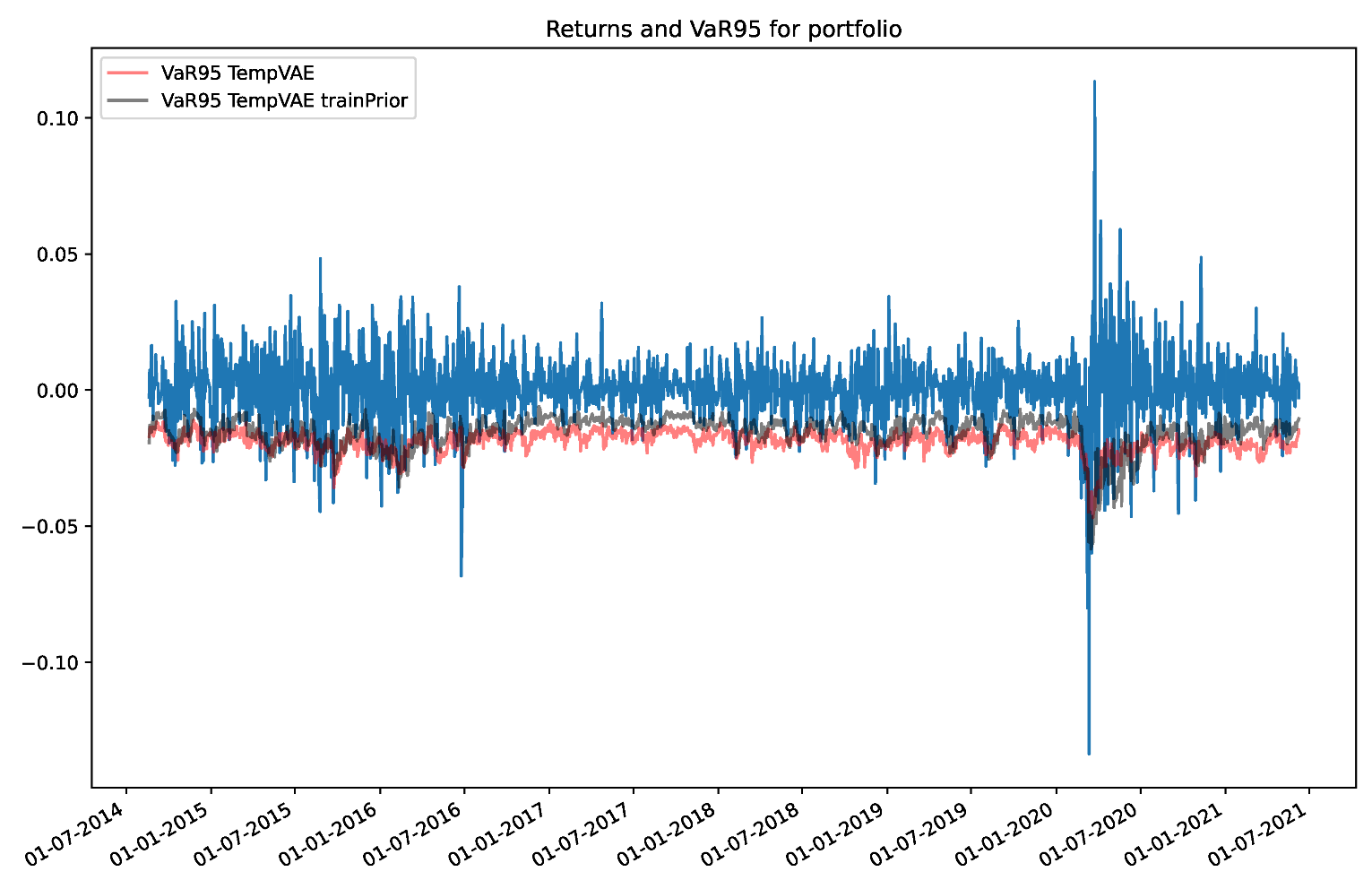
Appendix B.2. Comparison to a Model with Trainable Prior Parameters

In this section, we find that using a non-trainable prior p θ ( Z ) yields better results in terms of the auto-pruning functionality as well as of the fit of the model. To see this, we compare the TempVAE model with a version ‘TempVAE trainPrior’, where the prior is trainable. Figure A2 and Figure A3 display the activities of the ‘TempVAE trainPrior’ bottleneck for the DAX data and for the oscillating PCA data, respectively.
Figure A2. The activity statistics for the “DAX” data for the model ‘TempVAE trainPrior’. We consider sequences of size M = 21 as input. The graph shows the activity values of statistic (21) for the κ = 10 dimensional latent space.
Risks 11 00079 g0a2
Figure A3. The activity statistics for the “oscillating PCA” data for the model ‘TempVAE trainPrior’. We consider sequences of size M = 21 as input. The graph shows the activity values of statistic (21) for the κ = 10 dimensional latent space.
Risks 11 00079 g0a3
Comparing these figures with Figure 4, we notice that the value of the activity statistics drastically decreased. For the model with trainable prior, it is questionable if any information from the input is propagated to the output for the ‘Oscillating PCA’ data at later time steps.
Comparing the VaR forecasts of both models in Figure A4, we see that the VaR forecasts for the model with trainable prior are more volatile. This also affects the average amount of exceedances of this estimator, as can be seen in Table A3. The TempVAE outperforms the version with trainable prior, as the amount of exceedances for the VaR95 should be close to 5, and for VaR99, they should be close to 1. From our point of view, setting the prior as non-trainable gives the model more stability during training. This results in a more consistent output, e.g., for the VaR estimates.
Table A3. The average exceedances for the model TempVAE and the version with trainable parameters for the prior p θ ( Z ) . TempVAE outperforms the trainable prior version. For the average exceedances, the respective quantile assumption is the optimal value. Hence, for VaR95, the best value is 5, and for VaR99, the best value is 1.
ModelAE95AE99
TempVAE4.81.3
TempVAE trainPrior8.23.1
Figure A4. VaR95 forecasts of both models ‘TempVAE’ and ‘TempVAE trainPrior’ on the test set. The VaR forecasts for the model with trainable prior are more volatile.
Risks 11 00079 g0a4

Appendix B.3. Autoregressive Structure for the Observables Distribution

Modeling an autoregressive connection for the observations produces questionable results due to over-fitting. In this section, we compare the model TempVAE with the model ‘TempVAE AR’, a version of the model with autoregressive structures as proposed, e.g., by Chen et al. (2023) or Luo et al. (2018). The implementation of the model ‘TempVAE AR’ is identical to the model TempVAE except for the generative distribution. Instead of (8)–(10), we implement this part as
μ t r , Σ t r = MLP G r h t r ,
h t r = RNN G r h t 1 r , z t , r t 1 ,
r t N μ t r , Σ t r .
Therefore, past observations are influencing the current distributions. If such a dependency structure is assumed given a sequence of observations R 1 : T , the latent variables become dependent on the whole observed sequence, as argued in Luo et al. (2018). As we account for this already in our proposed model for the encoder (see (13)–(17)), we do not have to adapt for this part.
Looking at Table A4, we see that TempVAE outperforms ‘TempVAE AR’ on all test sets. In fact, we can observe over-fitting for the ‘TempVAE AR’ model, whereas the TempVAE did not suffer from this. Common VAEs possess an inherent robustness against over-fitting (see e.g., Kingma et al. 2014) originating from the regularization with the KL-Divergence. As the structure of the TempVAE enforces this regularized bottleneck structure, we are not surprised that we do not observe over-fitting with the TempVAE. On the other side, ‘TempVAE AR’ has the possibility to ignore the regularized bottleneck, and hence, over-fitting becomes more of a concern.
Table A4. The negative log-likelihood for the two models TempVAE and ‘TempVAE AR’ on the test set. We see that the TempVAE is outperforming the version with an autoregressive structure, even in the case of the Noise dataset. This is because the ‘TempVAE AR’ model was over-fitting these data.
DAXNoiseOsc. PCA 2Osc. PCA 5Osc. PCA 10
TempVAE20.2931.48−38.51−1.4011.07
TempVAE AR22.6832.91−34.7225.3369.26
Apart from these results, another point speaks in favor of the TempVAE without an autoregressive structure for the observations. As information does not necessarily have to pass the bottleneck, analyzing the latent space activity becomes tedious. Even for a completely collapsed posterior q, the model can use information from the input sequence to model the output.

Appendix B.4. Using a Diagonal Covariance Matrix Σ t r

Here, we compare the ‘TempVAE’ with the model ‘TempVAE diag’, a version of the model, where the output covariance matrix for the observables is modeled as diagonal and not via the rank-1-perturbation as given in Appendix A. As we can see in Table A5, the average amount of VaR exceedances is approximately the same for the two model architectures. This indicates that by the usage of the latent variables, the covariance structure of the data can be explained well enough to obtain a comparable performance for the VaR estimates. We still decided to propose the rank-1 perturbation for the model, as Luo et al. (2018) were able to improve their fit this way.
Table A5. The average exceedances for the model TempVAE and the version with diagonal covariance matrix for Σ t r . For the average exceedances, the respective quantile assumption is the optimal value. Hence, for VaR95, the best value is 5, and for VaR99, the best value is 1.
ModelAE95AE99
TempVAE4.81.3
TempVAE diag5.31.6

Appendix B.5. Setting μ t r 0

In their paper, Xu and Chen (2021) motivate to model only the covariance Σ t r of the observable distribution (2). We therefore compare the TempVAE with the model ‘TempVAE zeroMean’, which is the same model but with the mean parameter fixed to an output of zero. Figure A5 and Figure A6 show the activity statistics for the “DAX” and “Oscillating PCA 2” datasets.
Figure A5. The activity statistics for the “DAX” data for the model ‘TempVAE zeroMean’. We consider sequences of size M = 21 as input. The graph shows the activity values of statistic (21) for the κ = 10 dimensional latent space.
Risks 11 00079 g0a5
Figure A6. The activity statistics for the “Oscillating PCA 2” data for the model ‘TempVAE zeroMean’. We consider sequences of size M = 21 as input. The graph shows the activity values of statistic (21) for the κ = 10 dimensional latent space.
Risks 11 00079 g0a6
Here, we can observe that the number of identified active nodes per timestep is less in comparison with the TempVAE model. A smaller latent space occupation than given by the amount of latent signals is possible due to the non-linearities of the net. However, from our point of view, it is rather questionable that one latent dimension suffices to capture the signal in both the “Oscillating PCA 2” dataset and the “DAX” dataset. Furthermore, comparing the kernel density estimated distributions of the “Oscillating PCA 2” dataset in Figure A7 and Figure A12, we see that the model is not able to correctly model the two dimensions of the signal inherent in the data. Therefore, we decide to model the mean parameter.
Figure A7. The kernel density estimated distribution of the “oscillating PCA 2” data. On the left, we see the model ‘TempVAE zeroMean’ and on the right, the historical data.
Risks 11 00079 g0a7

Appendix B.6. Regularization: L2, Dropout and KL-Divergence

In this section, we compare the TempVAE to five other models where different regularization procedures are set as inactive. The models we consider are
  • ‘TempVAE’.
  • ‘TempVAE det’: The KL-Divergence is switched off and the bottleneck uses only a mean parameter whereas the covariance is set to zero. Therefore, the bottleneck is deterministic and the auto-pruning switched off.
  • ‘TempVAE no dropout/L2’: Dropout and L2 regularization are switched off.
  • ‘TempVAE no L2’: L2 regularization is switched off.
  • ‘TempVAE no dropout’: Dropout is switched off.
  • ‘TempVAE det no dropout/L2’: ‘TempVAE det’ and ‘TempVAE no dropout/L2’ combined.
In Table A6, the average number of active dimensions is shown. As we can see, only the model ‘TempVAE’ is providing favorable results. The deterministic models show no auto-pruning for the Oscillating PCA data versions while the model ‘TempVAE det no dropout/L2’ is even activating most of the latent nodes when modeling the Noise data. This extensive use of bottleneck nodes is a sign of over-fitting. It is important to understand that if the KL-Divergence is switched off for these models, the reconstruction error, that is, the first term in Equation (A1), is the only factor driving the encoder model training. Hence, the encoder aims to provide latent variables that are best suited for reconstruction just as in a normal autoencoder model. Since the encoder and prior distribution are disconnected without the KL-Divergence term, the forecast of these models is highly doubtful. Nonetheless, the reconstruction has been learned, and therefore, we can analyze the latent space activity.
The stochastic models without L2, dropout or both also show questionable results. Therefore, we conclude that both regularizations are essential to learn the deep neural net and for the auto-pruning to work properly.
Table A6. The average number of active units given by (A2) for the models where different regularizations are excluded.
DAXNoiseOsc. PCA 2Osc. PCA 5Osc. PCA 10
TempVAE20%0%20%20%20%
TempVAE det0%0%90%81%90%
TempVAE no dropout/L220%0%31%76%30%
TempVAE no L220%6%20%20%30%
TempVAE no dropout20%0%31%41%40%
TempVAE det no dropout/L290%90%90%80%90%
Furthermore, we found that none of the models without dropout were able to adequately model the data structure of the “Oscillating PCA 2”. Figure A8 displays the kernel density estimated distribution of the first two dimensions of the data “Oscillating PCA 2”. In contrast to Figure A12, the plot for the model ‘TempVAE’ structure is poorly fit.
Figure A8. The kernel density estimated distribution of the “oscillating PCA 2” data for the model ‘TempVAE no dropout’. On the left, we see the ‘TempVAE no dropout’ model and on the right, we see the historical data.
Risks 11 00079 g0a8

Appendix B.7. Encoder Dependency

In this section, we compare the ‘TempVAE’ model with ‘TempVAE backwards’, which is a version where the encoder structure is not implemented as in (13)–(17), but with a backward RNN, which is given by
μ ^ t z , Σ ^ t z = M L P I z h ^ t z
h ^ t z = R N N I z h ^ t 1 z , z t 1 , h ^ t
h ^ t = R N N I z h ^ t + 1 , r t + 1
z t N μ ^ t z , Σ ^ t z .
This is in consensus with the dependency structure of the posterior p θ ( Z | R ) , which is shown in (11).
Figure A9 displays the KDE estimation of the first two dimensions of the oscillating PCA data. In contrast to Figure A12, the plot for the model ‘TempVAE’ structure is poorly fit.
Figure A9. The kernel density estimated distribution of the “oscillating PCA 2” data for the model ‘TempVAE backwards’. On the left, we see the ‘TempVAE backwards’ model and on the right, we see the historical data.
Risks 11 00079 g0a9
Table A7 shows that the auto-pruning is performing poorly when using only the backwards RNN for the model. As the encoding model is only a variational approximation to the actual posterior, we therefore decide to use the bidirectional architecture for our model.
Table A7. The average number of active units given by (A2) for the two models with different encoder architecture.
DAXNoiseOsc. PCA 2Osc. PCA 5Osc. PCA 10
TempVAE20%0%20%20%20%
TempVAE backwards10%0%10%0%0%

Appendix C. GARCH and DCC-GARCH

As benchmarks for the fit of the financial data, we consider three models.
  • GARCH: A GARCH(1,1) model, introduced by Bollerslev (1986).
  • DCC-GARCH-MVN: A Dynamic Conditional Correlation GARCH(1,1), introduced by Engle (2012), with a multivariate Gaussian distribution assumption for the error term.
  • DCC-GARCH-MVt: A Dynamic Conditional Correlation GARCH(1,1), with a multivariate distribution assumption for the error term.
As the GARCH model is univariate, we model each dimension of our observed data separately. Therefore, we assume a correlation of 0 among the observed assets. The DCC-GARCH models can be seen a a multivariate extension of the first, where the correlations are modeled as well. All models are linear and optimized by using the Maximum Likelihood principle. We used the ‘rmgarch’ library in R (see Ghalanos 2019).

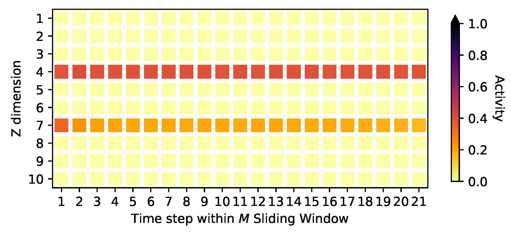
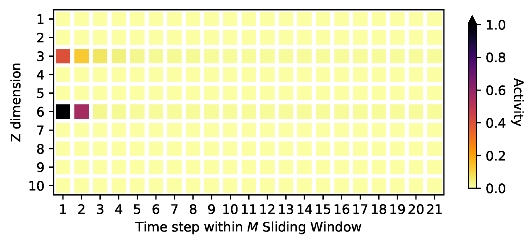
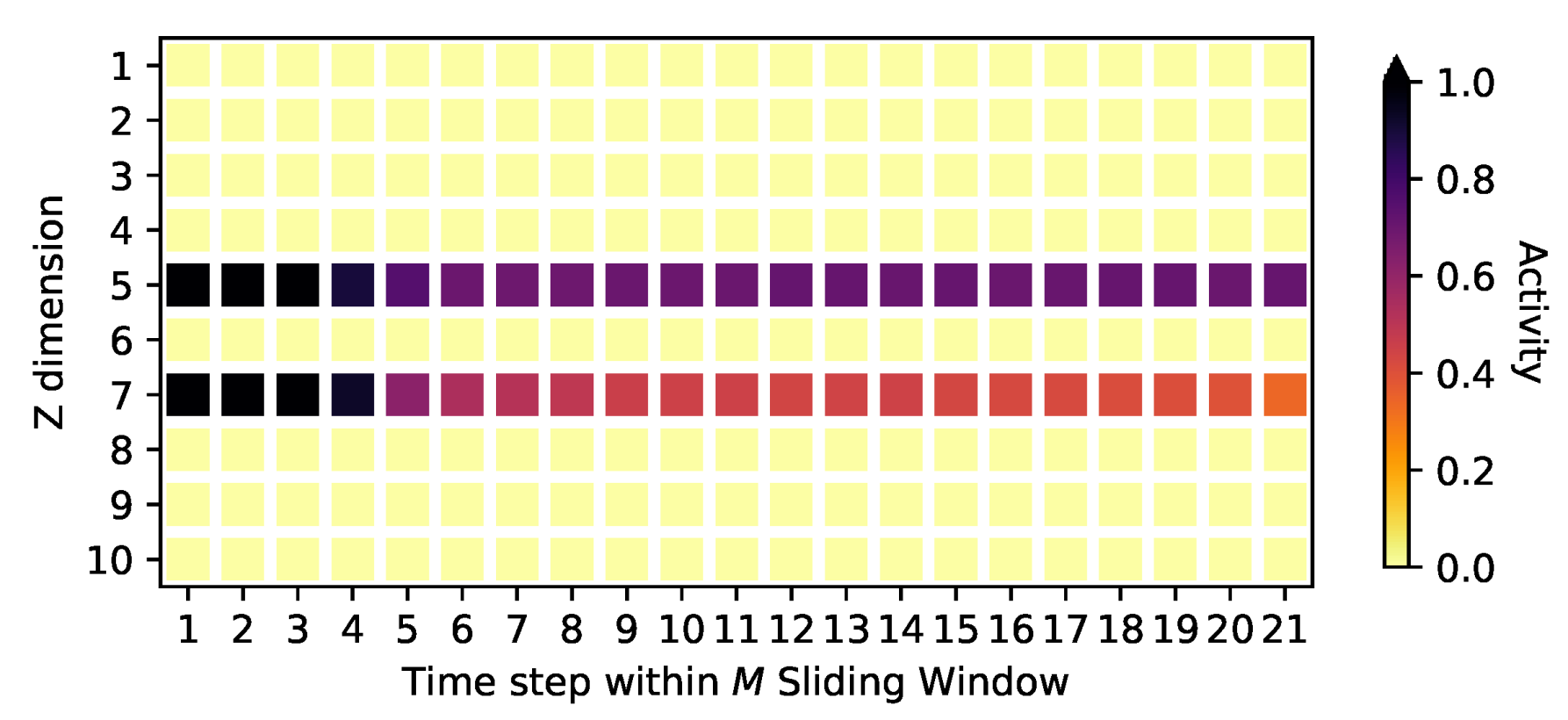
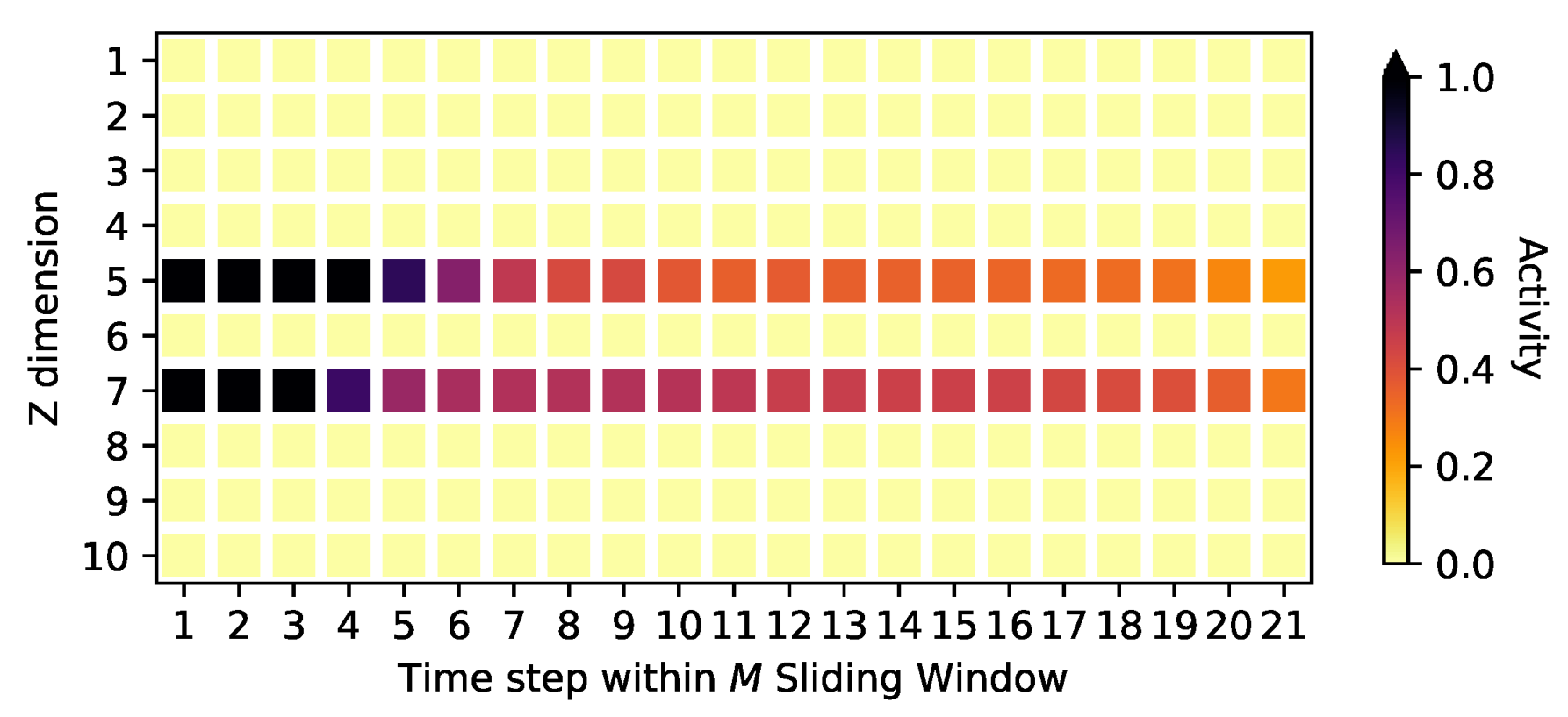
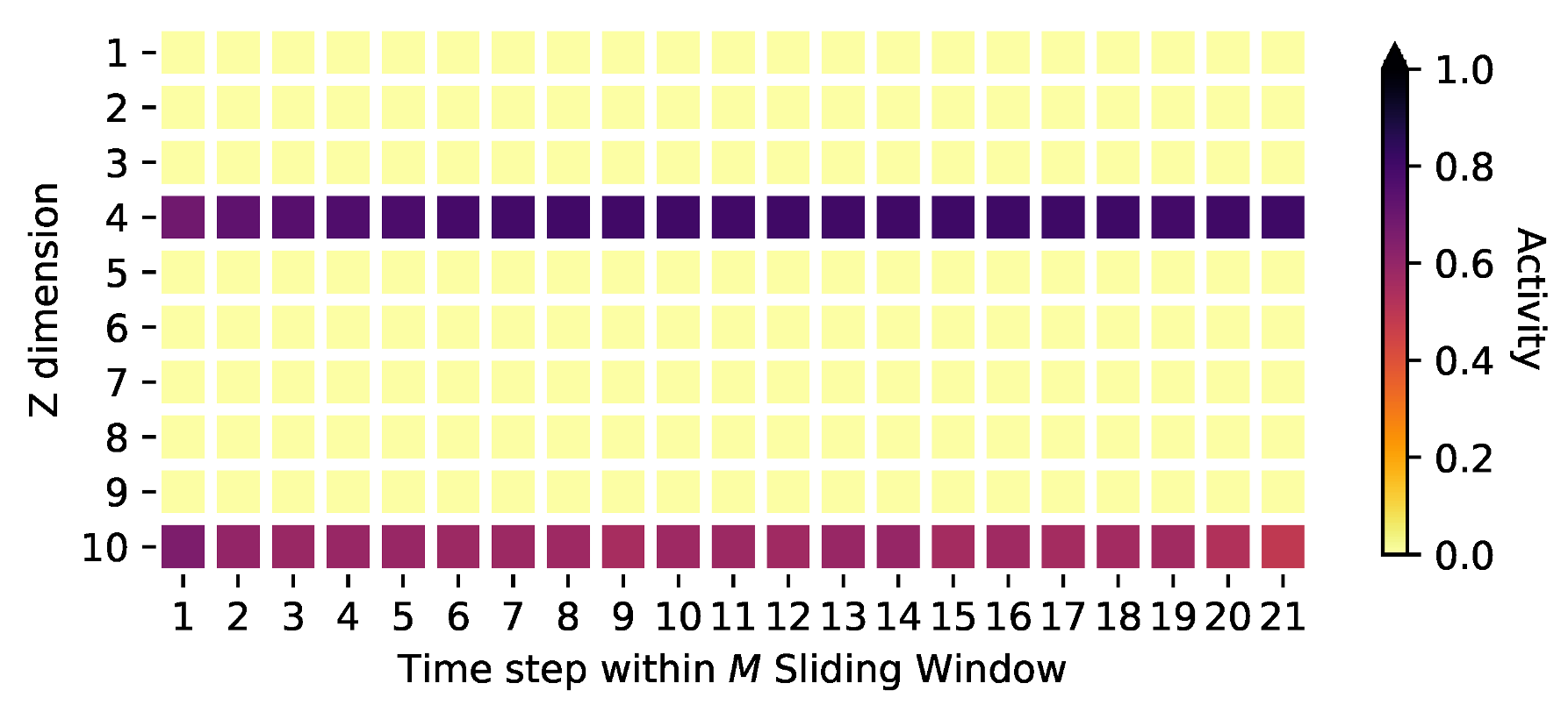
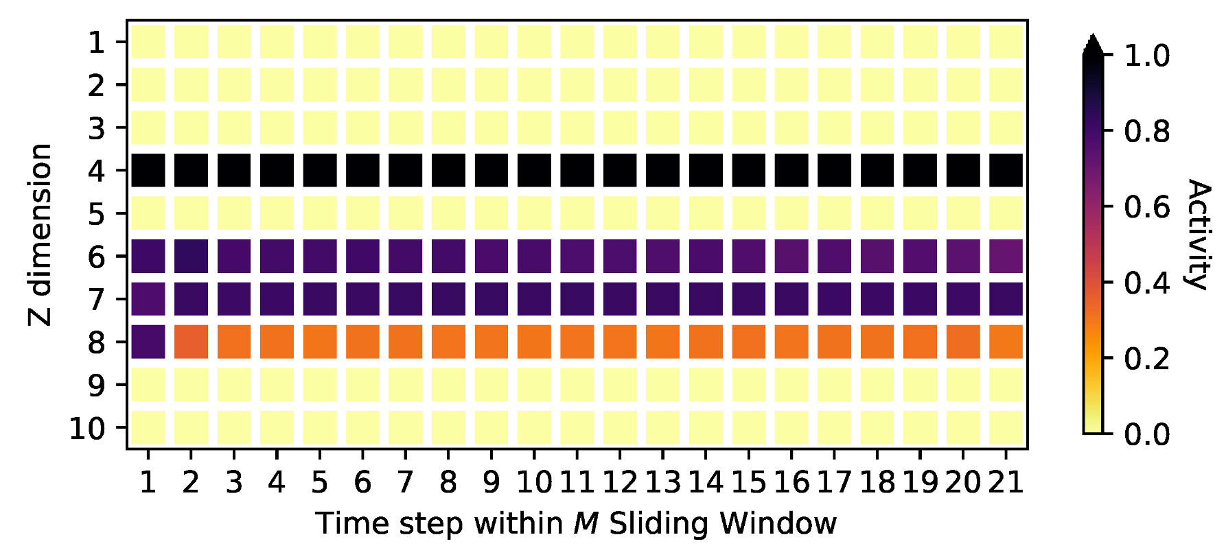
Appendix D. Activities on the Oscillating PCA Data Sets

For “oscillating PCA 5” and “oscillating PCA 10”, the model identifies two active dimensions through time, as can be seen in Figure A10 and Figure A11. In our point of view, this is not problematic, since the non-linearities of the artificial neural net can be the reason that fewer dimensions are needed to model the data appropriately. This can be observed in Table A8. Comparable scores are achieved for the Score Portfolio NLL. Furthermore, this can also be observed when we look at the fit of the model. For an excerpt of the first two dimensions, see Figure A12, Figure A13 and Figure A14.
Figure A10. The activity statistics for the “oscillating PCA 5” data. We consider sequences of size M = 21 as input. The graph shows the activity values of statistic (21) for the κ = 10 dimensional latent space.
Risks 11 00079 g0a10
Figure A11. The activity statistics for the “oscillating PCA 10” data. We consider sequences of size M = 21 as input. The graph shows the activity values of statistic (21) for the κ = 10 dimensional latent space.
Risks 11 00079 g0a11
Table A8. The different fit scores for the model TempVAE on the “oscillating PCA” datasets. Comparable scores are achieved for the Score Portfolio NLL. The multivariate scores are not comparable, as the structure of the data is not Gaussian.
ScoreOsc. PCA 2Osc. PCA 5Osc. PCA 10
TempVAE Portfolio NLL−5.21−5.77−4.80
Figure A12. The kernel density estimated distribution of the first two dimensions R t , 1 : 2 of the “oscillating PCA 2” data. On the left, we see the TempVAE model, and on the right, we see the historical data.
Risks 11 00079 g0a12
Figure A13. The kernel density estimated distribution of the first two dimensions R t , 1 : 2 of the “oscillating PCA 5” data. On the left, we see the TempVAE model, and on the right, we see the historical data.
Risks 11 00079 g0a13
Figure A14. The kernel density estimated distribution of the first two dimensions R t , 1 : 2 of the “oscillating PCA 10” data. On the left, we see the TempVAE model, and on the right, we see the historical data.
Risks 11 00079 g0a14

Appendix E. Activities on the Stock Market Data and Model Adaptions for High-Dimensional Data

In Figure A15 and Figure A16, we see the activities for the 22 dimensional “DAX” data and the 397 dimensional “S&P500” data.
Figure A15. The activity statistics for the “DAX” data. We consider sequences of size M = 21 as input. The graph shows the activity values of statistic (21) for the κ = 10 dimensional latent space.
Risks 11 00079 g0a15
As the dimension of the data increased by a factor of 18 compared to the the other datasets in Section 4.1, we adjust the model implementation. For the RNN layers in (9), (14), (15) and (16) we choose dimension 80, for the RNN layer in (6) we choose dimension 16. For the MLPs in (13), (5) and (8), we keep the two hidden layers and choose dimensions 60 and 30 for the first and second layer, respectively. Furthermore, we reduce the initial learning rate to 1e-4 and change the β -annealing steps from 20 to 100.
Figure A16. The activity statistics for the “S&P500” data. We consider sequences of size M = 21 as input. The graphs shows the activity values of statistic (21) for the κ = 10 dimensional latent space.
Risks 11 00079 g0a16

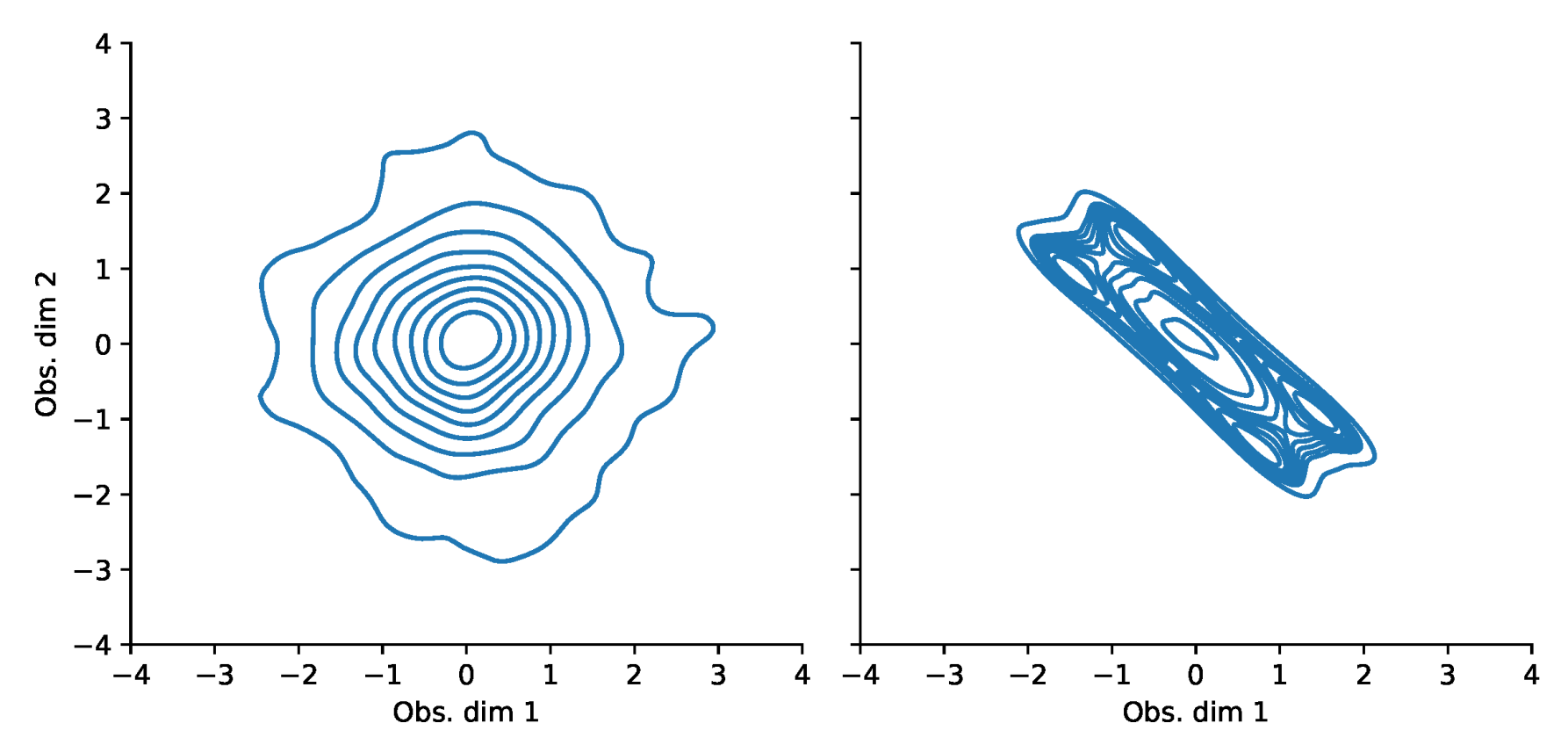
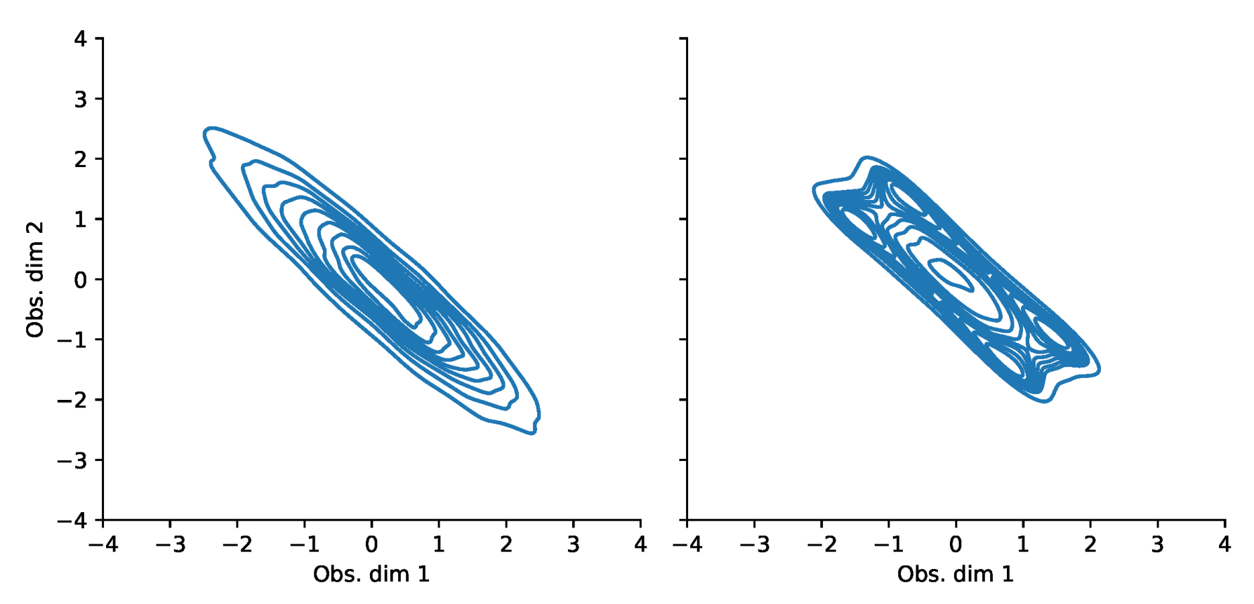
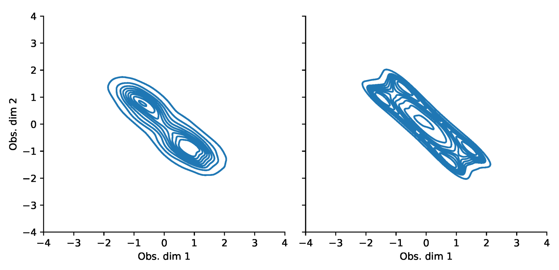
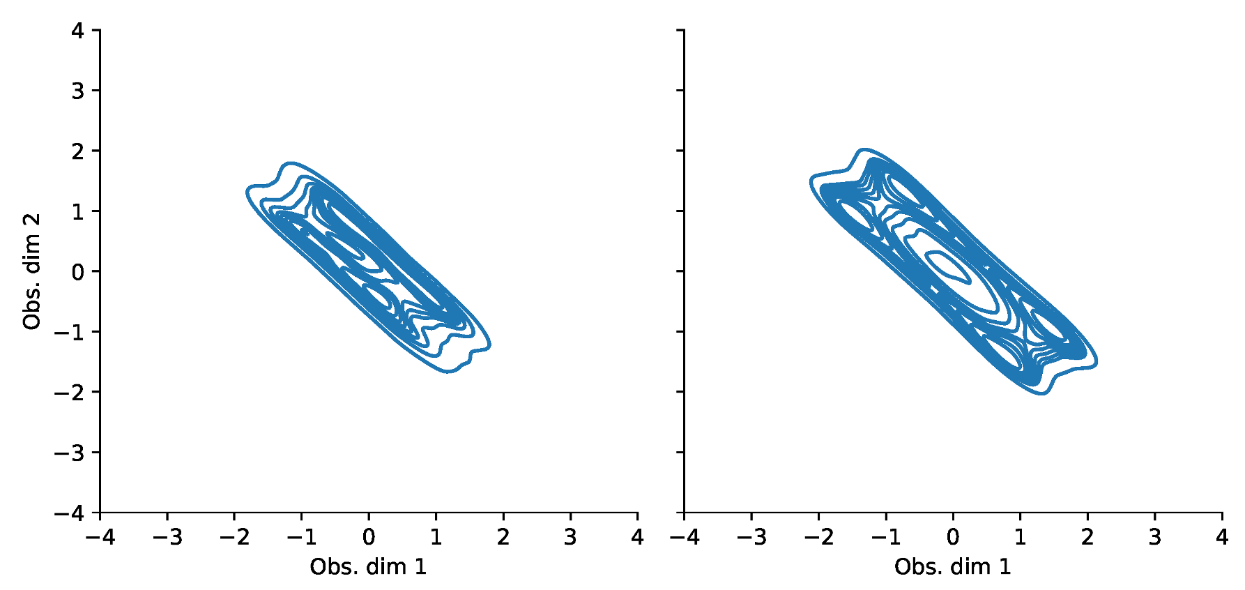
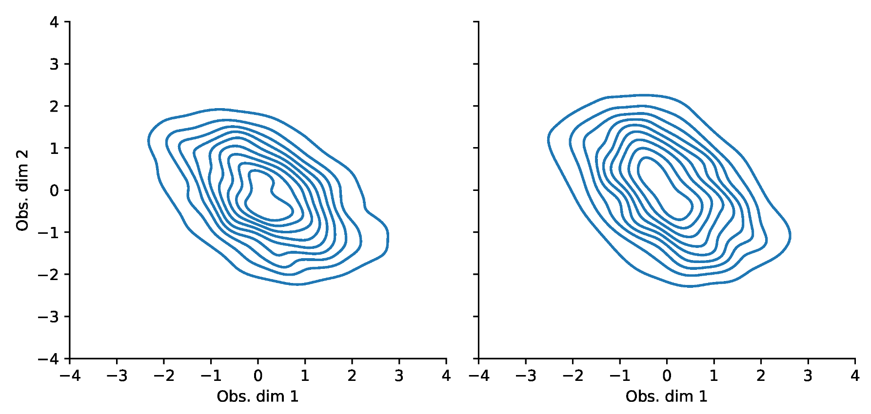
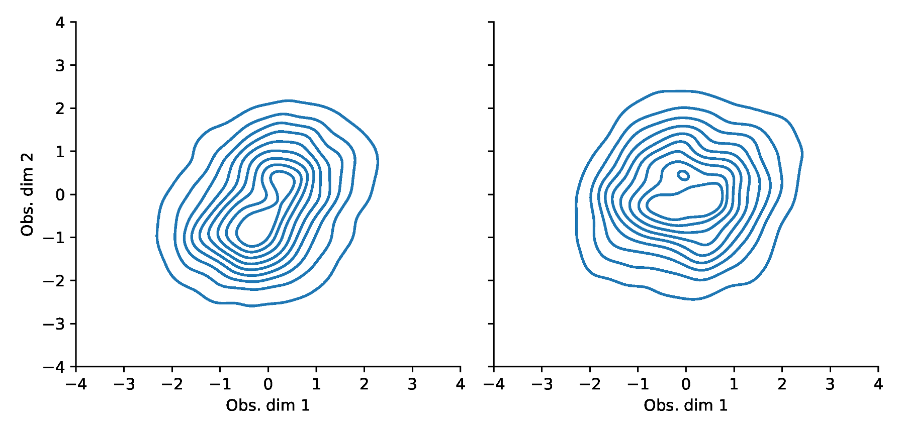
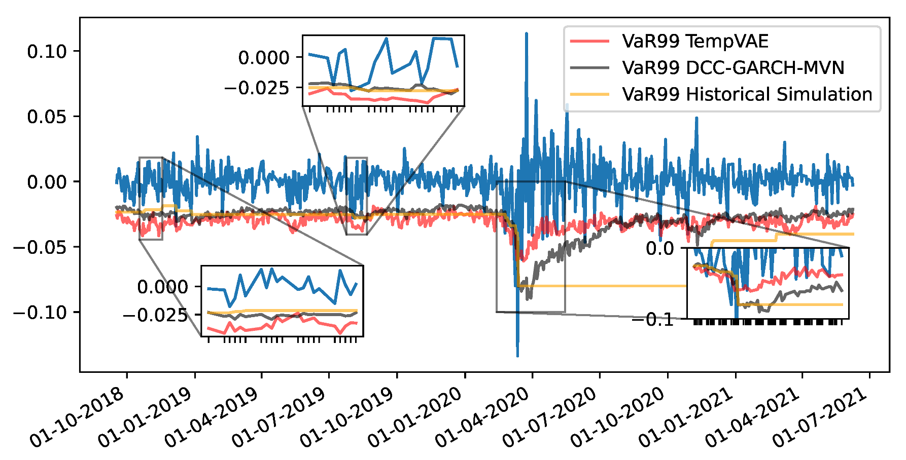
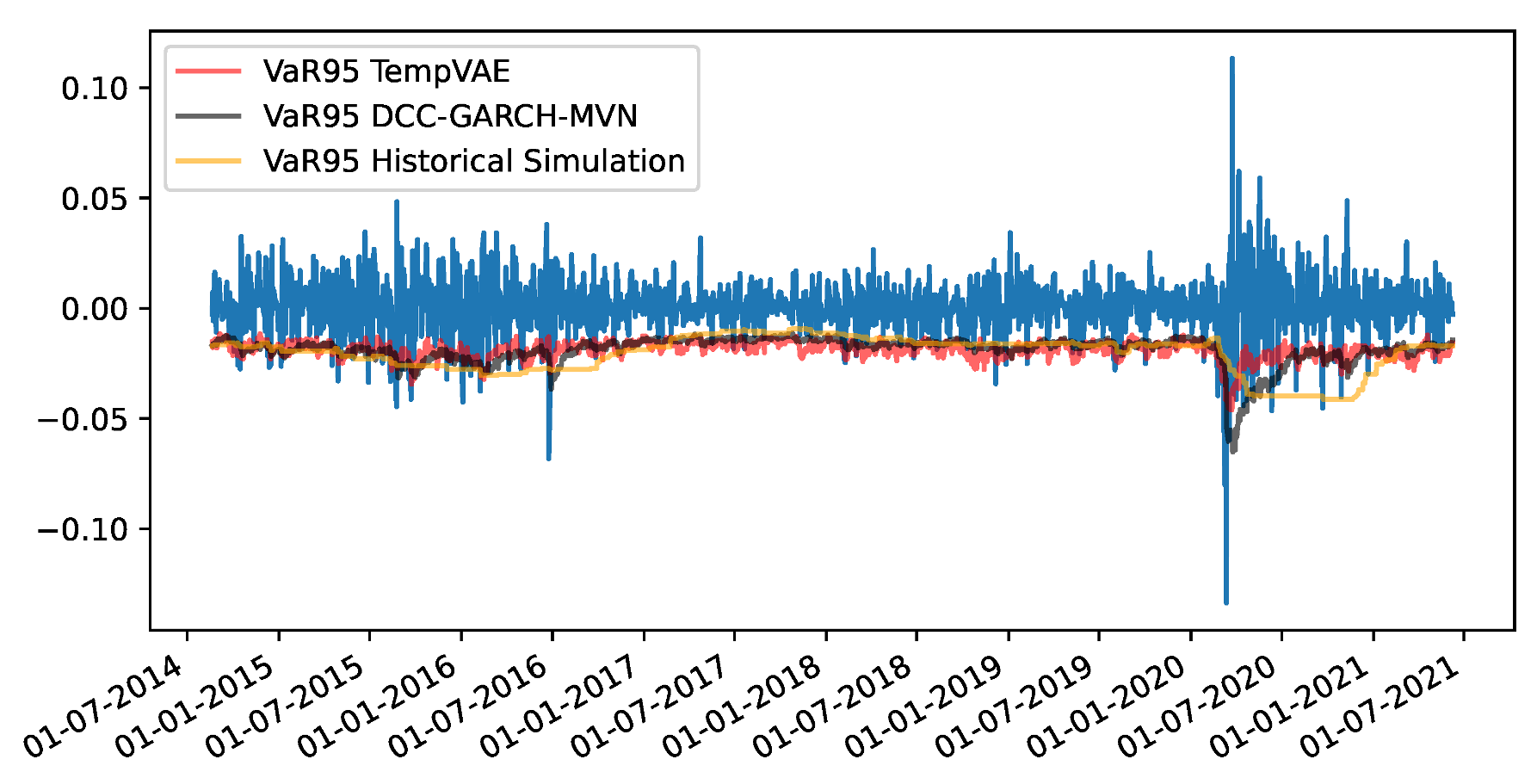
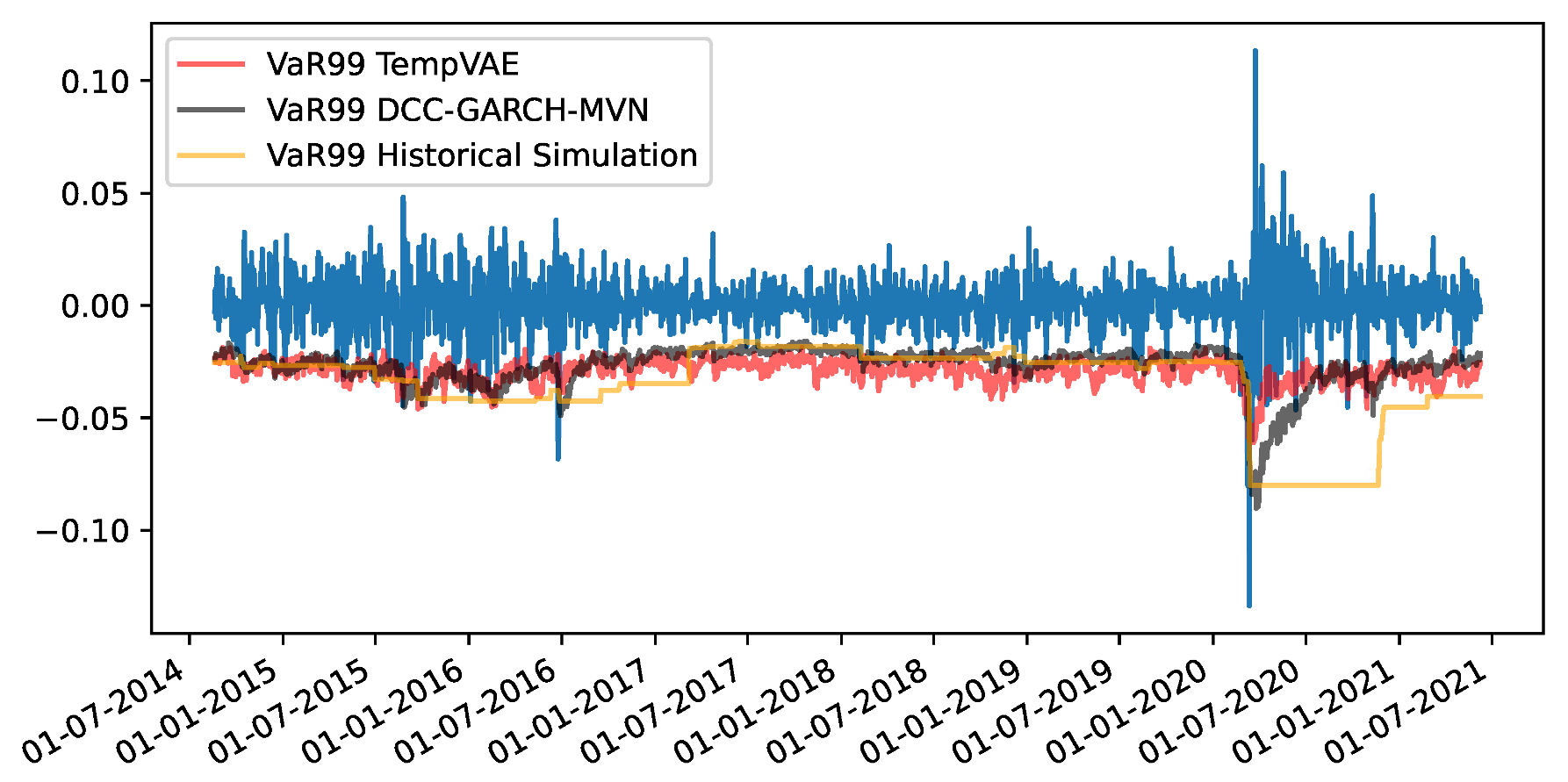
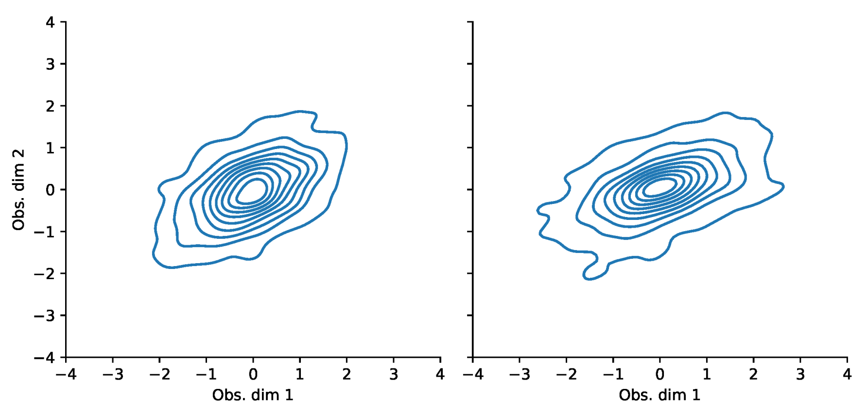
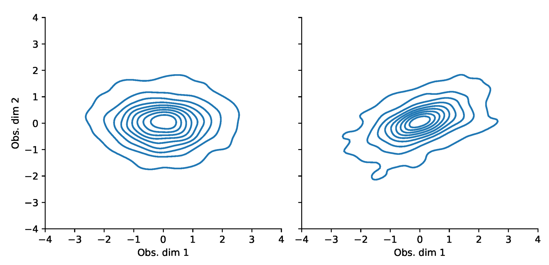
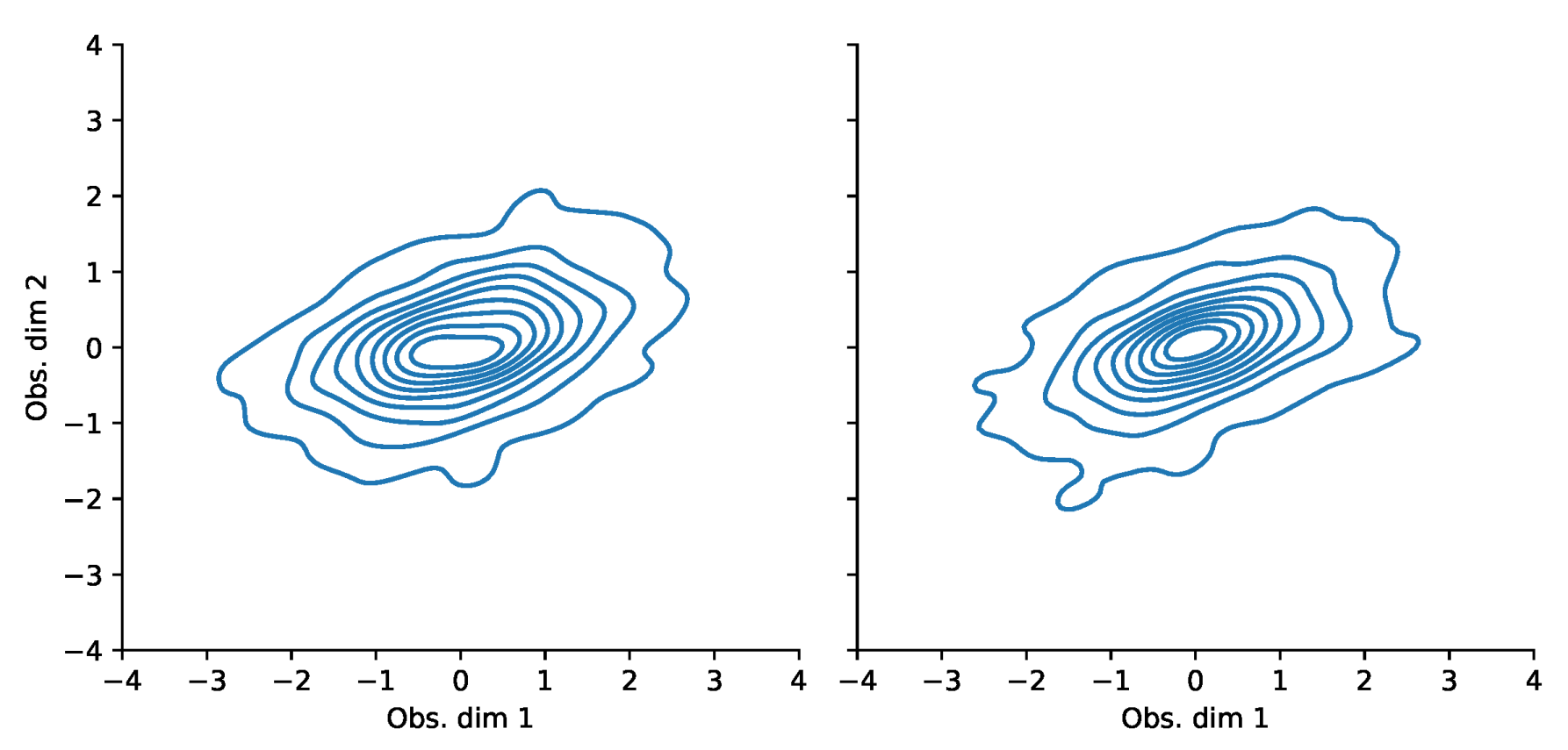
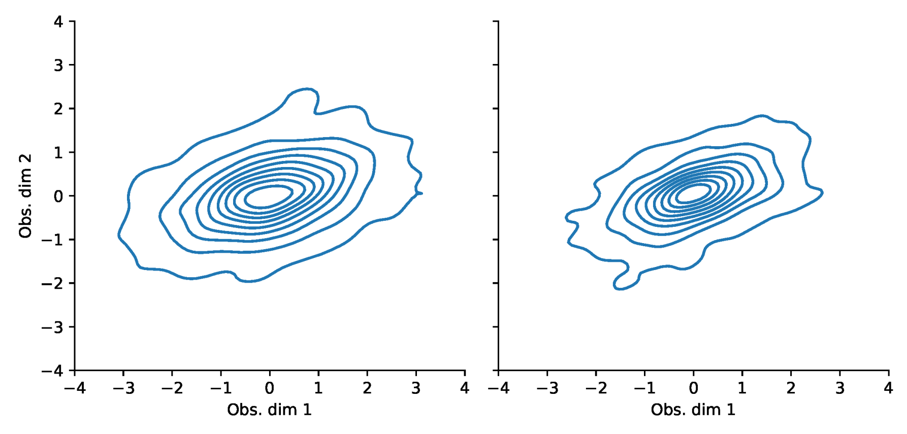
Appendix F. VaR and Scatterplots

In this section, we will show some further VaR path plots for the models TempVAE, HS and DCC-GARCH-MVN. For this, see Figure A17, Figure A18 and Figure A19.
Furthermore, we provide scatterplots for the first two dimensions of the different models used for the VaR estimation in Figure A20, Figure A21, Figure A22 and Figure A23.
Figure A17. The VaR99 estimates for the models TempVAE, DCC-GARCH-MVN and HS on a fraction of the test data.
Risks 11 00079 g0a17
Figure A18. The VaR95 estimates for the two models TempVAE, DCC-GARCH-MVN and HS on the whole test data.
Risks 11 00079 g0a18
Figure A19. The VaR99 estimates for the two models TempVAE, DCC-GARCH-MVN and HS on the whole test data.
Risks 11 00079 g0a19
Figure A20. The kernel density estimated distribution of the first two dimensions R t , 1 : 2 of the “DAX” data. On the left, we see the TempVAE model and on the right, we see the historical data.
Risks 11 00079 g0a20
Figure A21. The kernel density estimated distribution of the first two dimensions R t , 1 : 2 of the “DAX” data. On the left, we see the GARCH model, and on the right, we see the historical data.
Risks 11 00079 g0a21
Figure A22. The kernel density estimated distribution of the first two dimensions R t , 1 : 2 of the “DAX” data. On the left, we see the DCC-GARCH-MVN model, and on the right, we see the historical data.
Risks 11 00079 g0a22
Figure A23. The kernel density estimated distribution of the first two dimensions R t , 1 : 2 of the “DAX” data. On the left, we see the DCC-GARCH-MVt model, and on the right, we see the historical data.
Risks 11 00079 g0a23

Notes

1
i.e., the fact that drift parameters are notoriously hard to estimate while volatility parameters are much easier to obtain.
2
E.g., p ( R | Z ) = t = 1 T p ( R t | R 1 : t 1 , Z 1 : t ) .
3
Then, the assumption is p θ ( Z ) = t = 1 T p θ ( Z t ) , with p θ ( Z t ) N ( 0 , I ) for all t = 1 , , T .
4
This is common practice when modeling financial data as the increments of the log-stock prices are typically assumed to be independent (or at least uncorrelated) while the price increments are definitely not. For our later application in risk management (the VaR estimation), we therefore transform the log-return forecasts of the models to actual returns by using R t , i nonlog : = exp R t , i 1 ) to model the extremes in the data adequately.
5
The benchmark models are note feasible on the “S&P500” data due to a too high dimension.
6
We consider a time window of 180 days.
7
Note that usually one can calculate the VaR estimates for GARCH models analytically. But as we apply a non-linear transform of the modeled log-returns (see expression (24)) this task is not trivially performed.
8
Indeed, we could get the fractions of mispredictions correct by always predicting the VaR as for the initial fractions of the predictions and then equal to 1 (i.e., a total loss). Of course, this is no reasonable predictor!

References

  1. Arian, Hamidreza, Mehrdad Moghimi, Ehsan Tabatabaei, and Shiva Zamani. 2020. Encoded Value-at-Risk: A Predictive Machine for Financial Risk Management. arXiv arXiv:2011.06742. [Google Scholar] [CrossRef]
  2. Arimond, Alexander, Damian Borth, Andreas G. F. Hoepner, Michael Klawunn, and Stefan Weisheit. 2020. Neural Networks and Value at Risk. SSRN Electronic Journal, 20–7. [Google Scholar] [CrossRef]
  3. Bayer, Justin, and Christian Osendorfer. 2014. Learning Stochastic Recurrent Networks. arXiv arXiv:1411.7610v3. [Google Scholar]
  4. Bishop, Christopher M. 2006. Pattern Recognition and Machine Learning. Berlin/Heidelberg: Springer. [Google Scholar]
  5. Bollerslev, Tim. 1986. Generalized Autoregressive Conditional Heteroskedasticity. Journal of Econometrics 31: 307–27. [Google Scholar] [CrossRef]
  6. Bowman, Samuel R., Luke Vilnis, Oriol Vinyals, Andrew M. Dai, Rafal Jozefowicz, and Samy Bengio. 2015. Generating Sentences from a Continuous Space. In CoNLL 2016—20th SIGNLL Conference on Computational Natural Language Learning, Proceedings. Berlin: Association for Computational Linguistics (ACL), pp. 10–21. [Google Scholar]
  7. Burda, Yuri, Roger Grosse, and Ruslan Salakhutdinov. 2016. Importance Weighted Autoencoders. Paper presented at International Conference on Learning Representations, ICLR, San Juan, PR, USA, May 2–4. [Google Scholar]
  8. Chen, Luyang, Markus Pelger, and Jason Zhu. 2023. Deep Learning in Asset Pricing. Management Science. (online first). [Google Scholar] [CrossRef]
  9. Chen, Xiaoliang, Kin Keung Lai, and Jerome Yen. 2009. A statistical neural network approach for value-at-risk analysis. Paper presented at 2009 International Joint Conference on Computational Sciences and Optimization, CSO 2009, Sanya, China, April 24–26; vol. 2, pp. 17–21. [Google Scholar] [CrossRef]
  10. Cho, Kyunghyun, Bart Van Merriënboer, Caglar Gulcehre, Dzmitry Bahdanau, Fethi Bougares, Holger Schwenk, and Yoshua Bengio. 2014. Learning Phrase Representations using RNN Encoder-Decoder for Statistical Machine Translation. Paper presented at EMNLP 2014—2014 Conference on Empirical Methods in Natural Language Processing, Doha, Qatar, October 25–29; pp. 1724–34. [Google Scholar] [CrossRef]
  11. Chung, Junyoung, Kyle Kastner, Laurent Dinh, Kratarth Goel, Aaron C. Courville, and Yoshua Bengio. 2015. A Recurrent Latent Variable Model for Sequential Data. Advances in Neural Information Processing Systems 28: 2980–8. [Google Scholar]
  12. Engle, Robert. 2012. Dynamic Conditional Correlation. Journal of Business & Economic Statistics 20: 339–50. [Google Scholar] [CrossRef]
  13. Fatouros, Georgios, Georgios Makridis, Dimitrios Kotios, John Soldatos, Michael Filippakis, and Dimosthenis Kyriazis. 2022. DeepVaR: A framework for portfolio risk assessment leveraging probabilistic deep neural networks. Digital Finance 2022: 1–28. [Google Scholar] [CrossRef] [PubMed]
  14. Fraccaro, Marco, Simon Kamronn, Ulrich Paquet, and Ole Winther. 2017. A Disentangled Recognition and Nonlinear Dynamics Model for Unsupervised Learning. Advances in Neural Information Processing Systems 30: 3602–11. [Google Scholar]
  15. Fraccaro, Marco, Søren Kaae Sønderby, Ulrich Paquet, and Ole Winther. 2016. Sequential Neural Models with Stochastic Layers. Advances in Neural Information Processing Systems 29: 2207–15. [Google Scholar]
  16. Ghalanos, Alexios. 2019. rmgarch: Multivariate GARCH models. R Package Version 1.3-7. Available online: https://cran.microsoft.com/snapshot/2020-04-15/web/packages/rmgarch/index.html (accessed on 1 December 2022).
  17. Girin, Laurent, Simon Leglaive, Xiaoyu Bie, Julien Diard, Thomas Hueber, and Xavier Alameda-Pineda. 2020. Dynamical Variational Autoencoders: A Comprehensive Review. Foundations and Trends in Machine Learning 15: 1–175. [Google Scholar] [CrossRef]
  18. Goyal, Anirudh, Alessandro Sordoni, Marc-Alexandre Côté, Nan Rosemary Ke, and Yoshua Bengio. 2017. Z-Forcing: Training Stochastic Recurrent Networks. Advances in Neural Information Processing Systems 2017: 6714–24. [Google Scholar]
  19. He, Kaiming, Xiangyu Zhang, Shaoqing Ren, and Jian Sun. 2015. Delving Deep into Rectifiers: Surpassing Human-Level Performance on ImageNet Classification. Paper presented at The IEEE International Conference on Computer Vision (ICCV), Santiago, Chile, December 7–13. [Google Scholar]
  20. Kingma, Diederik P., and Jimmy Lei Ba. 2015. Adam: A method for stochastic optimization. Paper presented at 3rd International Conference on Learning Representations, ICLR, San Diego, CA, USA, May 7–9. [Google Scholar]
  21. Kingma, Diederik P., and Max Welling. 2014. Auto-Encoding Variational Bayes. Paper presented at 2nd International Conference on Learning Representations, ICLR, Banff, AB, Canada, April 14–16; Technical Report. Available online: https://arxiv.org/pdf/1312.6114.pdf (accessed on 1 December 2022).
  22. Kingma, Diederik P., Danilo J. Rezende, Shakir Mohamed, and Max Welling. 2014. Semi-supervised Learning with Deep Generative Models. Paper presented at the 27th International Conference on Neural Information Processing Systems, Montreal, QC, Canada, December 8–13. [Google Scholar]
  23. Krishnan, Rahul, Uri Shalit, and David Sontag. 2017. Structured Inference Networks for Nonlinear State Space Models. Paper presented at AAAI Conference on Artificial Intelligence, San Francisco, CA, USA, February 4–9; vol. 31. [Google Scholar]
  24. Laloux, Laurent, Pierre Cizeau, Marc Potters, and Jean-Phillippe Bouchard. 2000. Random Matrix and Financial Correlations. International Journal of Theoretical and Applied Finance 3: 391–97. [Google Scholar] [CrossRef]
  25. Liu, Yan. 2005. Value-at-Risk Model Combination Using Artificial Neural Networks. In Emory University Working Paper Series. Atlanta: Emory University. [Google Scholar]
  26. Luo, Rui, Weinan Zhang, Xiaojun Xu, and Jun Wang. 2018. A Neural Stochastic Volatility Model. Paper presented at AAAI Conference on Artificial Intelligence, New Orleans, LA, USA, February 2–7; vol. 32. [Google Scholar]
  27. Rezende, Danilo Jimenez, Shakir Mohamed, and Daan Wierstra. 2014. Stochastic Backpropagation and Approximate Inference in Deep Generative Models. Paper presented at the 31 st International Conference on Machine Learning, Beijing, China, June 21–26; pp. 1278–86. [Google Scholar]
  28. Sarma, Mandira, Susan Thomas, and Ajay Shah. 2003. Selection of Value-at-Risk Models. Journal of Forecasting 22: 337–58. [Google Scholar] [CrossRef]
  29. Sicks, Robert, Ralf Korn, and Stefanie Schwaar. 2021. A Generalised Linear Model Framework for β-Variational Autoencoders based on Exponential Dispersion Families. Journal of Machine Learning Research 22: 1–41. [Google Scholar]
  30. Xu, Xiuqin, and Ying Chen. 2021. Deep Stochastic Volatility Model. arXiv arXiv:2102.12658. [Google Scholar]
Figure 1. The dependency structure of the generative model. Realizations of Z influence the realizations of R as well as all future realizations of R and Z. The Gaussian distribution parameters from the MLP as well as the sampling are represented by the dashed lines. Furthermore, information of former time points is propagated through the RNN hidden states h . r and h . z .
Risks 11 00079 g001
Figure 2. The first 100 steps of two oscillating signals. The two signals have different amplitude, frequency and origin.
Risks 11 00079 g002
Figure 3. The activity statistics for the “Noise” data. We consider sequences of size M = 21 as input. The graph shows the activity values of statistic (21) for the κ = 10 dimensional latent space.
Risks 11 00079 g003
Figure 4. The activity statistics for the “Oscillating PCA 2” data. We consider sequences of size M = 21 as input. The graph shows the activity values of statistic (21) for the κ = 10 dimensional latent space.
Risks 11 00079 g004
Figure 5. The VaR95 estimates for the two models TempVAE, DCC-GARCH-MVN and for HS on a fraction of the test data. The blue line shows the original return data.
Risks 11 00079 g005
Table 1. Fit scores for models TempVAE, GARCH and two multivariate GARCH. In all cases, lowest is best.
ModelDiagonal NLLNLLPortfolio NLL
GARCH22.7622.84−0.51
TempVAE25.7920.35−3.04
DCC-GARCH-MVN25.0318.69−3.07
DCC-GARCH-MVt25.4419.17−3.05
Table 2. The table displays the values (all of these have to be multiplied by 10 2 ) of the RLF scores as well as the average number of exceedances for the VaR95 and the VaR99 within the test set. For the RLF values, lowest is best. For the average exceedances, the respective quantile level assumption is the optimal value. Hence, for VaR95, the best value is 5, and for VaR99, the best value is 1.
ModelRLF95RLF99AE95AE99
GARCH44.4732.3524.317.8
TempVAE12.645.964.81.3
DCC-GARCH-MVN13.157.105.42.1
DCC-GARCH-MVt10.234.143.90.6
HS14.577.435.11.3
Disclaimer/Publisher’s Note: The statements, opinions and data contained in all publications are solely those of the individual author(s) and contributor(s) and not of MDPI and/or the editor(s). MDPI and/or the editor(s) disclaim responsibility for any injury to people or property resulting from any ideas, methods, instructions or products referred to in the content.

