Abstract
This paper introduces and studies a new family of diffusion models for stock prices with applications in portfolio optimization. The diffusion model combines (stochastic) elasticity of volatility (EV) and stochastic volatility (SV) to create the SEV-SV model. In particular, we focus on the SEV component, which is driven by an Ornstein–Uhlenbeck process via two separate functional choices, while the SV component features the state-of-the-art 4/2 model. We study an investment problem within expected utility theory (EUT) for incomplete markets, producing closed-form representations for the optimal strategy, value function, and optimal wealth process for two different cases of prices of risk on the stock. We find that when EV reverts to a GBM model, the volatility and speed of reversion of the EV have a strong impact on optimal allocations, and more aggressive (bull markets) or cautious (bear markets) strategies are hence recommended. For a model when EV reverts away from GBM, only the mean reverting level of the EV plays a role. Moreover, the presence of SV leads mainly to more conservative investment decisions for short horizons. Overall, the SEV plays a more significant role than SV in the optimal allocation.
1. Introduction
The literature on optimal investment within expected utility began in the late 60s, where the risky asset price was assumed as a geometric Brownian motion (GBM); see the celebrated work of Merton (1969). Since then, many empirical studies have shown that this simple model cannot properly fit real market data. The main drawback is that the GBM does not capture implied volatility smile/skew effects from option prices.
To address its limitation, a simple extension of the GBM is the so-called local-volatility constant elasticity of variance (CEV) model, originally proposed by Cox (1975) and Cox and Ross (1976) as an alternative diffusion process for European option pricing. Compared with the GBM, the merits of the CEV model are that the volatility rate correlates with the risky asset price, known as the leverage effect, and empirical biases such as volatility smile can be better captured. Beckers (1980), MacBeth and Merville (1980), and Emanuel and MacBeth (1982) presented some theoretical arguments as well as empirical evidence to support volatility changing with the stock price and a negative elasticity factor. The main application of the CEV process has been on derivative pricing (see, for instance, Cox 1996; Davydov and Linetsky 2001; Lo et al. 2000; Yuen et al. 2001). As for portfolio optimization, Gao (2009) explored the optimal investment problem for defined contributions (DC) retirement plans under a CEV model. The author derived the respective explicit solutions for the CRRA and CARA utility functions by applying the stochastic optimal control, power transformation, and variable change technique.
As documented in (Kim et al. 2014), however, one main disadvantage in the CEV framework is that volatilities and underlying risky asset prices are perfectly correlated. Much evidence currently exists of volatilities being correlated with but decoupled from stock prices (e.g., implied volatility structures and trading of volatility indexes). These stylized facts cannot be captured within constant elasticity of volatility models. To overcome this restriction, some researchers have proposed a time-varying elasticity parameter (see Ghysels et al. 1996; Harvey 2001). In particular, Kim et al. (2014) introduced an extension of the CEV model named: “stochastic elasticity of variance” (SEV). The authors relaxed the time deterministic elasticity assumption by allowing the elasticity to vary randomly, and hence decoupled the movements of implied volatility from the risky asset prices. No attempt at portfolio optimization for SEV models is known to the authors.
In a separate branch of the literature, stochastic volatility (SV) models are a natural extension to the GBM and are capable of generating random volatility correlated with the stock price. The 4/2 model is a new popular stochastic volatility (SV) model that was first introduced by (Grasselli 2017). It combines the classic (Heston 1993) i.e., the 1/2 (Heston) model and the 3/2 model of (Heston 1997) and (Platen 1997). By combining the two, the 4/2 model inherits the benefits of both 1/2 and 3/2 models while bringing additional benefits such as an instantaneous volatility uniformly bounded away from zero and closed-form solutions for pricing derivatives (see, e.g., Cui et al. 2017a, 2017b, 2018). In terms of portfolio optimization, Kraft (2005), Chacko and Viceira (2005), and Boguslavskaya and Muravey (2016) provided closed-form solutions and asymptotic expansions for various SV models. More recently, Cheng and Escobar-Anel (2021) solved the expected utility problem for the 4/2 SV model in the family of CRRA utilities, while (Cheng and Escobar-Anel 2022) extended it to HARA. They derived analytical representations of the optimal investment strategies, optimal wealth, and value function.
The separate benefits of both SEV and SV models tell an story of how the log of the instantaneous volatility of stock returns depend on the stock itself (CEV) and also on external factors (SEV, SV). Together, the presence of SEV and SV components imply that the percentage change of volatility depends linearly on the percentage change in stock prices (i.e., elasticity of volatility), with the caveat that the coefficients in this relation are time dependent and random. Some researchers have already contributed to working with a hybrid structure but almost entirely on the topic of pricing derivatives. For instance, Choi et al. (2013) introduced a hybrid model built as a CEV multiplied by a stochastic volatility term driven by a fast mean-reverting Ornstein–Uhlenbeck process. Moreover, Cao et al. (2021) applied the hybrid model (SVCEV) to pricing a variance swap. As for portfolio optimization, Gao (2010) works with a CEV-1/2 model, leading to an approximated solution for a CRRA utility. However, the application of a hybrid structure that combines the SEV and 4/2 models for investment problems has not been studied yet.
In this paper, we introduce a new hybrid model that combines the properties of both the SEV and 4/2 processes. We do so by introducing an instantaneous volatility of the form for some constants , where is the CIR factor, and is driven by an OU process . We denote this hybrid structure as the SEV-4/2 model.
The main contributions of the paper are as follows:
- We define a new, richer model capturing both stochastic elasticity of volatility and stochastic volatility.
- We study two sub-models arising from the way in which the OU process relates to the elasticity of volatility . We use estimates of the 4/2 model as per (Cheng and Escobar-Anel 2021) and estimates for the SEV as per (Kim et al. 2015) for further analyses.
- In closed-form optimal investment, we find optimal wealth and value function for a risk-averse investor within expected utility theory, for two choices of prices of risk (MPR). Our setting is different from that of (Gao 2010).
- We show the impact of the new parameters, namely , and , on the optimal allocation. For this, we select and fix the paths of the processes representing states of the market, i.e., increasing prices (bull market), a decreasing path (bear market), and stable prices (normal market conditions).
- We also compare the solution in the absence of SV to separate the effects of SEV from those of SV.
The structure of this paper is as follows: Section 2 introduces the SEV-4/2 model and some properties. In Section 3, we derive closed-form solutions for the optimal strategy, wealth, and value function for two choices of prices of risk (MPR). The parametric and numerical settings are discussed in Section 4, and we analyze the sensitivity for two cases in Section 5: (1) the interaction of SEV and SV processes and (2) the absence of SV process. Concluding remarks are provided in Section 6.
2. Material and Methods: Model Formulation and Properties
Assume that a financial market consists of one risk-free asset and one risky asset (i.e., stock). Let all the stochastic processes introduced in this paper be defined on a complete probability space , where is a right-continuous filtration generated by standard Brownian motions (BMs).
We assume that the price process of the risk-free asset evolves according to
where the interest rate r is assumed to be constant. The price processes of the risky asset follow the hybrid structure of what we define as an SEV-4/2 model:
where . The stochastic factors , evolve as follows:
with r, , , , , , ; ; ; ; and . Moreover, , and are initial values; , , are independent Brownian motions; and f is a bounded function of the hidden process ensuring that is well defined. In this setting, the MPR becomes ; therefore the cases and will be considered separately.
We consider two cases (the Gaussian function first, and the Arctan function second):
where is the Gaussian density function at y with mean and unit variance. In both cases, f lies in the practical region , which includes the GBM as a particular case. The functions could easily be modified to accommodate any bounded region for .
The presence of f is motivated by the formulation in Kim’s model (Kim et al. 2014). In that article, the authors define f as a function connecting/driving the elasticity via an Ornstein–Uhlenbeck (OU) process . The function f plays a key role in the behavior of the elasticity, and we consequently consider two cases to illustrate how this choice affects solutions to investment decisions.
On the one hand, the choice of the Gaussian function f in (5) is motivated by the possibility of the SEV model becoming close to the GBM () at times. In other words, we give credit to the GBM not only as a benchmark model but also as the natural state of the market under normal conditions. On the other hand, the choice of the Arctan function allows for to inherit the mean-reverting nature of directly. This can be seen from the almost linear behavior of Arctan around the mean-reverting level of . This second choice does not favor the GBM but rather a nonzero value for the long-term elasticity of volatility (i.e., the mean reversion level of , ).
In this hybrid structure, the variance driver and the elasticity are assumed to mean-revert around long-term values of and , with and reflecting the speed of mean reversion. Furthermore, is the volatility of volatility, and is the volatility of the stochastic volatility (SV) variance driver. At the same time, is the volatility of the elasticity of volatility (EV) driver . We also assume that the Feller condition holds true for the CIR process; i.e., , which prevents the process from becoming zero. In summary, is the volatility of the risky asset. The instantaneous correlation between the risky asset and the SV driver is . Note that no correlation exists between EV driver and or for the sake of simplicity.
The drift term in our model is different from that in the existent literature, but the diffusion term of our model embeds and connects popular stochastic volatility and the elasticity of volatility models in the literature. For example,
- = 0, , and —The celebrated SV Heston model (Heston 1993).
- , , and —The SV 3/2 model (Heston 1997).
- , , and —The SV stochastic volatility model (Grasselli 2017).
- , , , and —The constant elasticity of variance (CEV) model (see Cox 1975; Cox and Ross 1976).
- , , , and —The stochastic elasticity of variance (SEV) model (see Kim et al. 2014)
- and —The E-CEV model of (Gao 2010) and a particular case of the generalized SABR model in (Lions and Musiela 2007).
The SEV-4/2 model is inspired by a combination of the 4/2 SV in (Grasselli 2017) and the SEV of (Kim et al. 2014). The main motivation for both an SEV and an SV stems from the presentation in (Beckers 1980); our proposal means that the log of the instantaneous volatility of the stock return () can be expressed as follows:
where is the coefficient, and is the elasticity of volatility coefficient. Moreover, as explained in (Gao 2010), the CEV model leads to a perpetually declining volatility as the stock increases. To see this, note the instantaneous volatility is , and as the stock price increases over a long time, the instantaneous volatility will decrease to zero. This cannot be fixed entirely by creating an SEV. The best correction is to allow for an SV part in the instantaneous volatility.
Our model permits a risk-neutral pricing measure , which we identify via the change of measure1:
where , are independent standard Brownian motions under . This means, as per the notation in Equation (1), that and . Moreover, the processes under would read as follows:
Proposition 1.
The following conditions are needed for the change of measure in Equations (8)–(10) to be well defined2:
Proof.
The proof is presented in Appendix A.1. □
3. Results: Portfolio Problem and Solution
We invest in the stock and a cash account ; is the proportion of wealth allocated to the stock, and hence goes to cash. Using the self-financing condition, the wealth process for this investor under the real-world measure is given by
where is an initial wealth.
For all and , we assume that the SDE (16) has a pathwise unique solution under real-world measure . Let us define
where denote the conditional expectation.
To seek the optimal investment strategy , we maximize the expected utility of the terminal wealth
where is the power utility function
that is increasing and concave. is the value function, and denotes the space of admissible trading strategies. By using the dynamic programming approach, we obtain the form of optimal investment strategy and the Hamilton–Jacobi–Bellman (HJB) equation for this optimization problem, with boundary condition . The solution for the optimal strategy, terminal wealth, and value function are summarized in the next proposition.
Proposition 2.
The solution to problem (17) is provided next in two cases:
- Assume and hold. The value function (17) can be represented aswhere and are given bywith auxiliary parameters , , and , where . Then, the optimal strategy is given bywith defined by functions (5) and (6).Furthermore, the optimal wealth has the following dynamics under measurewith initial wealth .
- Furthermore, the optimal wealth has the following dynamics under real-world measurewith initial wealth .
Proof.
The proof is in Appendix A.2. □
It should be noted that although the optimal strategies in Equations (21) and (25) appear to be highly stochastic, the key value for an investor is the optimal number of shares allocated, as this would determine the transaction costs involved in keeping the optimal strategy. Our solution (Case 1) implies the following optimal number of shares:
In the case of a simple Merton (GBM) solution, this amounts to
which is also stochastic; therefore, one solution does not offer obvious benefits in terms of transaction costs compared to the other.
4. Results: Numerical Setting
The optimal solution to the portfolio problem, as per Section 3, depends on the parameters of the model and the evolution of the state variables/processes. Section 4 clarifies how the parameters are chosen and how the processes are simulated.
This section is organized as follows: Section 4.1 specifies the estimate values of the parameters in our model. We then discretize processes , , and for simulation in Section 4.2.
4.1. Parameter Value Selection
In our model, 12 parameters are required: r, , , a, b, , , , , , , and . Note that for simplicity, we assume that . We propose values for these parameters via a combination of two reliable sources on the embedded key models: the SEV and the 4/2.
- Values for the 4/2-related parameters , , in the SEV-4/2 modelOur model combines two models—the SEV and 4/2 models. The hybrid structure not only possesses new features but also inherits some characteristics of each of the two models. The parameters, , a, b, , , , and are inherited from the 4/2 model, and their estimates were already obtained by (Cheng and Escobar-Anel 2021). Table 1 displays these parameter values.
 Table 1. Estimates among the various models.
 - Values for the SEV-related parameters , , in the SEV-4/2 modelWe consider two approaches for these parameters based on the two bound functions f (see Equations (5) and (6)) connecting and .
- 2.1
- For the Gaussian function, we propose values of , , and for a baseline case and two other cases as follows in Table 2.
 Table 2. Estimation from the properties of the elasticity with the SEV-4/2 model.
 - 2.2
- For the Arctan function, we match the SEV part of our model to the SEV part of (Kim et al. 2015). Here, we call the SEV model in (Kim et al. 2015) as Kim’s model. To distinguish the parameters from our model’s parameters, we use a subscript K to denote parameters from Kim’s model. Let us recall that the stock price process can be expressed by the stochastic differential equation (SDE) in Kim’s model as follows:under a risk-neutral measure, where (interest rate) and (volatility coefficient) are positive constants, is a nonnegative stochastic process, and is a standard Brownian motion. Let (i.e., ) for convenience, and suppose that follows an Ornstein–Uhlenbeck process given by the solution to the SDE:where , , and are constants. From Figure 1 in (Kim et al. 2015), we know that the estimates of are . In addition, using the properties of OU processes, for we haveNow, with our model and notation, we getGiven the non-linear nature of f, we first perform a Taylor approximation for around . That is,Next, we match the properties of our approximated process and those of Kim’s process:Using formulae (31)–(33) yields , , and . Due to , it follows thatThus, for the Arctan function, we could propose values of , , and associated with Kim’s model for a new baseline case and two other cases, as listed in Table 3 below:
 Table 3. Estimation associated with Kim’s model for the SEV-4/2 model.
4.2. Model Discretization and Simulation
Our hybrid structure contains three processes: , , and . We apply the Euler–Maruyama scheme to simulate and . Discretization schemes of a CIR process are summarized in (Lord et al. 2010), Table 1. To simulate , we use the Higham and Mao method.
Consider a time horizon for . We subdivide the time interval into n subintervals of equal width . We keep track of the values of the corresponding three stochastic processes at each discrete-time point for . Within this setting, the approximation formulae are presented together with the steps in our simulations.
Accordingly, the discretization of and for simulations is as follows:
Prior to discretizing the underlying asset process, we first use the log return of the risky asset instead of the simple return of the asset. That is, using It’s lemma yields
where . Denote , and we then discretize to obtain
where is independent of t. Furthermore, the Gaussian triple has the following dependence
After simulating the processes , , and , we can produce the paths of optimal strategy as per Equation (21).
5. Results: Analysis of Optimal Investment Strategies
In this section, we analyze the effects of market parameters on the optimal stock allocation, especially the parameters of the hidden process driving the elasticity in our model, namely , , and . Throughout the section, unless otherwise stated, the basic parameters are given in Table 1, Table 2 and Table 3 in Section 4.1.
It should be noted that the optimal stock allocation depends explicitly on three underlying processes in our model: the stock price itself (), the driver of the stochastic elasticity of volatility (), and the driver of the stochastic volatility (). Therefore, the dependence of the optimal stock allocation on parameters is implicit; that is, the parameters impact the behavior of the underlying processes, hence impacting the optimal allocation decision.
To capture the influence of parameters fairly, we split the behavior of stock prices into three market states: bull market (increase in prices), bear market (decrease in prices), and normal market (stable prices). We then pick three () paths, , representing the bull mmrket path, the bear market path, and the normal market path, respectively, to fix the Brownian path generating such scenarios, where , . For these given paths, we explore the influence of the new parameters by comparing several different parametric choices. In other words, we consider only parameter changes, not changes in the path of the underlying noises.
Given that our model contains two components explaining instantaneous volatility (i.e., SEV and SV), we first explore the impact of the SEV parameters on the optimal allocation in the presence of both components (Section 5.1), and we then explore the impact of the same parameters in the absence of the SV component (Section 5.2).
5.1. Sensitivity to the Interaction of SEV and SV Processes
As in the previous section, the study is split into two parts, each corresponding to a functional representation of the elasticity of volatility.
- Gaussian function analysis. The figures in this analysis can be found in Appendix A.3.1.
- (a)
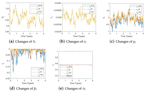
- Bull market conditions.The first three figures (Figure A1, Figure A2 and Figure A3 in Appendix A.3.1) illustrate the impact of parameters on the factors and the optimal stock allocation under the bull market path.We first study the impact of on the optimal stock allocation. We select three different values for : {0.5, 2, 10}. Figure A1a shows the behavior of the bull market path for the stock under these choices of . As anticipated, in such a bull market, a slower speed of reversion for generates more variation in and hence lower, more negative values (Figure A1d), leading to lower stock prices (compared with a faster reversion).Figure A1b shows no impact of parameters on as expected, while Figure A1c,d confirm the changes in speed of reversion for and , respectively.The optimal stock allocation in Figure A1e demonstrates a similar behavior as : a slower mean reversion of allocation for that quickens as increases. A decrease in the speed of reversion leads to (1) larger fluctuation on the optimal allocation due to larger fluctuations in and (2) more aggressive investment due to more negative values for . Interestingly, the more aggressive investments are a result of not only higher stock prices but also a more negative elasticity of volatility (), which result from a slower speed of reversion in .Figure A2 focuses on the impact of three different : {−1, 0, 1}. Figure A2a reports the changes in the bull market path for the stock price. Due to the assumption , changes in create a shift on the mean reverting level of (Figure A2b), which is further cancelled out by the function in the transformation from to , leading to no changes in (Figure A2c) and therefore no impact on stock prices (Figure A2a). This parameter is also disconnected from . Figure A2c,d indicate that variations in away from 0 (i.e., lower, more negative values) lead to more aggressive stock allocations.Figure A3 targets the influence of , {0.1, 1, 5}, on optimal stock allocation for the bull market path. In this case, a larger volatility has a similar effect as a slower speed of reversion. Therefore, it creates larger variations on (Figure A3d), e.g., lower, more negative values and hence lower stock prices (Figure A3a). This leads to similar implications in terms of optimal stock allocation (Figure A3e): the higher , the more aggressive the investments in the stock price (even though stock prices would be lower in this bull market, Figure A3a).In summary, the consistent pattern among all these figures (bull market) is that larger deviations of from 0 lead to more aggressive stock allocations; these variations can be incited by larger values of and smaller values of . This phenomenon can be explained, in financial terms, by observing that a more negative beta implies smaller volatilities, which, combined with an increase in stock prices (bull market), lead to excellent market conditions and therefore more aggressive stock allocations.
- (b)
- Bear market conditions.The detailed analysis presented above can be extended concisely to the case of the bear market (Figure A4, Figure A5 and Figure A6 for , , and , respectively). Here, larger deviations of (away from 0) combined with a downturn in prices (bear market) lead to a more conservative stock allocation. The variation in is more pronounced with larger values of or smaller values of . In financial terms, this suggests that lower stock prices combined with larger volatilities lead to more conservative risky allocations.
- (c)
- Normal market conditions.The case of normal market conditions (Figure A7, Figure A8 and Figure A9 for , , and , respectively) behaves as expected. That is, allocations could increase or decrease depending on small fluctuations in prices and beta, with no clear pattern in terms of aggressive/conservative behavior. As anticipated, causes larger fluctuations in optimal allocation, with a smaller impact by and no impact of . The sharp downward movement in allocations in these figures toward the end of the horizon (from year 4 to 5) is due to the impact of the SV component (not observable in the figures in Section 5.2). This means that the SV component plays a larger role under normal market conditions than it does under bull and bear conditions.
- Arctan function analysis. The figures in this analysis can be found in Appendix A.3.2.
- (a)
- Bull market conditions.Figure A10, Figure A11 and Figure A12 illustrate the impact of parameters on the factors and the optimal stock allocation under the bull market path. We first study the impact of on the optimal stock allocation. We select three different values for . In this section, we present on the main observations.Figure A10a indicates no impact of on the behavior of the stock . This is because inherits the mean-reverting nature of via the Arctan function, which behaves almost linearly around the mean-reverting level. Figure A10c,d confirm the changes in speed of reversion for and , respectively.The optimal stock allocation, as depicted Figure A10e, shows a similar behavior to that of . An increase in the speed of reversion leads to larger fluctuations on the optimal allocation due to larger fluctuations in . The range of the fluctuation is small and mostly impacted by the SV component due to the sharp downward movement toward the end of the horizon.Figure A11 depicts the impact of . Changes in create significant shifts on the elasticity of volatility in Figure A11c, leading to lower stock prices in Figure A11a. These large changes in impact the optimal stock allocation, as shown in Figure A11d. A smaller long-term mean leads to a more negative and more aggressive optimal allocations. Interestingly, the more aggressive investments are not a result of higher stock prices but rather a more negative elasticity of volatility ().Figure A12 focuses on the impact of . Figure A12b,c confirm the changes in volatility for and , respectively. The latter shows very small variations on (Figure A12c) and therefore no impact on stock prices (Figure A12a). All of the above lead to almost no impact on the optimal allocation for various volatilities . Similarly to above, here the main impact stems from the SV component, as evidenced by the downward movement.In summary, on the one hand, changes in and have almost no impact on the optimal allocation, as the main source of influence is the SV component. On the other hand, the long-term mean plays a key role: the more negative it is, the more aggressive the stock allocations become. This phenomenon can be explained, in financial terms, as follows: a more negative implies smaller volatilities, which, combined with an increase in stock prices (bull market), lead to excellent market conditions and hence more aggressive stock allocations.
- (b)
- Bear market conditions.The detailed analysis presented above can be extended concisely to the case of the bear market (Figure A13, Figure A14 and Figure A15 for , , and , respectively). First of all, optimal allocation remain insensitive to changes in and . Secondly, larger deviations of (away from 0), which happens for large negative values of , combined with a downturn in prices (bear market) lead to a more conservative stock allocation. In financial terms, this tells us that lower stock prices combined with larger volatilities lead to more conservative risky allocations.
- (c)
- Normal market conditions.The case of normal market conditions (Figure A16, Figure A17 and Figure A18 for , , and , respectively), behaves as expected and similarly to the bear and bull cases in terms of and .However, here, we also observe that the smaller the , the farther the deviation of from zero and hence the less aggressive the investment strategy. This means normal market conditions behave like bear market conditions in terms of the impact of parameters.
5.2. Sensitivity in the Absence of the SV Process
In Section 5.1, we observed several sharp downward movements of allocations in Figure A6 under bear market conditions and in Figure A7, Figure A8 and Figure A9 under normal market conditions from years 4 to 5. In particular, similar behaviors become more significant under all market conditions (bull, bear, and normal) in the Arctan function analysis. This new section shows that the reason for that behavior is the stochastic volatility part. Here, we perform the analysis when only the SEV component is considered. To eliminate the SV component in the solution, we make converge to zero, thereby forcing to be .
The study is split into two parts, each corresponding to a functional representation of the elasticity of volatility, namely the Gaussian function, and the Arctan function. For each of these two functions, we explore the impact of parameters in bull, bear, and normal markets.
- Gaussian function analysis. The figures in this analysis can be found in Appendix A.4.1.
- (a)
- Bull market conditions.Figure A19, Figure A20 and Figure A21 in Appendix A.4.1 illustrate the impact of parameters on the stock price and the optimal stock allocation under the bull market path. Since the order of parameters and values is the same as in Section 5.1, we will not repeat the details here.Compared to Section 5.1–1(a), Figure A19a shows a similar behavior of the bull market path for the stock under various as the interaction of the SEV and SV processes, which highlights the low impact of the SV part on the stock behavior. The optimal stock allocation, depicted in Figure A19b, presents a similar behavior as that in Section 5.1–1(a). However, the slight difference is that the curve of optimal allocations has a small shift towards conservative allocations due to the absence of the SV component. The allocation becomes less aggressive than that in Section 5.1–1(a).Figure A20 demonstrates the impact of . The behaviors of and optimal allocation are similar to those in Section 5.1– 1(a). Again, the curve of optimal allocations has a small shift towards conservative allocations due to the absence of the SV component.Figure A21 depicts the influence of on optimal stock allocation. The lack of the SV component creates a small shift towards conservative allocations.The major difference in the absence of the SV component is that we observe minimum impact on , and the curve of optimal allocations is similar in shape but has a small shift towards conservative allocations.
- (b)
- Bear market conditions.The analysis presented above can be extended to the case of bear market for , , and (Figure A22, Figure A23 and Figure A24, respectively, in Appendix A.4.1). Here, we observe the same behavior as presented for the Gaussian function with SEV and SV (Section 5.1–1(b)): larger deviations of (away from 0) combined with a downturn in prices (bear market) lead to a more conservative stock allocation. The variation in is more pronounced with larger values in or smaller values in . In addition, the sharp down turn in optimal allocations at the end of year 5 is corrected when the SV component is eliminated.
- (c)
- Normal market conditions.The case of normal market conditions (Figure A25, Figure A26 and Figure A27 for , , and respectively) behaves as in the corresponding Section 5.1–1(c). The key observation is that the sharp downward movement in allocations in these figures toward the end of the horizon (from year 4 to 5) is corrected in the absence of the SV component. This means that the SV component plays a larger role under normal market conditions than it does under bull and bear conditions.
- Arctan function analysis. The figures in this analysis can be found in Appendix A.4.2.
- (a)
- Bull market conditions.Figure A28, Figure A29 and Figure A30 illustrate the impact of parameters on the factors and the optimal stock allocation under the bull market path. The order of parameters and values is the same as in Section 5.1 and Section 5.2, so we will not repeat the details here.We first analyze the impact of . The behavior of is similar to that in Section 5.1–2(a), but the optimal stock allocation (Figure A28b) shows a significantly different behavior than in Section 5.1–2(a). As fluctuations on the optimal allocation are mostly impacted by the SV component, almost no fluctuations occur in this case. The sharp downside movement toward the end of the horizon has also disappeared.Figure A29 depicts the impact of . Similar behaviors are observed as those in Section 5.1–2(a) for various . Additionally, due to the lack of the SV component, almost no fluctuations occur in optimal allocation, and the sharp downside movement toward the end of the horizon observed in Section 5.1–2(a) is corrected.Figure A30 illustrate on the impact of , which is minimal on stock prices and on the optimal allocation. Again, due to the lack of the SV component, the downward movement of allocations in Section 5.1–2(a) disappears.In summary, only has some impact on the optimal allocation, and the sharp downside movements toward the end of the horizon are corrected in all cases.
- (b)
- Bear market conditions.The bear market analysis is illustrated in Figure A31, Figure A32 and Figure A33. Here also, optimal allocation remains insensitive to changes in and . Larger deviations of (away from 0) occur for large negative values of , which combined with a downturn in prices (bear market), lead to a more conservative stock allocation. In the absence of the SV component, the fluctuations in optimal allocations are very small, and the sharp downside movement toward the end of the horizon, as in Section 5.1–2(b), is also eliminated.
- (c)
- Normal market conditions.The case of normal market conditions is depicted in Figure A34, Figure A35 and Figure A36. This behaves as in the corresponding Section 5.1–2(c). More interestingly, in the absence of the SV component, the fluctuations in optimal allocations are very small, and, as expected, the sharp downside movement toward the end of the horizon disappears.
6. Conclusions, Limitations and Future Research
This paper presents the first portfolio optimization analysis using a hybrid structure of the SEV and SV models. We obtained closed-form solutions for the optimal strategy, value function, and optimal wealth process within EUT for two choices of prices of risk. We also explored two sub-models arising from an Ornstein–Uhlenbeck driver for the elasticity of volatility.
Using three simulated paths, each capturing three key market states, bull, bear and normal, we analyze the impact of the three main new parameters (i.e., , , ) on the optimal stock allocation. This is done for two separate functions (i.e., a Gaussian and Arctan) describing the behavior of the SEV component.
When applying the Gaussian function, for both bull and bear markets, we see that changes in the elasticity factor (i.e., ) has remarkable impact on stock allocations. In particular, the larger the deviation of from zero, the more aggressive the optimal stock strategy in the bull market, and the more conservative the optimal strategy in the bear market. Large variations in can be incited by larger values of or smaller values of , while changes in do not affect the behaviors of , and therefore there is little influence on allocation. These observations confirm the practitioners view that small volatility combined with an increase in stock prices (bull market) would lead to an excellent investment environment (higher risky allocation), while large volatility combined with a decrease in stock prices (bear market) generate a bad market condition, and accordingly, investors should take a prudent and conservative strategy in their investment of stocks.
For the Arctan function, only variations in the long-term mean () played an important role on the optimal stock allocations in the case of bull and bear markets. That is, larger negative values of generate larger deviations of (away from 0), leading to more aggressively optimal stock strategy in bull financial markets; whereas, more conservatively optimal stock allocations would be recommended in bear financial markets.
Interestingly, in normal market conditions, no clear pattern in terms of aggressive/ conservative behavior on the optimal allocation was observed for both functions, arctan and Gaussian. This was due to the small fluctuations in stock prices and . We also notice that the presence of SV component incites a sharp downward movements in the optimal allocation toward short maturities, this is well-known in the SV literature.
Overall, we found that the SEV process plays a more significant role in optimal allocations than the SV component, with some of the new parameters playing a bigger role, depending on the functional representation for the SEV. This has implications to financial institutions and policy makers in terms of what are the relevant models and the important parameters to check in order to ensure safe investment decisions.
In terms of limitations and future horizons for research, the problem addressed in this paper (i.e., SEV-SV in EUT) shall be extended to complete markets and HARA utilities. There might be a lost in closed-form solutions for complete-markets due to the non-linear nature of financial derivatives (on the single stock), but this might be solvable with a convenient change of control. The presence of consumption can be also considered as a way to tackle insurance-type problems. An estimation methodology should also be implemented using a combination of volatility indexes, intraday data, long series of stock prices and options prices to capture instantaneous volatilities and expected returns.
Author Contributions
M.E.-A.: Conceptualization; Formal analysis; Investigation; Methodology; Project administration; Resources; Software; Supervision; Validation; Writing—original draft; Writing—review & editing; W.F.: Conceptualization; Formal analysis; Investigation; Methodology; Project administration; Resources; Software; Validation; Writing—original draft; Writing—review & editing. All authors have read and agreed to the published version of the manuscript.
Funding
This research received no external funding.
Data Availability Statement
Data available upon request.
Acknowledgments
The authors acknowledge insightful recommendations from the anonymous reviewers.
Conflicts of Interest
The authors declare no conflict of interest.
Abbreviations
The following abbreviations are used in this manuscript:
| SEV | Stochastic elasticity volatility |
| GBM | Geometric Brownian motion |
| CEV | Constant elasticity of variance |
| EUT | Expected utility theory |
| SV | Stochastic volatility |
Appendix A. Proofs and Figures
Appendix A.1. Proof of Proposition 1
Proof.
Step 1: we first verify the change of measures (8)–(10) are well defined by checking the Novikov’s condition. That is:
From Grasselli (2017) and Cheng and Escobar-Anel (2021), the following two cases can be solved:
If :
No condition is needed if .
Step 2: verify the drift of the asset price equal to the short rate under the risk-neutral measure , which is obviously satisfied here.
Step 3: performing the Feller non-explosion test under the new measure. Recall that under , the SDE is given by
We shall check the CIR process do not reach zero under :
This implies the following conditions hold:
Now we check the OU process do not reach zero under :
which boils down to the existing condition:
These together lead to condition (13)–(15). □
Appendix A.2. Proof of Proposition 2
Proof.
Let us start with a change of control that would reduce the complexity of the problem:
The problem of interest under this new control becomes
with wealth process (under real-world measure ) as follows:
This indicates that the value function is no longer dependent on or . For convenience of presentation, we denote , and by , and in the calculations next.
Let , with state process , and consider the HJB equation:
which can be rewritten as
with boundary condition where . To eliminate the supremum, with the first order condition we have a candidate optimal investment strategy , i.e., such that
The candidate can be obtained as:
under the assumption that due to . Secondly, substituting into the HJB equations yields the following non-linear PDE for the value function:
To find the solution we use the separation ansatz:
Then, using
Thereby we have
Substituting the ansatz into the HJB equation yields
The structure implies that is in the following exponential affine form
with time horizon , and thus using boundary condition for gives us that
Again since,
we rearrange to emphasize the linearity in v by using this structure of to obtain
To solve Equation (A9), we shall discuss two cases as follows:
Case 1: Assume that and , then we cancel h out leading to the following Riccati equations for and :
Then can be written as
with boundary conditions with constants that have to satisfy .
Now we will solve the Riccati Equation (A11). First of all we need to find a particular solution . By observing it is quite easy to check that
is a solution, and denote by and then . Set , then we get , which implies
Hence, from the equation satisfied by , we obtain
and thus . This is a linear equation. The general solution is given by
Therefore, we have
The initial condition gives
Substituting into Equation (A12) yields
with .
Next we shall solve the Riccati equation. Integrating Equation (A10) we have
Clearly, we only need to solve . Let and then . Let and . Then Equation (A13) can be rewritten as
So,
To solve , we use the method of partial fraction decomposition, that is,
which indicates
Accordingly,
Therefore, the solutions are
with . In addition, we have
which indicates the system to be well-defined. As a consequence, substituting Equations (A17) and (A18) into Equation (A8) we can get . Furthermore, we can also obtain the value function as well as its partial derivatives. Thereby, by substituting these partial derivatives of V into Equation (A6) gives
As per (A2), we get
Case 2: Assume that , , and , then cancelling h out leads to the following Riccati equations for
As we know , and , it follows that
with boundary conditions . Thus the solutions are
As a consequence, substituting Equations (A20) and (A21) into Equation (A8) we can get . Furthermore, we can also obtain the value function as well as its partial derivatives. Thereby, by substituting these partial derivatives of V into Equation (A6) gives
which indicates
□
Appendix A.3. SEV-SV Analysis
Appendix A.3.1. Figures of Gaussian Function Analysis
- Bull market conditions (Figure A1, Figure A2 and Figure A3):
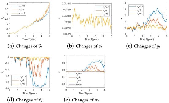 Figure A1. Illustrate the impact on (a) stock prices, (b) driver of volatility, (c) driver of elasticity, (d) elasticity of volatility, and (e) optimal stock allocations when varying the speed of reversion, .
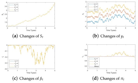 Figure A2. Illustrate the impact on (a) stock prices, (b) driver of elasticity, (c) elasticity of volatility, and (d) optimal stock allocations when varying .
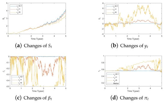 Figure A3. Illustrate the impact on (a) stock prices, (b) driver of elasticity, (c) elasticity of volatility, and (d) optimal stock allocations when varying .
 - Bear market conditions (Figure A4, Figure A5 and Figure A6):
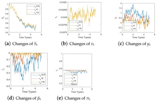 Figure A4. Illustrate the impact on (a) stock prices, (b) driver of volatility, (c) driver of elasticity, (d) elasticity of volatility, and (e) optimal stock allocations when varying the speed of reversion, .
 Figure A5. Illustrate the impact on (a) stock prices, (b) driver of elasticity, (c) elasticity of volatility, and (d) optimal stock allocations when varying θy(e.g., θy = −1, 0, 1).
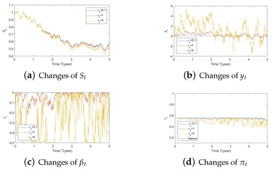 Figure A6. Illustrate the impact on (a) stock prices, (b) driver of elasticity, (c) elasticity of volatility, and (d) optimal stock allocations when varying .
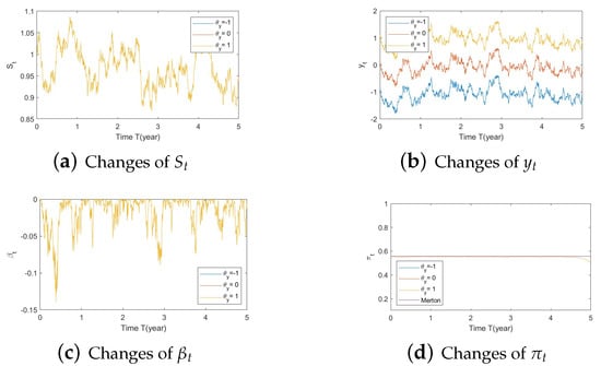
Figure A8.
Illustrate the impact on (a) stock prices, (b) driver of elasticity, (c) elasticity of volatility, and (d) optimal stock allocations when varying .
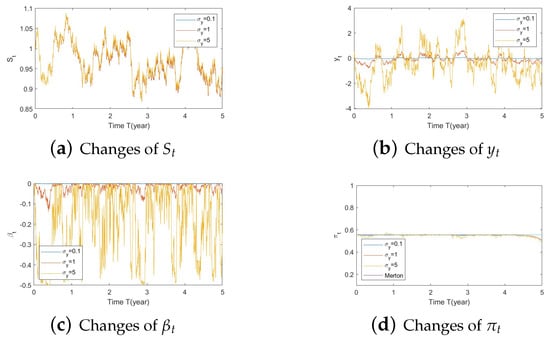
Figure A9.
Illustrate the impact on (a) stock prices, (b) driver of elasticity, (c) elasticity of volatility, and (d) optimal stock allocations when varying .
Appendix A.3.2. Figures of Arctan Function Analysis
- Bull market conditions (Figure A10, Figure A11 and Figure A12):
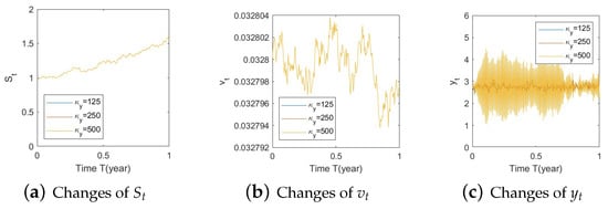
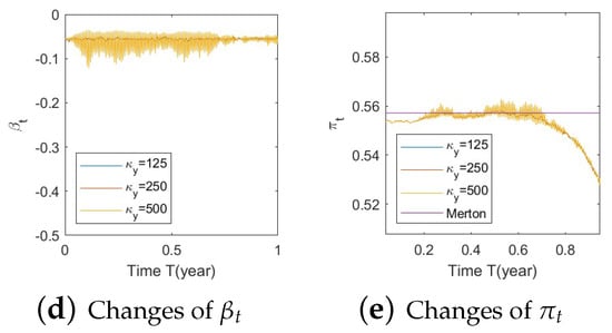 Figure A10. Illustrate the impact on (a) stock prices, (b) driver of volatility, (c) driver of elasticity, (d) elasticity of volatility, and (e) optimal stock allocations when varying the speed of reversion, .
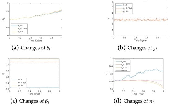 Figure A11. Illustrate the impact on (a) stock prices, (b) driver of elasticity, (c) elasticity of volatility, and (d) optimal stock allocations when varying θy(e.g., θy = −5, 2.7505, 15).
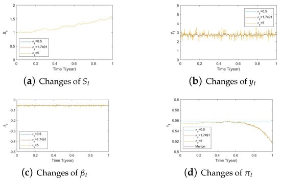 Figure A12. Illustrate the impact on (a) stock prices, (b) driver of elasticity, (c) elasticity of volatility, and (d) optimal stock allocations when varying .
 - Bear market conditions (Figure A13, Figure A14 and Figure A15):
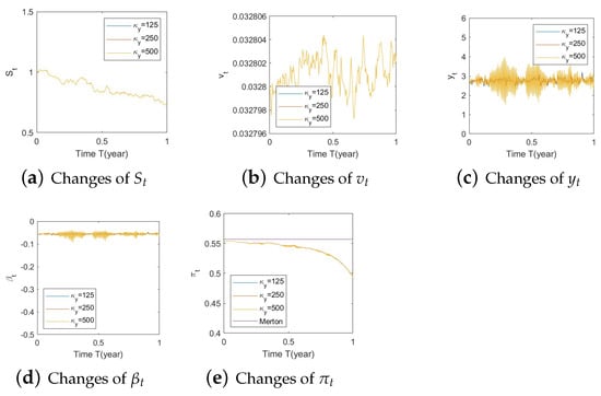 Figure A13. Illustrate the impact on (a) stock prices, (b) driver of volatility, (c) driver of elasticity, (d) elasticity of volatility, and (e) optimal stock allocations when varying the speed of reversion, .
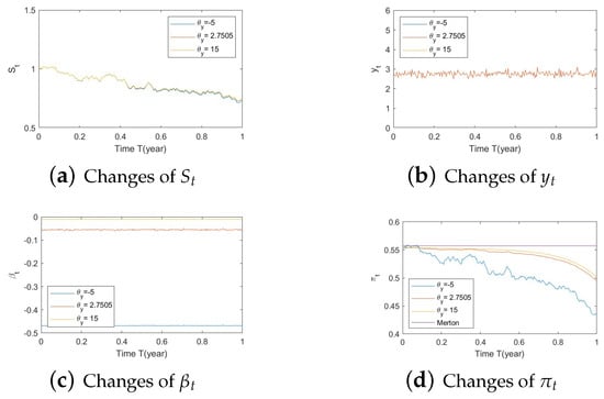 Figure A14. Illustrate the impact on (a) stock prices, (b) driver of elasticity, (c) elasticity of volatility, and (d) optimal stock allocations when varying .
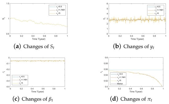 Figure A15. Illustrate the impact on (a) stock prices, (b) driver of elasticity, (c) elasticity of volatility, and (d) optimal stock allocations when varying .
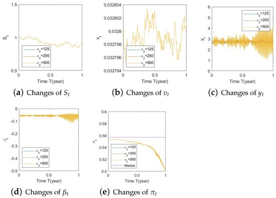
Figure A16.
Illustrate the impact on (a) stock prices, (b) driver of volatility, (c) driver of elasticity, (d) elasticity of volatility, and (e) optimal stock allocations when varying the speed of reversion, .
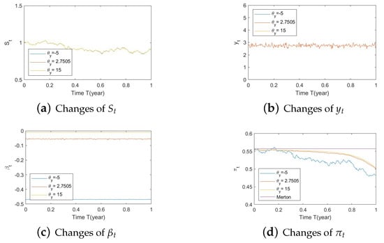
Figure A17.
Illustrate the impact on (a) stock prices, (b) driver of elasticity, (c) elasticity of volatility, and (d) optimal stock allocations when varying .


Figure A18.
Illustrate the impact on (a) stock prices, (b) driver of elasticity, (c) elasticity of volatility, and (d) optimal stock allocations when varying .
Appendix A.4. SEV Analysis
Appendix A.4.1. Figures of Gaussian Function Analysis
- 1.
- Bull market conditions (Figure A19, Figure A20 and Figure A21):
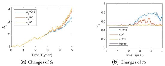 Figure A19. Illustrate the impact on (a) stock prices and (b) optimal stock allocations when varying the speed of reversion .
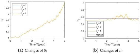 Figure A20. Illustrate the impact on (a) stock prices and (b) optimal stock allocations when varying θy(e.g., θy = −1, 0, 1).
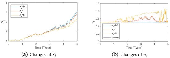 Figure A21. Illustrate the impact on (a) stock prices and (b) optimal stock allocations when varying .
 - 2.
- Bear market conditions (Figure A22, Figure A23 and Figure A24):
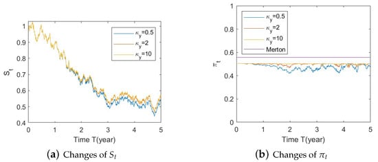 Figure A22. Illustrate the impact on (a) stock prices and (b) optimal stock allocations when varying the speed of reversion .
 Figure A23. Illustrate the impact on (a) stock prices and (b) optimal stock allocations when varying .
 Figure A24. Illustrate the impact on (a) stock prices and (b) optimal stock allocations when varying .
 - 3.
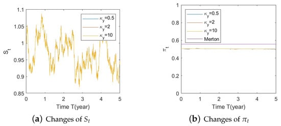
Figure A25.
Illustrate the impact on (a) stock prices and (b) optimal stock allocations when varying the speed of reversion .

Figure A26.
Illustrate the impact on (a) stock prices and (b) optimal stock allocations when varying .

Figure A27.
Illustrate the impact on (a) stock prices and (b) optimal stock allocations when varying .
Appendix A.4.2. Figures of Arctan Function Analysis
- 1.
- Bull market conditions (Figure A28, Figure A29 and Figure A30):
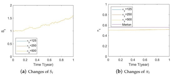 Figure A28. Illustrate the impact on (a) stock prices and (b) optimal stock allocations when varying the speed of reversion, .
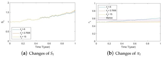 Figure A29. Illustrate the impact on (a) stock prices and (b) optimal stock allocations when varying .
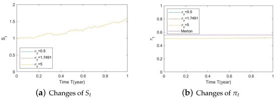 Figure A30. Illustrate the impact on (a) stock prices and (b) optimal stock allocations when varying .
 - 2.
- Bear market conditions (Figure A31, Figure A32 and Figure A33):
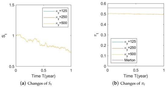 Figure A31. Illustrate the impact on (a) stock prices and (b) optimal stock allocations when varying the speed of reversion, .
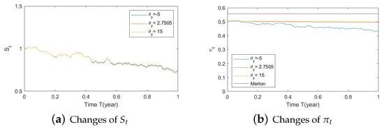 Figure A32. Illustrate the impact on (a) stock prices and (b) optimal stock allocations when varying .
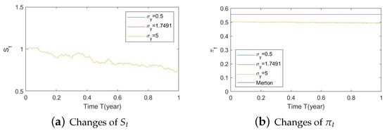 Figure A33. Illustrate the impact on (a) stock prices and (b) optimal stock allocations when varying .
 - 3.
- Normal market conditions (Figure A34, Figure A35 and Figure A36):
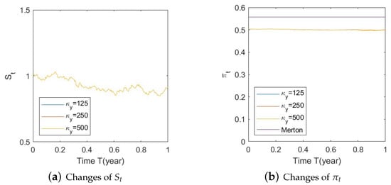 Figure A34. Illustrate the impact on (a) stock prices and (b) optimal stock allocations when varying the speed of reversion, .
 Figure A35. Illustrate the impact on (a) stock prices and (b) optimal stock allocations when varying .
 Figure A36. Illustrate the impact on (a) stock prices and (b) optimal stock allocations when varying .
Notes
| 1 | In principle, an incomplete market setting permits infinitely many risk-neutral measures, nonetheless investors can select one using options in an approach called market completion. |
| 2 | This provides necessary conditions. |
References
- Beckers, Stan. 1980. The constant elasticity of variance model and its implications for option pricing. The Journal of Finance 35: 661–73. [Google Scholar] [CrossRef]
- Boguslavskaya, Elena, and Dmitry Muravey. 2016. An explicit solution for optimal investment in heston model. Theory of Probability & Its Applications 60: 679–88. [Google Scholar]
- Cao, Jiling, Jeong-Hoon Kim, and Wenjun Zhang. 2021. Pricing variance swaps under hybrid cev and stochastic volatility. Journal of Computational and Applied Mathematics 386: 113220. [Google Scholar] [CrossRef]
- Chacko, George, and Luis M. Viceira. 2005. Dynamic consumption and portfolio choice with stochastic volatility in incomplete markets. The Review of Financial Studies 18: 1369–402. [Google Scholar] [CrossRef]
- Cheng, Yuyang, and Marcos Escobar-Anel. 2021. Optimal investment strategy in the family of 4/2 stochatic volatility models. Quantitative Finance 21: 1723–51. [Google Scholar] [CrossRef]
- Cheng, Yuyang, and Marcos Escobar-Anel. 2022. A class of portfolio optimization solvable problems. Finance Research Letters, 103373. [Google Scholar] [CrossRef]
- Choi, Sun-Yong, Jean-Pierre Fouque, and Jeong-Hoon Kim. 2013. Option pricing under hybrid stochastic and local volatility. Quantitative Finance 13: 1157–65. [Google Scholar] [CrossRef]
- Cox, John. 1975. Notes on Option Pricing I: Constant Elasticity of Variance Diffusions. Unpublished note, Stanford University, Graduate School of Business, Stanford, CA, USA. [Google Scholar]
- Cox, John C. 1996. The constant elasticity of variance option pricing model. Journal of Portfolio Management 23: 15–17. [Google Scholar] [CrossRef]
- Cox, John C., and Stephen A. Ross. 1976. The valuation of options for alternative stochastic processes. Journal of Financial Economics 3: 145–66. [Google Scholar]
- Cui, Zhenyu, J. Lars Kirkby, and Duy Nguyen. 2017a. Equity-linked annuity pricing with cliquet-style guarantees in regime-switching and stochastic volatility models with jumps. Insurance: Mathematics and Economics 74: 46–62. [Google Scholar]
- Cui, Zhenyu, J. Lars Kirkby, and Duy Nguyen. 2017b. A general framework for discretely sampled realized variance derivatives in stochastic volatility models with jumps. European Journal of Operational Research 262: 381–400. [Google Scholar] [CrossRef]
- Cui, Zhenyu, J. Lars Kirkby, and Duy Nguyen. 2018. A general valuation framework for sabr and stochastic local volatility models. SIAM Journal on Financial Mathematics 9: 520–63. [Google Scholar] [CrossRef]
- Davydov, Dmitry, and Vadim Linetsky. 2001. The valuation and hedging of barrier and lookback options under the cev process. Management Science 47: 949–65. [Google Scholar]
- Emanuel, David C., and James D. MacBeth. 1982. Further results on the constant elasticity of variance call option pricing model. Journal of Financial and Quantitative Analysis 17: 533–54. [Google Scholar] [CrossRef]
- Gao, Jianwei. 2009. Optimal portfolios for dc pension plans under a cev model. Insurance: Mathematics and Economics 44: 479–90. [Google Scholar]
- Gao, Jianwei. 2010. An extended cev model and the legendre transform–dual–asymptotic solutions for annuity contracts. Insurance: Mathematics and Economics 46: 511–30. [Google Scholar] [CrossRef]
- Ghysels, Eric, Andrew C. Harvey, and Eric Renault. 1996. 5 stochastic volatility. Handbook of Statistics 14: 119–91. [Google Scholar]
- Grasselli, Martino. 2017. The 4/2 stochastic volatility model: A unified approach for the heston and the 3/2 model. Mathematical Finance 27: 1013–34. [Google Scholar] [CrossRef]
- Harvey, Campbell R. 2001. The specification of conditional expectations. Journal of Empirical Finance 8: 573–637. [Google Scholar] [CrossRef]
- Heston, Steven L. 1993. A closed-form solution for options with stochastic volatility with applications to bond and currency options. The Review of Financial Studies 6: 327–43. [Google Scholar] [CrossRef]
- Heston, Steven L. 1997. A Simple New Formula for Options with Stochastic Volatility. St. Louis: Washington University in St. Louis. [Google Scholar]
- Kim, Jeong-Hoon, Jungwoo Lee, Song-Ping Zhu, and Seok-Hyon Yu. 2014. A multiscale correction to the black–scholes formula. Applied Stochastic Models in Business and Industry 36: 753–65. [Google Scholar]
- Kim, Jeong-Hoon, Ji-Hun Yoon, Jungwoo Lee, and Sun-Yong Choi. 2015. On the stochastic elasticity of variance diffusions. Economic Modelling 51: 263–68. [Google Scholar] [CrossRef]
- Kraft, Holger. 2005. Optimal portfolios and heston’s stochastic volatility model: An explicit solution for power utility. Quantitative Finance 5: 303–13. [Google Scholar] [CrossRef]
- Lions, P.-L., and Marek Musiela. 2007. Correlations and bounds for stochastic volatility models. Annales De L’Institut Henri Poincaré C, Analyse Non Linéaire 24: 1–16. [Google Scholar] [CrossRef]
- Lo, Chi Fai, P. H. Yuen, and Cho-Hoi Hui. 2000. Constant elasticity of variance option pricing model with time-dependent parameters. International Journal of Theoretical and Applied Finance 3: 661–74. [Google Scholar] [CrossRef]
- Lord, Roger, Remmert Koekkoek, and Dick Van Dijk. 2010. A comparison of biased simulation schemes for stochastic volatility models. Quantitative Finance 10: 177–194. [Google Scholar] [CrossRef]
- MacBeth, James D., and Larry J. Merville. 1980. Tests of the black-scholes and cox call option valuation models. The Journal of Finance 35: 285–301. [Google Scholar] [CrossRef]
- Merton, Robert C. 1969. Lifetime portfolio selection under uncertainty: The continuous-time case. The review of Economics and Statistics 51: 247–57. [Google Scholar] [CrossRef]
- Platen, E. 1997. A Non-Linear Stochastic Volatility Model. Financial Mathematics Research Report No. FMRR 005-97. Canberra: Center for Financial Mathematics, Australian National Universite. [Google Scholar]
- Yuen, K. C., H. Yang, and K. L. Chu. 2001. Estimation in the constant elasticity of variance model. British Actuarial Journal 7: 275–92. [Google Scholar] [CrossRef]
Disclaimer/Publisher’s Note: The statements, opinions and data contained in all publications are solely those of the individual author(s) and contributor(s) and not of MDPI and/or the editor(s). MDPI and/or the editor(s) disclaim responsibility for any injury to people or property resulting from any ideas, methods, instructions or products referred to in the content. |
© 2023 by the authors. Licensee MDPI, Basel, Switzerland. This article is an open access article distributed under the terms and conditions of the Creative Commons Attribution (CC BY) license (https://creativecommons.org/licenses/by/4.0/).
