Article

Analysing Quantiles in Models of Forward Term Rates

by
Thomas A. McWalter
1,2,
Erik Schlögl
1,2,3 and
Jacques van Appel
2,*
1
The African Institute of Financial Markets and Risk Management (AIFMRM), University of Cape Town, Cape Town 7701, South Africa
2
Faculty of Science, Department of Statistics, University of Johannesburg, Johannesburg 2006, South Africa
3
School of Mathematical and Physical Sciences, University of Technology Sydney, Ultimo, NSW 2007, Australia
*
Author to whom correspondence should be addressed.
Risks 2023, 11(2), 29; https://doi.org/10.3390/risks11020029
Submission received: 29 November 2022 / Revised: 12 January 2023 / Accepted: 13 January 2023 / Published: 28 January 2023

Abstract

:
The class of forward-LIBOR market models can, under certain volatility structures, produce unrealistically high long-dated forward rates, particularly for maturities and tenors beyond the liquid market calibration instruments. This paper presents a diagnostic tool for analysing the quantiles of distributions for forward term rates in a displaced lognormal forward-LIBOR model (DLFM). In particular, we provide a quantile approximation that can be used to assess whether the modelled term rates remain within realistic bounds with a high probability. Applying this diagnostic tool (verified using Quasi-Monte Carlo (QMC) simulations), we show that realised forward term rates for long time horizons may be kept within realistic limits by appropriately damping the tail of the DLFM volatility function.

1. Introduction

Early one-factor short rate models were able to keep long-dated interest rates within realistic limits by using a mean reversion feature (see, e.g., Vasiček 1977; Cox et al. 1985; or Hull and White 1990). Mean reverting short rates tend to decrease when high and increase when low. This property is imposed in the risk-neutral instantaneous short rate dynamics by a component of the drift dependent on the level of the short rate. However, if one considers the resulting dynamics of these models for, say, quarterly forward rates with simple compounding, when viewed under the respective forward measures to the end of their accrual periods, mean reversion manifests itself in the fact that the volatility of these rates decay with increasing time to maturity; there is no “mean reverting” component in the drift of these rates because simply compounded forward rates must be martingales (i.e., driftless) under the forward measure to the end of the accrual period in any arbitrage-free model.
Historically, simply compounded forward rates have had the label “forward LIBOR”, and models constructed directly on the basis of such market-quoted rates were called “LIBOR Market Models” (LMM).1 While the London Interbank Offer Rate (LIBOR) and similar interest rate benchmarks in other jurisdictions are widely2 being replaced by benchmarks based on overnight rates, such as the Secured Overnight Funding Rate (SOFR) in the United States, simply compounded term rates are still key market objects. Consequently, the LMM and its extensions remain important tools for the modelling of interest rate risks.3 In keeping with long-standing convention, we shall speak of simply compounded forward rates as “forward LIBORs.”
In such models, a decay of forward rate volatility with increasing time to maturity must be introduced explicitly (as opposed to implicitly via the mean reversion feature in short rate models) in order to prevent unrealistic long-term behaviour of the model dynamics. This is also true of models specified in terms of the volatilities of instantaneous forward rates in the Heath et al. (1992) (HJM) framework; however, in the present paper, we focus on models specified in terms of volatilities of simply compounded forward rates, i.e., LMM-type models.4 When choosing a volatility specification, there is no readily available algorithm to determine whether the choice will lead to realistically bounded realised forward LIBORs, other than using time-consuming Monte-Carlo methods. This is particularly important when extrapolating beyond the reach of current market calibration instruments when, for example, modelling the risk of longer-dated liabilities.5 In this paper, we develop and show the efficacy of a diagnostic tool for analysing the distributional behaviour of realised forward LIBORs arising from volatility specifications. This is useful for detecting poorly performing volatility parametrisations and evaluating the effectiveness of mitigation strategies.
We focus on a displaced diffusion extension of the LMM, namely the displaced lognormal forward-LIBOR model (DLFM), since it is more flexible (discussed in Section 2 below) yet still analytically tractable. In particular, we provide an efficient quantile approximation using the moment approximations derived in Van Appel and McWalter (2018, 2020), which are adapted here to the more generally applicable spot risk-neutral measure.6 Quasi-Monte Carlo (QMC) simulations show that our quantile approximation is an accurate and useful tool in analysing the distributional behaviour of long-dated forward-LIBOR rates. We then show that unrealistically high forward-LIBOR rates may be kept within realistic limits by appropriately damping the long-dated background volatility tail using, for example, a sigmoid function.
The paper is structured as follows. Section 2 describes some requirements of a modern term structure model and provides an overview of the DLFM under the spot risk-neutral measure. Section 3 introduces our quantile approximation with an outline of the Van Appel and McWalter (2020) moment approximation algorithm adapted to the spot measure. The accuracy of our quantile approximation is demonstrated under different scenarios in Section 4 using QMC simulations. Furthermore, we describe a useful volatility damping methodology to keep long-dated forward-LIBOR rates within realistic limits. We conclude with Section 5.

2. The Model

Complex derivatives have highlighted the need for term structure models that can produce changes in the shape, both in the gradient and curvature, of the yield curve. A model may gain this ability through the mechanisms of time-dependent volatilities or multiple driving factors. The latter allows financially convincing instantaneous forward rate correlation structures while the former is just as financially sound and capable of producing the desired terminal de-correlation, even in a one-factor model (see, e.g., Fries 2007, sct. 21.2.1). We do not consider the effectiveness of either mechanism individually since the class of forward-LIBOR market models inherently possesses both.
Our focus is on the DLFM, firstly, for its ability to capture skew effects and remain analytically tractable. Secondly, it can produce CEV-like skews with a parsimonious parametrisation (see, e.g., chp. 3 of Brace 2008 or Svoboda-Greenwood 2009). Furthermore, under a specific parameter specification, the DLFM may describe any discretized Gaussian model within the HJM framework (see, e.g., chp. 24 of Fries 2007; chp. 3 of Brace 2008; or chp. 14 of Andersen and Piterbarg 2010b). This is accomplished by setting the DLFM displacement parameter equal to the reciprocal of the accrual period of each rate, integrating the instantaneous forward rate volatility function over the discrete forward LIBOR tenors, and specifying the appropriate correlation structure. Lastly, the DLFM can produce negative forward LIBORs under a suitable parametrisation, which has become a desirable feature in periods of extremely low interest rates.
An important modelling consideration is the pricing measure. We may choose between the T-forward, terminal or spot measures. The latter is induced by a discretely compounded analog of the continuously compounded bank account numéraire, while the terminal measure corresponds to a special case of the T-forward measure in which the numéraire is the last modelled maturity zero-coupon bond. The terminal and spot measures are suitable when it comes to derivatives that require a numéraire that remains alive over the entire tenor structure. We, however, prefer the spot measure since it can be extended to any time horizon by simple compounding and it is more efficient when it comes to simulation. More specifically, under the terminal measure very large forward LIBOR realizations produce very small zero-coupon bond prices, resulting in normalized payoffs becoming very large (see, e.g., Example 5.1 in Brace 2008).
To fix notation, definitions, and terminology used throughout the paper, let tenor dates be given by 0 = : T 0 < T 1 < < T M < T M + 1 . The time-t price of a zero-coupon bond paying a unit of currency at maturity T i is denoted P ( t , T i ) . Define the accrual factors as τ i = T i + 1 T i , in which case the time-t value of the forward LIBOR from T i to T i + 1 is given by
F i ( t ) : = F t ; T i , T i + 1 = 1 τ i P t , T i P t , T i + 1 1 .
We denote by Q B the spot measure associated with the numéraire asset7
B ( t ) : = P t , T ϑ ( t ) i = 0 ϑ ( t ) 1 1 + τ i F i ( T i ) ,
where ϑ ( t ) : = min { i : T i t } . Then the DLFM dynamics of F i ( t ) under Q B are
d F i ( t ) = μ ˜ i ( t ) ( F i ( t ) + a i ) d t + σ i ( t ) ( F i ( t ) + a i ) d W i B ( t ) ,
for t T i , where
μ ˜ i ( t ) : = σ i ( t ) j = ϑ ( t ) i ρ i j σ j ( t ) τ j ( F j ( t ) + a j ) 1 + τ j F j ( t ) ,
a i are the constant displacement factors, σ i ( t ) is the instantaneous volatility of F i ( t ) , and W i B ( t ) is the ith component of an M-dimensional Q B Brownian motion with instantaneous correlations given by:
d W i B , W j B t = ρ i j d t .
The correlation matrix formed by the elements ρ i j is denoted by ρ and is assumed to be of rank n. If n = M , then ρ is full rank.
It is worth remarking that the forward rates in (3) have an unknown distribution but are approximately displaced-lognormally distributed, and as a consequence, F i ( t ) + a i are approximately lognormally distributed. Under the assumption of lognormality of F i ( t ) + a i , Van Appel and McWalter (2020) derive a computationally tractable algorithm that accurately and efficiently approximates the moments of the forward rate distribution under the T-forward measure. In the next section, we adapt this algorithm to the spot measure and provide a quantile approximation.

3. Quantile Approximation

In this section, we provide an algorithm for a computationally tractable quantile approximation of the entire forward rate curve under the spot measure, Q B . We closely follow the terminology and notation set out in Van Appel and McWalter (2020) by defining a vector of displaced forward rates, H ( t ) , in terms of vectors F ( t ) and a with the elements F i ( t ) and a i , for 1 i M and t T i , as
H ( t ) : = F ( t ) + a .
Let H ¯ ( t ) and Σ H ( t ) denote the mean and covariance of H ( t ) . Then, we assume that
Y ( t ) : = log H ( t )
is normally distributed as
Y ( t ) N Y ¯ ( t ) , Σ Y ( t ) ,
where Y ¯ ( t ) and Σ Y ( t ) are the mean and covariance, respectively, so that H ( t ) is lognormally distributed as
H ( t ) log N Y ¯ ( t ) , Σ Y ( t ) .
Therefore, the quantile of each realised forward rate, F i ( T i ) , for 1 i M is
Q i F p ; Y ¯ i ( T i ) , Σ i i Y ( T i ) = exp Y ¯ i ( T i ) + 2 Σ i i Y ( T i ) erf 1 ( 2 p 1 ) a i ,
where
p : = Q B F i ( T i ) < Q i F p ; Y ¯ i ( T i ) , Σ i i Y ( T i )
with Y ¯ i ( T i ) and Σ i j Y ( T i ) determined recursively through time in increments of Δ . We outline this algorithm in the following steps:
  • For T ϑ ( t ) 1 t < T ϑ ( t ) and ϑ ( t ) { i , j } M , calculate
    Y ¯ i ( t ) = log H ¯ i ( t ) 1 2 Σ i i Y ( t )
    and
    Σ i j Y ( t ) = log Σ i j H ( t ) H ¯ i ( t ) H ¯ j ( t ) + 1 ,
    where H ¯ ( 0 ) = H ( 0 ) , Y ¯ ( 0 ) = Y ( 0 ) and Σ H ( 0 ) = Σ Y ( 0 ) = 0 .
  • Determine
    Y ¯ i ( t + Δ ) = U i ( X ¯ ) + 1 2 tr 2 U i ( X ¯ ) Σ X
    and
    Σ i j Y ( t + Δ ) = U i ( X ¯ ) Σ X U j ( X ¯ ) + 1 2 tr Σ X 2 U i ( X ¯ ) Σ X 2 U j ( X ¯ )
    for ϑ ( t ) { i , j } M , where tr ( · ) is the trace operator using
    U i ( X ) : = [ Y i ( t ) + μ i ( t ) Δ + 1 2 L 0 μ i ( t ) Δ 2 + h = 1 n σ i ( t ) ρ ˜ i h Δ B h + L h μ i ( t ) Δ B ˜ h ] X
    with
    μ i ( t ) = σ i ( t ) j = ϑ ( t ) i ρ i j σ j ( t ) τ j ( F j ( t ) + a j ) 1 + τ j F j ( t ) 1 2 σ i 2 ( t ) ,
    and where L 0 μ i ( t ) and L h μ i ( t ) are defined in (A1) and (A2), respectively. The random variable
    X : = [ Y ( t ) , B ]
    is composed of two independent multivariate normal random variables, Y ( t ) and B N 0 , Σ B , where
    B : = Δ B 1 Δ B ˜ 1 Δ B 2 Δ B ˜ 2 Δ B n Δ B ˜ n and Σ B : = Δ 1 2 Δ 2 0 0 0 0 1 2 Δ 2 1 3 Δ 3 0 0 0 0 0 0 Δ 1 2 Δ 2 0 0 0 0 1 2 Δ 2 1 3 Δ 3 0 0 0 0 0 0 Δ 1 2 Δ 2 0 0 0 0 1 2 Δ 2 1 3 Δ 3 .
    Thus, X N X ¯ , Σ X with
    X ¯ = Y ¯ ( t ) 0 and Σ X = Σ Y ( t ) 0 0 Σ B .
    The elements of the gradient, U i ( X ¯ ) , Hessian, 2 U i ( X ¯ ) , and their corresponding derivatives can be found in Appendix A.2. It is worth remarking that since (10) only requires the diagonal elements of Σ Y we may significantly reduce the execution time by computing
    Σ i i Y ( t + Δ ) = U i ( X ¯ ) Σ X U i ( X ¯ ) + 1 2 tr Σ X 2 U i ( X ¯ ) Σ X 2 U i ( X ¯ )
    and using
    Σ i j Y ( t + Δ ) Σ i i Y ( t + Δ ) ρ i j Σ j j Y ( t + Δ )
    to approximate the off-diagonal elements. The resulting trade-off, along with a lower-order approximation, is fully explored in Van Appel and McWalter (2020).
  • Compute
    H ¯ i ( t + Δ ) = exp Y ¯ i ( t + Δ ) + 1 2 Σ i i Y ( t + Δ )
    and
    Σ i j H ( t + Δ ) = H ¯ i ( t + Δ ) H ¯ j ( t + Δ ) exp Σ i j Y ( t + Δ ) 1 .
  • If t + Δ < T M , repeat steps 1 through to 3.
  • Once all the rates are evolved to expiry, the quantiles Q i F p ; Y ¯ i ( T i ) , Σ i i Y ( T i ) are computed using (10) for each F i and T i , with 1 i M .
In the following section, we demonstrate the capability of the quantile approximation in (10) as a diagnostic tool to analyse the long-dated behaviour of forward LIBORs implied by the model.

4. Numerical Results

To verify the capability of the quantile approximation, given in (10), we used QMC simulations. In particular, we use Sobol’ sequences (see Joe and Kuo (2003, 2008)), Brownian-bridging and a predictor-corrector algorithm (see Hunter et al. 2001), in conjunction with 2 20 1 sample paths of F i ( t ) , for 1 i M = 199 and τ i = 0.25 , at times t { 0 , Δ , 2 Δ , , T i } with increments of Δ = 0.25 . Furthermore, to allow the replication of our results, we used the flexible and well-known instantaneous volatility parametrisation
σ i ( t ) : = σ ( t , T i , a , b , c , d ) = a + b T i t e c ( T i t ) + d ,
while making the piecewise constant assumption
σ i j 2 : = 1 τ j T j T j + 1 σ i 2 ( t ) d t ,
for j = 0 , 1 , , α 1 .
The next subsection takes advantage of the fact that a special DLFM specification yields a discretized Gaussian model from within the HJM framework. This allows us to demonstrate the forward rate quantile, provided in (10), for well-behaved forward LIBORs under a mean reverting Gaussian short rate process described in the HJM framework. This example further illustrates the forward rate mechanism that keeps long-dated forward rates bounded and realistic.

4.1. DLFM Specification of a Discretized HJM Model

The model in this section is for illustrative purposes. For its simplicity, we considered a one-factor mean-reverting Vasiček model, which has an initial instantaneous forward rate curve that is given by
f ( 0 , T ) = μ V + e α V T r ( 0 ) μ V σ V 2 2 α V 2 1 e α V T 2 ,
where r denotes the instantaneous short rate. The model parameters { α V , μ V , σ V } and r ( 0 ) are positive constants with their classical interpretation; that is, r ( 0 ) is the initial short rate or spot rate, α V is the mean reversion speed, μ V is the long-run mean of the process and σ V is the short rate volatility. Then, in the terms of the HJM framework, the Vasiček model evolves the instantaneous forward rate according to
d f ( t , T ) = σ f ( t , T ) t T σ f ( t , s ) d s d t + σ f ( t , T ) d B Q ( t ) ,
where B Q is a standard Brownian motion under the risk-neutral measure, which is associated with the usual bank account numéraire and
σ f ( t , T ) = σ V exp α V ( T t )
is the instantaneous forward rate volatility.
The volatility function in (27) provides a key insight for forward rates derived from a mean-reverting short rate process; the time-homogeneous forward rate volatility structure must exponentially decay to zero with increasing time to maturity.
The above HJM model description can be discretized to yield a DLFM using a particular specification as follows (for details on linking the HJM and DLFM, see, e.g., chp. 24 of Fries 2007; chp. 3 of Brace 2008; or chp. 14 of Andersen and Piterbarg 2010b). For 1 i M , set the displacement parameter equal to the reciprocal of the accrual period,
α i = 1 τ i ,
and construct the discrete tenor volatility by integrating the instantaneous forward rate volatility in (27) over the LIBOR tenor structure to produce
σ i ( t ) : = T i T i + 1 σ f ( t , s ) d s = σ t , T i , σ V α V 1 exp ( α V τ i ) , 0 , α V , 0 ,
which is a simple reformulation of (23). Then, determine the initial forward LIBOR curve, F i ( 0 ) , with the relationship in (1) using (25) to compute
P ( 0 , T i ) = exp 0 T i f ( 0 , s ) d s = exp V 1 ( 0 , T i ) V 2 ( 0 , T i ) r ( 0 ) ,
where
V 1 ( 0 , T i ) = V 2 ( 0 , T i ) T i μ V σ V 2 2 α V 2 σ V 2 4 α V V 2 ( 0 , T i ) 2
and
V 2 ( 0 , T i ) = 1 α V 1 exp ( α V T i ) .
To present this Vasiček example of well behaved realised long-dated forward LIBORs, we used the following model input parameters: α V = 0.15 , μ V = 0.09 , σ V = 0.025 , and r ( 0 ) = 0.07 . Figure 1a shows the Vasiček realised forward LIBOR standard deviation, denoted as Σ i i F ( T i ) : = Σ i i H ( T i ) , for 1 i M computed using (22) (red dots).8 Here, the rate of increase in the forward rate standard deviation decreases and flattens out for longer maturities. This is a direct result of the time-homogeneous forward rate volatility, which exponentially decays to zero with increasing time to maturity. This can be seen in Figure 2a, which is a visualisation of the integrated instantaneous Vasiček forward rate volatility, (27), given in (29). For 1 i M , Figure 1b shows the realised Vasiček forward LIBOR quantile, Q i F p ; Y ¯ i ( T i ) , Σ i i Y ( T i ) , given in (10), for p = { 0.01 , 0.5 , 0.99 } along with the mean, F ¯ i ( T i ) = H ¯ i ( T i ) α i , computed using (21). The p = { 0.01 , 0.99 } quantiles flatten out with increasing time to maturity, showing that the realised forward LIBORs remain bounded. Again, this is due to the time-homogeneous forward rate volatility, which exponentially decays to zero with increasing time to maturity, which prevents the forward rate process from diffusing when it is far from maturity. This effect can be seen in Figure 2b, which displays 2 6 1 sample path realisations of F i ( t ) for t T i with a fixed i = M = 199 . Figure 1 shows that our diagnostic tool is accurate when compared to the QMC sample estimates (black circles), which we take to be our benchmark, given the relatively large sample size along with the use of Brownian bridging and a predictor-corrector algorithm.
Given that we have demonstrated the link between well behaved realised forward LIBORs and a decaying volatility function, σ f ( t , T ) , under a simple scenario, we next explore the accuracy of our diagnostic tool in a more sophisticated multifactor scenario.

4.2. DLFM with a Background Level of Volatility

We consider an n = 5 factor DLFM scenario with input parameters taken from Van Appel and McWalter (2020). The initial forward-LIBOR rate curve is specified as:
F i ( 0 ) = log T i + 1 y + x , for F 0 ( 0 ) = 0.08 and F M ( 0 ) = 0.04
and ρ is the correlation matrix, which is the rank-n reduced version of the Schoenmakers and Coffey (2003) formulation, ρ SC , with elements specified by
ρ i j SC = exp | i j | M 1 log ρ + ζ M i j + 1 M 2 ,
where, 0 ζ log ρ and { i , j } M are tenor indices. The rank reduction method used is the approach of zeroing the smallest M n eigenvalues and rescaling (see, e.g., Brigo and Mercurio 2006, sct. 6.9.2). For the displacement factors, we chose the following CEV-inspired parametrisation (see, e.g., chp. 3 of Brace 2008 or Svoboda-Greenwood 2009):
a i = 1 γ γ F i ( 0 ) ,
where γ = 0.45 is the CEV elasticity parameter since it is parsimonious and produces CEV-like skews. Table 1 provides a summary of the DLFM volatility and correlation input parameters for this scenario.
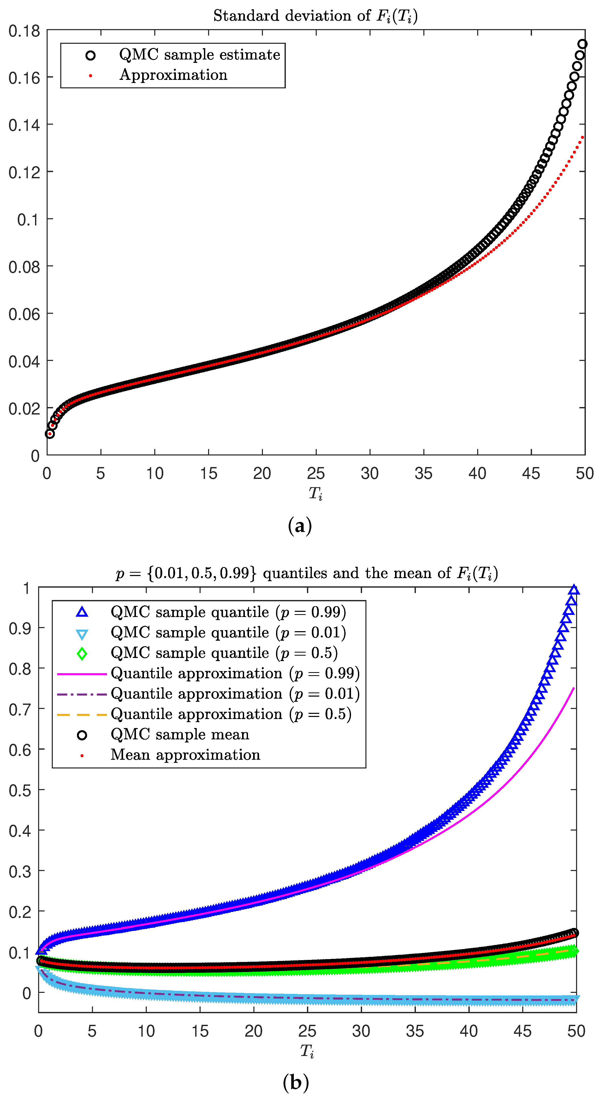
Here the realised forward LIBOR standard deviation does not flatten as in the Vasiček illustration of Section 4.1, but rather continues to increase with an upward curvature for long-dated maturities (as seen by comparing Figure 3a to Figure 1a). This is as a result of the level-d background volatility present in (23), which is responsible for diffusion of the long-term forward rates even when they are far from maturity. Figure 3b shows that this parameter set could be considered realistic for maturities out to approximately 35 years, with a p = 0.99 quantile of around 40%. For longer maturities, however, there is a clear upward curvature developing in the p = 0.99 realised forward LIBOR quantile (as with the realised forward LIBOR standard deviation in Figure 3a), which is an indication that forward LIBORs with longer maturities may encounter extreme outlier realisations. Further support for this is evident in the divergence between the mean and median realised forward LIBOR for the long maturities, which indicates that the large (outlier) sample paths become prominent. Exploding forward rates are well documented in the literature (see, e.g., Andersen and Piterbarg 2010a, sct. 4.5.3), with one solution being to restrict the volatility. This is the subject of the next section.
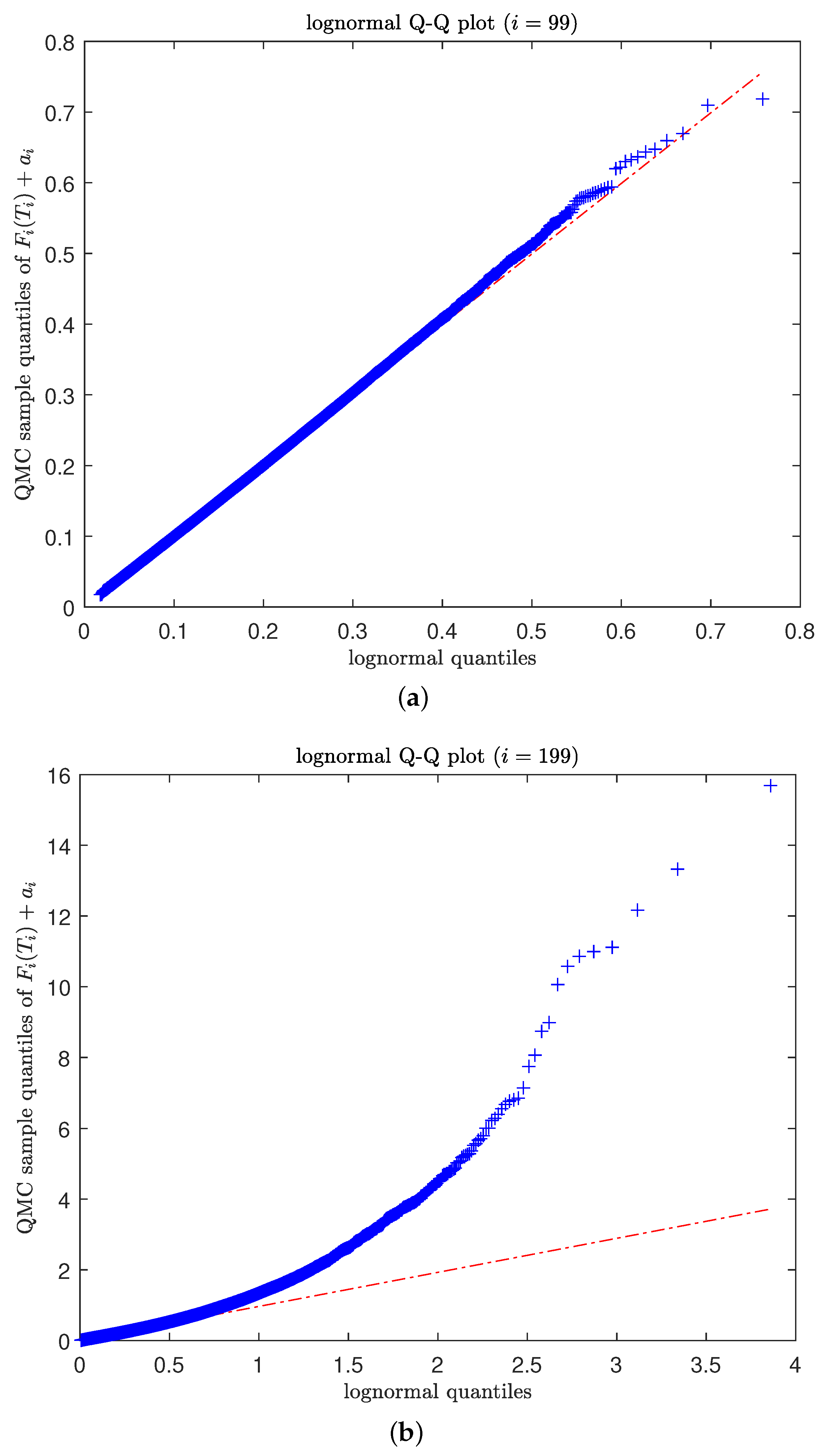
Figure 3 indicates that the approximations made by our diagnostic tool start to become less accurate for maturities longer than 35 years. This is seen in Figure 3a by comparing the realised forward rate standard deviation approximation, Σ i i F ( T i ) , (red dots) to the benchmark QMC sample estimates (black circles). A similar observation can be made in Figure 3b for the quantile approximation, Q i F 0.99 ; Y ¯ i ( T i ) , Σ i i Y ( T i ) , (magenta line). This is due to the gradual breakdown of the lognormal forward-LIBOR rate approximation, which can be seen in Figure 4, with the lognormal Q–Q plots for two different maturities. In particular, Figure 4a is a lognormal Q–Q plot of the realised sample QMC forward-LIBOR rate maturing at 25 years ( i = 99 ); here, the assumption of approximately lognormal forward-LIBOR rates is reasonable. However, the lognormal Q–Q plot in Figure 4b for the realised sample QMC forward rate maturing at 50 years ( i = M = 199 ) shows that the lognormal assumption erodes as a result of large outlier forward LIBOR realisations.
While the diagnostic tool in Figure 3 shows a loss of accuracy for long-dated forward LIBORs, this only occurs when the realised rates were already unrealistically high (greater than 50%). Thus, the quantile approximation is fit for the purpose of identifying unrealistically high rates, which only occur when the lognormal assumption breaks down. The next section describes a volatility-damping methodology that keeps long-dated forward LIBORs within realistic limits.

4.3. DLFM with Damped Background Volatility

We now demonstrate an approach that could be used to ensure realistic behaviour in the DLFM. This entails damping the level-d background volatility in (23) after a set cut-off time, T ˜ , using a sigmoid function with damping intensity, θ , defined as
σ ˜ i ( t ) = σ i ( t ) ς i ( t ) ,
where
ς i ( t ) : = 1 + I T i t > T ˜ erf 2 θ T i t T ˜ erf ( 2 ) 2 .
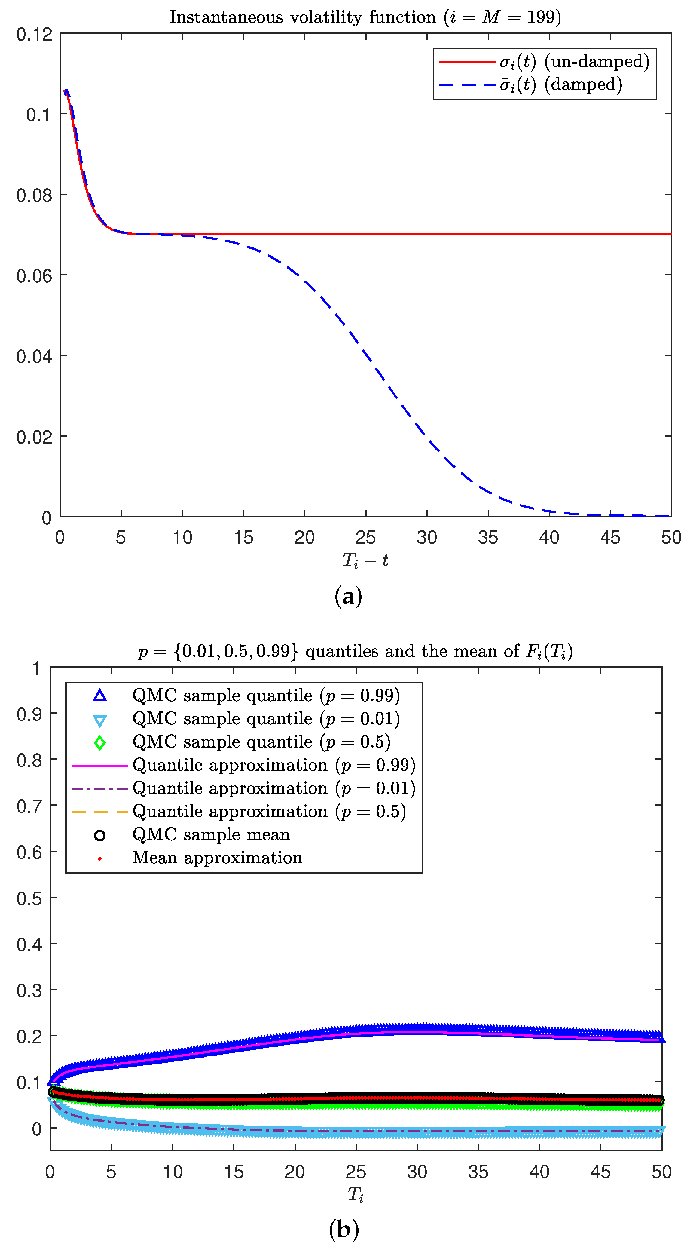
For illustration purposes, we set T ˜ = 8 years and θ = 0.11 . Figure 5a compares the un-damped volatility in (23), which includes the level-d background (red line), to the damped volatility in (36) (blue dashed line).
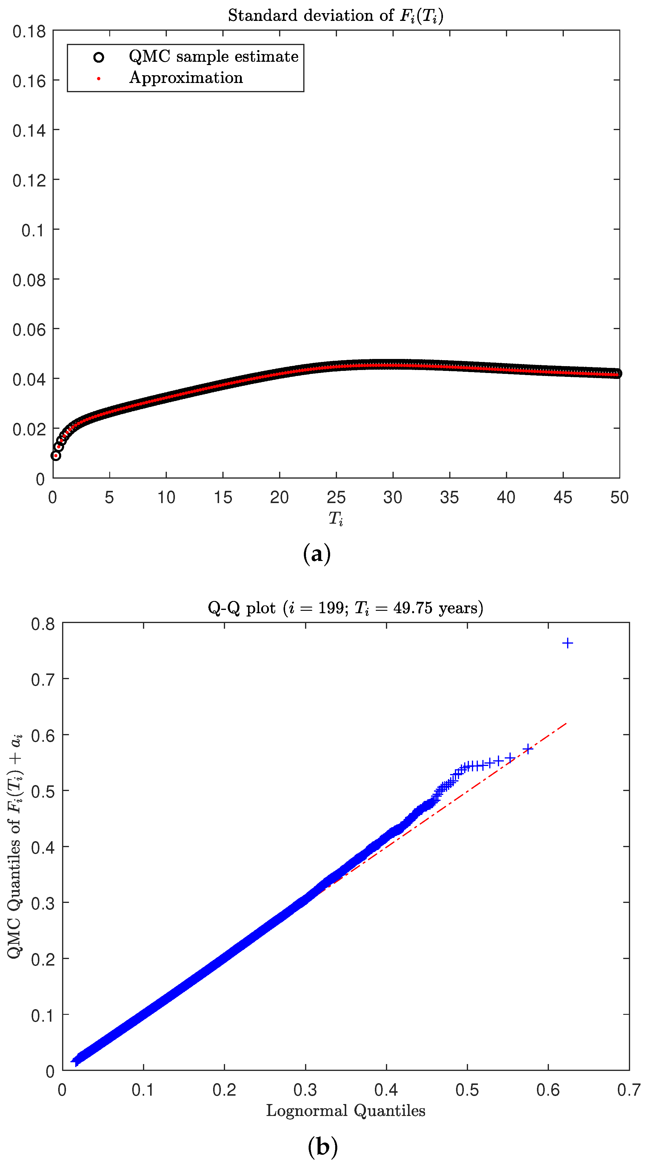
Using the damped instantaneous volatility function in (36), we reproduce the results from the DLFM scenario presented in Section 4.2. Firstly, by comparing Figure 5b and Figure 3b (which are generated on the same scale), it is clear that the damping of the instantaneous forward rate volatility has kept the long-dated realised forward LIBOR quantiles more tightly bound and realistic to the 50-year maturity. The realised forward LIBOR standard deviation in Figure 6a flattens out for longer maturities and does not continue to increase with an upward curvature as in Figure 3a. These results are reminiscent of those in Section 4.1 for the Vasiček illustration, with a similar bounding effect in the realised forward LIBOR quantiles and standard deviation. Finally, Figure 6b is a lognormal Q–Q plot of the sample QMC realised forward rate maturing at 50 years ( i = M = 199 ) and shows that the assumption of approximately lognormal forward LIBORs is now more plausible when compared to Figure 4b.
In summary, the parametrisation in (23) may provide flexibility while calibrating to the short end of the market with a background level, d, of volatility. However, this may lead to unrealistic outlier rate realisations for longer maturities and tenors, particularly those beyond the reach of current calibration instruments. In such cases, the quantile approximation, given in (10), may be used to identify if a given calibration produces realistic behaviour in the long-dated forward LIBORs.

5. Conclusions

The diagnostic tool presented in this paper allows for a tractable analysis of the distribution of long-dated forward term rates implied by the DLFM under different forward rate volatility parametrisations. This is particularly relevant for long-term asset/liability management (needed, for example, in the pension and life insurance industry), where one needs to model interest rates for maturities and tenors beyond the reach of current market calibration instruments. When poor-performing volatility specifications are detected, we have demonstrated that damping the instantaneous volatility function ameliorates the situation.
Migrating the forward LIBOR moment approximation approach of Van Appel and McWalter (2020) to the spot risk-neutral measure has the advantage of better numerical stability, and it also means that it is immediately clear that any reasonable market price of interest rate risk results in a negligible impact of carrying out the analysis under a risk-neutral rather than the statistical (a.k.a. “real-world”) measure. The change in drift between these two distributions is given by the market price of risk only (rather than being conflated with the volatility of some numéraire asset), and since we are only interested in quantiles of unrealistically high interest rates, this change in drift has a negligible effect on the outcome of the analysis using our tool.
QMC simulations show that our approach yields accurate quantiles when compared to benchmark estimates under realistic volatility specifications. When a volatility specification leads to a violation of the lognormal assumption, our method is less accurate. Even though accuracy is somewhat diminished in these cases, our quantile approximation remains viable for identifying unrealistic LIBOR ranges. In conclusion, our quantile approximation may be used to verify whether or not a DLFM calibration produces realistic behaviour.
Our approach of ensuring the realistic long-term behaviour of forward term rates is particularly useful for scenario generation in the pension and insurance industries, where claims must be priced beyond liquid market instruments. For example, the European Insurance and Occupational Pensions Authority (see EIOPA 2022) mandates that participants price claims beyond the last liquid point (LLP) in market rates. They require that the forward rate term structure is extrapolated to a constant ultimate forward rate (UFR), which is stipulated by regulation at regular intervals. This may well lead to the need to further dampen the modelled volatility of long-term forward rates;9 our tool can assist in implementing this in a realistic fashion. We anticipate conducting further research in this area by applying our approach under both the risk-neutral measure for pricing claims and the real-world measure for risk management.

Author Contributions

Conceptualisation, T.A.M., E.S. and J.v.A.; Formal analysis, T.A.M. and J.v.A.; Investigation, T.A.M., E.S. and J.v.A.; Methodology, T.A.M. and J.v.A.; Software, T.A.M. and J.v.A.; Supervision, T.A.M.; Visualisation, J.v.A.; Writing—original draft, T.A.M. and J.v.A.; Writing—review and editing, T.A.M., E.S. and J.v.A. All authors have read and agreed to the published version of the manuscript.

Funding

This research received no external funding.

Institutional Review Board Statement

Not applicable.

Informed Consent Statement

Not applicable.

Data Availability Statement

Not applicable.

Acknowledgments

The authors thank AIFMRM and David Taylor for providing us with access to the Intel Xeon server.

Conflicts of Interest

The authors declare no conflict of interest.

Appendix A. Expressions Needed in Section 3

Appendix A.1. Operators and Derivatives of U i ( X ¯ )

Suppressing t-dependence for brevity, the operators are given by
L 0 μ i = g = ϑ ( t ) i μ g μ i Y g + 1 2 σ g 2 2 μ i Y g 2 ,
L h μ i = g = ϑ ( t ) i σ g ρ ˜ g h μ i Y g ,
where the derivatives are10
μ i Y j = c i j x j , 2 μ i Y j 2 = c i j y j , 3 μ i Y j 3 = y j 2 μ i Y j 2 2 τ j c i j x j 2 , 4 μ i Y j 4 = y j 3 μ i Y j 3 6 τ j x j 2 μ i Y j 2 ,
for ϑ ( t ) i and k j in terms of
c i j = σ i ρ i j σ j τ j ( 1 a j τ j ) , x j = exp ( Y j ) ( 1 + τ j ( exp ( Y j ) a j ) ) 2 , y j = 1 τ j ( exp ( Y j ) + a j ) 1 + τ j ( exp ( Y j ) a j ) .

Appendix A.2. Gradient and Hessian Elements of U i ( X ¯ )

As in Appendix A.1 we suppress t dependence. The elements of the gradient, U i ( X ¯ ) , are
U i ( X ¯ ) Y i = μ i Y i Δ + 1 2 L 0 μ i Y i Δ 2 Y = Y ¯ + 1 , U i ( X ¯ ) Y j = μ i Y j Δ + 1 2 L 0 μ i Y j Δ 2 Y = Y ¯ for ϑ ( t ) j < i , U i ( X ¯ ) Δ B l = σ i ρ ˜ i l for 1 l n , U i ( X ¯ ) Δ B ˜ l = L l μ i | Y = Y ¯ for 1 l n ,
and the elements of the Hessian, 2 U i ( X ¯ ) , are
2 U i ( X ¯ ) Y j 2 = 2 μ i Y j 2 Δ + 1 2 2 L 0 μ i Y j 2 Δ 2 Y = Y ¯ for ϑ ( t ) j i , 2 U i ( X ¯ ) Y j Y k = 1 2 2 L 0 μ i Y j Y k Δ 2 | Y = Y ¯ for ϑ ( t ) { j , k } i and k j , 2 U i ( X ¯ ) Y j Δ B ˜ l = 2 U i ( X ¯ ) Δ B ˜ l Y j = L l μ i Y j | Y j = Y ¯ j for ϑ ( t ) j i and 1 l n ,
with all other elements in the Hessian equal to zero.11 In the above, the derivatives required are as follows:
L 0 μ i Y j = g = ϑ ( t ) i μ g Y j μ i Y g + μ j 2 μ i Y j 2 + 1 2 σ j 2 3 μ i Y j 3 , L h μ i Y j = σ j ρ ˜ j h 2 μ i Y j 2 , 2 L 0 μ i Y j 2 = g = ϑ ( t ) i μ i Y g 2 μ g Y j 2 + 2 μ j Y j 2 μ i Y j 2 + μ j 3 μ i Y j 3 + 1 2 σ j 2 4 μ i Y j 4 , 2 L 0 μ i Y j Y k = μ k Y j 2 μ i Y k 2 + μ j Y k 2 μ i Y j 2 ,
for ϑ ( t ) { j , k } i and k j , where the derivatives on the left of each equation are given in Appendix A.1.

Notes

1
Models of this type were first constructed by Miltersen et al. (1997); Musiela and Rutkowski (1997); Brace et al. (1997), and Jamshidian (1997).
2
But not everywhere: In the Eurozone, there are currently no plans to discontinue EURIBOR, and in Australia, the Australian version of this rate, the Bank Bill Swap Rate (BBSW), also remains in place.
3
In fact, there is considerable effort underway to adapt LMM-like models for markets based on overnight benchmarks, for example, Lyashenko and Mercurio (2019).
4
LMM-type models can also (often rather tediously) be expressed in the HJM framework, see e.g., Miltersen et al. (1997).
5
The demand for modelling beyond the reach of current liquid financial markets is on the increase (see, e.g., Whittall 2016; Abramowicz 2017 or Brody and Hughston 2018). This is also noted by Gouriéroux et al. (2022), who take an approach to the problem of long-term rate extrapolation based on a sequence of short rate models (specifically, models of the type of Cox et al. 1985).
6
An early version of the present paper appeared as a chapter in Van Appel (2021).
7
Note that for simplicity, one would model the price P ( t , T ϑ ( t ) ) of the zero coupon bond to the next date T ϑ ( t ) in the tenor structure as a deterministic function of F ϑ ( t ) 1 ( T ϑ ( t ) ) , for example using “interpolation by daycount fractions” as in Schlögl (2002), but the specific modelling choice of P ( t , T ϑ ( t ) ) is not material here.
8
Note that Σ i i F ( t ) = Σ i i H ( t ) , since a i is constant for all i and t T i .
9
The introduction of a regulatory UFR has been criticised by Balter et al. (1921) on empirical grounds. However, it is a regulatory reality in important jurisdictions (especially in the Eurozone) and has already had a measurable impact on fixed-income markets: See, for example Jansen (2021) for a study based on data from the Netherlands.
10
The third and fourth order derivatives are not yet needed, but are used in Appendix A.2.
11
The gradient and Hessian are an M-dimensional vector and square matrix, respectively.

References

  1. Abramowicz, Lisa. 2017. Long, long bonds and even longer odds. Bloomberg Gadfly 4. [Google Scholar]
  2. Andersen, Leif B. G., and Vladimir V. Piterbarg. 2010a. Interest Rate Modeling. Volume 1: Foundations and Vanilla Models. London: Atlantic Financial Press. [Google Scholar]
  3. Andersen, Leif B. G., and Vladimir V. Piterbarg. 2010b. Interest Rate Modeling. Volume 2: Term Structure Models. London: Atlantic Financial Press. [Google Scholar]
  4. Balter, Anne G., Antoon Pelsser, and Peter C. Schotman. 2021. What does a term structure model imply about very long–term interest rates? Journal of Empirical Finance 62: 202–19. [Google Scholar] [CrossRef]
  5. Brace, Alan. 2008. Engineering BGM. Portsmouth: Chapman & Hall/CRC. [Google Scholar]
  6. Brace, Alan, Dariusz Gatarek, and Marek Musiela. 1997. The market model of interest rate dynamics. Mathematical Finance 7: 127–54. [Google Scholar] [CrossRef] [Green Version]
  7. Brigo, Damiano, and Fabio Mercurio. 2006. Interest Rate Models—Theory and Practice, 2nd ed. Berlin: Springer. [Google Scholar]
  8. Brody, Dorje C., and Lane P. Hughston. 2018. Social discounting and the long rate of interest. Mathematical Finance 28: 306–34. [Google Scholar] [CrossRef] [Green Version]
  9. Cox, John C., Jonathan E. Ingersoll, and Stephen A. Ross. 1985. A theory of the term structure of interest rates. Econometrica 53: 385–407. [Google Scholar] [CrossRef]
  10. EIOPA. 2022. Technical Documentation of the Methodology to Derive EIOPA’s Risk-Free Interest Rate Term Structures. Available online: https://www.eiopa.europa.eu/tools-and-data/risk-free-interest-rate-term-structures_en (accessed on 10 January 2023).
  11. Fries, Christian. 2007. Mathematical Finance: Theory, Modeling, Implementation. New York: Wiley. [Google Scholar]
  12. Gouriéroux, Christian, Yang Lu, and Alain Monfort. 2022. Ultra Long Run Term Structure Models. Available online: https://ssrn.com/abstract=4160206 (accessed on 10 January 2023).
  13. Heath, David, Robert Jarrow, and Andrew Morton. 1992. Bond pricing and the term structure of interest rates: A new methodology for contingent claims valuation. Econometrica 60: 77–105. [Google Scholar] [CrossRef] [Green Version]
  14. Hull, John C., and Alan White. 1990. Pricing interest rate derivative securities. Review of Financial Studies 3: 573–92. [Google Scholar] [CrossRef] [Green Version]
  15. Hunter, Chris J., Peter Jäckel, and Mark S. Joshi. 2001. Getting the drift. Risk 14: 81–84. [Google Scholar]
  16. Jamshidian, Farshid. 1997. LIBOR and swap market models and measures. Finance and Stochastics 1: 293–330. [Google Scholar] [CrossRef] [Green Version]
  17. Jansen, Kristy A. E. 2021. Long–Term Investors, Demand Shifts, and Yields. Available online: https://ssrn.com/abstract=3901466 (accessed on 10 January 2023).
  18. Joe, Stephen, and Frances Y. Kuo. 2003. Remark on algorithm 659: Implementing Sobol’s quasirandom sequence generator. ACM Transactions on Mathematical Software 29: 49–57. [Google Scholar] [CrossRef]
  19. Joe, Stephen, and Frances Y. Kuo. 2008. Constructing Sobol’ sequences with better two-dimensional projections. SIAM Journal on Scientific Computing 30: 2635–54. [Google Scholar] [CrossRef] [Green Version]
  20. Lyashenko, Andrei, and Fabio Mercurio. 2019. Looking Forward to Backward-Looking Rates: A Modeling Framework for Term Rates Replacing LIBOR. Available online: https://ssrn.com/abstract=3330240 (accessed on 10 January 2023).
  21. Miltersen, Kristian R., Klaus Sandmann, and Dieter Sondermann. 1997. Closed form solutions for term structure derivates with log-normal interest rates. Journal of Finance 52: 409–30. [Google Scholar] [CrossRef]
  22. Musiela, Marek, and Marek Rutkowski. 1997. Continuous-time term structure models: Forward measure approach. Finance and Stochastics 1: 261–92. [Google Scholar] [CrossRef] [Green Version]
  23. Schlögl, Erik. 2002. Arbitrage–free interpolation in models of market observable interest rates. In Advances in Finance and Stochastics. Edited by Klaus Sandmann and Philipp Schönbucher. Heidelberg: Springer. [Google Scholar]
  24. Schoenmakers, John, and Brian Coffey. 2003. Systematic generation of parametric correlation structures for the LIBOR market model. International Journal of Theoretical and Applied Finance 6: 507–19. [Google Scholar] [CrossRef]
  25. Svoboda-Greenwood, Simona. 2009. Displaced diffusion as an approximation of the constant elasticity of variance. Applied Mathematical Finance 16: 269–86. [Google Scholar] [CrossRef]
  26. Van Appel, Jacques. 2021. Long-Dated Interest rate Modelling. Ph.D. thesis, University of Johannesburg, Johannesburg. Available online: https://ujcontent.uj.ac.za/esploro/outputs/doctoral/Long-dated-interest-rate-modelling/9911357407691#file-0 (accessed on 10 January 2023).
  27. Van Appel, Jacques, and Thomas A. McWalter. 2018. Efficient long-dated swaption volatility approximation in the forward-LIBOR model. International Journal of Theoretical and Applied Finance 21: 1850020. [Google Scholar] [CrossRef]
  28. Van Appel, Jacques, and Thomas A. McWalter. 2020. Moment approximations of displaced forward-LIBOR rates with application to swaptions. International Journal of Theoretical and Applied Finance 23: 2050046. [Google Scholar] [CrossRef]
  29. Vasiček, Oldrich A. 1977. An equilibrium characterization of the term structure. Journal of Financial Economics 5: 177–88. [Google Scholar] [CrossRef]
  30. Whittall, Christopher. 2016. The very long bet: 100-year bonds that pay peanuts. The Wall Street Journal, May 11. [Google Scholar]
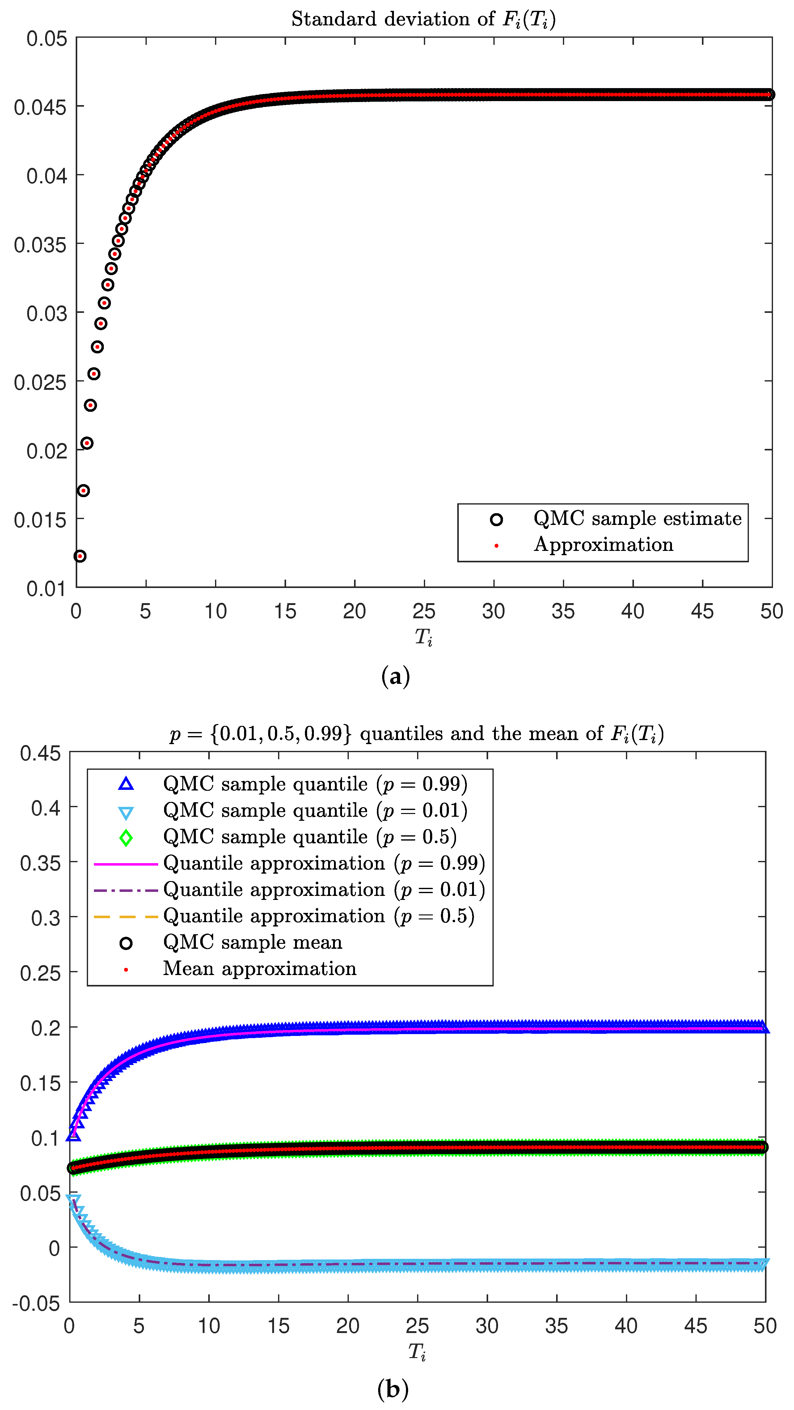
Figure 1. Diagnostic tool for analysing the distribution of long-dated forward LIBORs in the discretized Vasiček model. (a) Comparing the realised forward LIBOR standard deviation approximation to a benchmark QMC sample estimate. (b) Comparing the realised forward LIBOR p = { 0.01 , 0.5 , 0.99 } quantile and mean approximations to their benchmark QMC sample estimates.
Risks 11 00029 g001
Figure 2. Illustrating the evolution of F i ( t ) with a time-homogeneous exponentially decaying instantaneous volatility function under the discretized Vasiček model. (a) Visual representation of (29). (b) Sample path realisations of F i ( t ) , for i = M = 199 .
Risks 11 00029 g002
Figure 3. Diagnostic tool for analysing the distribution of long-dated forward LIBORs in the five-factor DLFM scenario. (a) Comparing the realised forward LIBOR standard deviation approximation to a benchmark QMC sample estimate. (b) Comparing the realised forward LIBOR p = { 0.01 , 0.5 , 0.99 } quantiles and mean approximations to their benchmark QMC sample estimates.
Risks 11 00029 g003
Figure 4. Assessing the lognormal assumption on the distribution of forward LIBORs at two maturities (25 and 50 years) under the five-factor DLFM scenario using Q–Q plots. (a) A lognormal Q–Q plot for the realised QMC sample of the forward LIBOR maturing at 25 years. (b) A lognormal Q–Q plot for the realised QMC sample of the forward LIBOR maturing at 50 years.
Risks 11 00029 g004
Figure 5. Diagnostic tool for analysing the distribution of the long-dated forward LIBORs in the five-factor DLFM scenario using the damped instantaneous volatility function in (36). (a) Comparison of the un-damped (23) and damped (36) instantaneous volatility functions. (b) Comparing the realised forward LIBOR p = { 0.01 , 0.5 , 0.99 } quantiles and mean approximations to their benchmark QMC sample estimates (on the same scale as Figure 3b).
Risks 11 00029 g005
Figure 6. Implications of using the damped instantaneous volatility function (36) on realised forward LIBOR standard deviation and the approximate lognormality at the 50 year maturity under the five-factor DLFM scenario. (a) Comparing the realised forward LIBOR standard deviation approximation to a benchmark QMC sample estimate (on the same scale Figure 3a). (b) A lognormal Q–Q plot for the realised QMC sample of the forward LIBOR maturing at 50 years.
Risks 11 00029 g006
Table 1. Summary of the DLFM volatility and correlation input parameters.
abcd ρ ζ
0.030.081.350.070.400.8
Disclaimer/Publisher’s Note: The statements, opinions and data contained in all publications are solely those of the individual author(s) and contributor(s) and not of MDPI and/or the editor(s). MDPI and/or the editor(s) disclaim responsibility for any injury to people or property resulting from any ideas, methods, instructions or products referred to in the content.