Cox-Based and Elliptical Telegraph Processes and Their Applications

Abstract

This paper studies two new models for a telegraph process: Cox-based and elliptical telegraph processes. The paper deals with the stochastic motion of a particle on a straight line and on an ellipse with random positive velocity and two opposite directions of motion, which is governed by a telegraph–Cox switching process. A relevant result of our analysis on the straight line is obtaining a linear Volterra integral equation of the first kind for the characteristic function of the probability density function (PDF) of the particle position at a given time. We also generalize Kac’s condition for the telegraph process to the case of a telegraph–Cox switching process. We show some examples of random velocity where the distribution of the coordinate of a particle is expressed explicitly. In addition, we present some novel results related to the switched movement evolution of a particle according to a telegraph–Cox process on an ellipse. Numerical examples and applications are presented for a telegraph–Cox-based process (option pricing formulas) and elliptical telegraph process.

1. Introduction

Starting from the motion of a particle according to a telegraph process on an ellipse, random harmonic oscillators can be built on the ellipse. These models have many applications in physics and engineering, and they are also studied using Langevin stochastic differential equations with a harmonic potential, as can be seen in Gitter (2005). In this survey article, the particular case of colored dichotomous noise is also considered as a driving source.

The asymmetric telegraph process is considered in Beghin et al. (2001), and the asymmetric circular telegraph process is considered in De Gregorio and Iafrate (2021). In Watanabe (1968) and Fontbona et al. (2016), the asymptotic analysis of the telegraph motion is deepened. For the application of telegraph processes in finance, see the book Koles and Ratanov (2013).

The Cox process $N_c\left(t\right)$, $t\ge 0$, also known as a doubly stochastic Poisson process, is a generalization of a Poisson process, whose rate $\lambda$ is a positive random variable. The process is named after the statistician David Cox, who first published the model in 1955 (Cox (1955); Pinsky and Karlin (2011)). We consider in this paper the first new telegraph model, so-called Cox-based telegraph process, and its applications in finance, namely, in option pricing. Our second new model is the so-called elliptical telegraph process. The telegraph process on a circle was considered in De Gregorio and Iafrate (2021). Some finite-velocity random motions driven by the geometric counting process were studied in Di Crescenzo et al. (2023). Symmetrical and asymmetrical classical telegraph processes and their applications in option pricing and spread option valuations were considered in Pogorui et al. (2021a, 2021b, 2021c, 2022).

In this work, we consider a simple Cox process, namely, a Poisson process of rate $\lambda =\Theta$, where $\Theta$ is a random variable. We assume that there exists a cumulative distribution function (CDF) $G\left(\theta \right)$ of $\lambda$; hence, the probability distribution of $N_c\left(t\right)$ is as follows:

$$P\left(N_c\left(t\right)=k\right)={\int }_0^{\infty }\frac{{\left(\theta t\right)}^k{e}^{-\theta t}}{k!}dG\left(\theta \right).$$

(1)

We should remark the following properties of $N_c\left(t\right)$

$$\mathbb{E}\left(N_c\left(t\right)\left|\phantom{N_c\left(t\right)\Theta }\right.\Theta \right)=\Theta t$$

and

$$\mathrm{Var}\left(N_c\left(t\right)\left|\phantom{N_c\left(t\right)\Theta }\right.\Theta \right)=\Theta t.$$

Taking into account the well-known conditional variance formula

$$\mathrm{Var}\left(N_c\left(t\right)\right)=\mathbb{E}\left(\mathrm{Var}\left(N_c\left(t\right)\left|\phantom{N_c\left(t\right)\Theta }\right.\Theta \right)\right)+\mathrm{Var}\left(\mathbb{E}\left(N_c\left(t\right)\left|\phantom{N_c\left(t\right)\Theta }\right.\Theta \right)\right),$$

we have

$$\mathrm{Var}\left(N_c\left(t\right)\right)=t\mathbb{E}\left(\Theta \right)+t^2\mathrm{Var}\left(\Theta \right).$$

It is also straightforward to obtain a formula for the conditional probability distribution of $\Theta$ assuming $N_c\left(t\right)=m$, $m=0,1,2,\dots$

$$P\left(\Theta \le x\left|\phantom{\Theta \le x{N}_c\left(t\right)=m}\right.N_c\left(t\right)=m\right)=\frac{P\left(\left\{\Theta \le x\right\}\cap \left\{N_c\left(t\right)=m\right\}\right)}{P\left(N_c\left(t\right)=m\right)}$$

$$=\frac{{\int }_0^{\infty }P\left(\left\{\Theta \le x\right\}\cap \left\{N_c\left(t\right)=m\right\}\left|\phantom{\left\{\Theta \le x\right\}\cap \left\{N_c\left(t\right)=m\right\}\Theta =\theta }\right.\Theta =\theta \right)dG\left(\theta \right)}{{\int }_0^{\infty }\frac{{\left(\theta t\right)}^m{e}^{-\theta t}}{m!}dG\left(\theta \right)}$$

$$=\frac{{\int }_0^x\frac{{\left(\theta t\right)}^m{e}^{-\theta t}}{m!}dG\left(\theta \right)}{{\int }_0^{\infty }\frac{{\left(\theta t\right)}^m{e}^{-\theta t}}{m!}dG\left(\theta \right)}=\frac{{\int }_0^x{\left(\theta t\right)}^m{e}^{-\theta t}dG\left(\theta \right)}{{\int }_0^{\infty }{\left(\theta t\right)}^m{e}^{-\theta t}dG\left(\theta \right)}.$$

Furthermore, if there exists a PDF

$$g\left(x\right)=\frac{dG\left(x\right)}{dx},$$

then the conditional probability density function of $\Theta$ given $N_c\left(t\right)=m$ can be written as

$$f_{\theta |N_c\left(t\right)}\left(x\right|m)=\frac{{\left(xt\right)}^m{e}^{-xt}g\left(x\right)}{{\int }_0^{\infty }{\left(\theta t\right)}^m{e}^{-\theta t}dG\left(\theta \right)}.$$

Suppose that a particle moves in a line as follows: It starts from a point $x_0$ at initial time, and moves with absolute speed $v_0>0$ along directions 1 or −1 with probability $\frac{1}{2}$ until the first Cox switching instant ${\tau }_1$, where $v_k$, $k=0,1,2,\dots$ are independent and identically distributed (iid) random variables that have the same CDF $\Psi \left(v\right)$ and its corresponding PDF $\psi \left(v\right)=\frac{d}{dx}\Psi \left(v\right)$, $v>0$. At instant ${\tau }_1$, the particle can change the direction of movement to the opposite with probability $\frac{1}{2}$ or continues its motion in the same direction with probability $\frac{1}{2}$, and moves with the absolute random velocity $v_1$ until the next Cox switching instant ${\tau }_2$. At ${\tau }_2$, the particle can change the direction of movement to the opposite with probability $\frac{1}{2}$ or continues its motion in the same direction with probability $\frac{1}{2}$ with the absolute random velocity $v_1$ until the next Cox switching, and so on.

We assume that all ${\tau }_k$ and $v_l$, $k,l\ge 0$ are mutually independent.

Let us denote by $x\left(t\right)$ the position of the particle at time t. Then, it is easily seen that

$$x\left(t\right)=\sum _{j=1}^{N_c\left(t\right)}{v}_{k-1}\left({\tau }_k-{\tau }_{k-1}\right)+v_{N_c\left(t\right)}\left(t-N_c\left(t\right)\right),$$

(2)

with ${\tau }_0=0$, and for all $k\in \mathbb{N}\cup 0$, the random variables $v_k$, ${\tau }_k$ are independent.

We will also investigate the telegraph process $Z\left(t\right)$ on an ellipse centered at the origin (we call it elliptical telegraph process)

$$\frac{x^2}{a^2}+\frac{y^2}{b^2}=1,$$

i.e., a random motion of an object or particle with constant absolute velocity and a switching Cox process governing the direction of movements on the ellipse.

This elliptical telegraph process $Z\left(t\right)$ can be represented as

$$Z\left(t\right)=\frac{a+b}{2}{e}^{ix\left(t\right)}+\frac{a-b}{2}{e}^{-ix\left(t\right)},$$

where $x\left(t\right)$ is defined in Equation (2). See Section 4.

2. Characteristic Function

We assume that the PDF $g\left(\theta \right)=dG\left(\theta \right)/d\theta$ does exist. Now, let us denote as

$$\widehat{g}\left(t\right)={\int }_0^{\infty }{e}^{-\theta t}g\left(\theta \right)d\theta ,$$

the Laplace transform of $g\left(\theta \right)$

From Equation (1), we conclude that $\widehat{g}\left(t\right)=P\left(N_c\left(t\right)=0\right).$

Let us define the characteristic function of the process $x\left(t\right)$ by $H\left(t,\alpha \right)=\mathbb{E}\left[e^{i\alpha x\left(t\right)}\right]$. Thus, we have

Theorem 1. 

The characteristic function $H\left(t,\alpha \right)$ satisfies a renewal-type equation as follows:

$$H\left(t,\alpha \right)=\widehat{g}\left(t\right){\int }_0^{\infty }cos\left(\alpha vt\right)\psi \left(v\right)dv$$

$$-{\int }_0^t{\widehat{g}}^{\prime }\left(u\right){\int }_0^{\infty }cos\left(\alpha vu\right)\psi \left(v\right)dvH\left(t-u,\alpha \right)du.$$

(3)

Proof. 

By using the ideas of renewal theory and Equation (2), we obtain

$$H\left(t,\alpha \right)=\mathbb{E}\left[e^{i\alpha \left({\sum }_{j=1}^{N_c\left(t\right)}{v}_{k-1}\left({\tau }_k-{\tau }_{k-1}\right)+v_{N_c\left(t\right)}\left(t-N_c\left(t\right)\right)\right)}\right]$$

$$=\mathbb{E}\left[I_{\left({\tau }_1>t\right)}{e}^{i\alpha v_{0}t}\right]+{\int }_0^t\mathbb{E}\left[I_{\left({\tau }_1\in du\right)}{e}^{i\alpha v_{0}u}\right]H\left(t-u,\alpha \right)$$

$$=P\left({\tau }_1>t\right)\mathbb{E}\left[e^{i\alpha v_{0}t}\right]+{\int }_0^{t}P\left({\tau }_1\in du\right)\mathbb{E}\left[e^{i\alpha v_{0}u}\right]H\left(t-u,\alpha \right)$$

$$=P\left({\tau }_1>t\right){\int }_0^{\infty }cos\left(\alpha vt\right)\psi \left(v\right)dv$$

$$+{\int }_0^{t}P\left({\tau }_1\in du\right){\int }_0^{\infty }cos\left(\alpha vu\right)\psi \left(v\right)dvH\left(t-u,\alpha \right)du$$

$$=\widehat{g}\left(t\right){\int }_0^{\infty }cos\left(\alpha vt\right)\psi \left(v\right)dv-{\int }_0^t{\widehat{g}}^{\prime }\left(u\right){\int }_0^{\infty }cos\left(\alpha vu\right)\psi \left(v\right)dvH\left(t-u,\alpha \right)du.$$

□

Example 1. 

Suppose that $\psi \left(v\right)=\frac{2}{\pi \left(1+v^2\right)}$, $v\ge 0$. Then, we can obtain (see 3.767 in Gradshteyn and Ryzhik (2007))

$${\int }_0^{\infty }cos\left(\alpha vt\right)\psi \left(v\right)dv=\frac{2}{\pi }{\int }_0^{\infty }\frac{cos\left(\alpha vt\right)}{1+v^2}dv=e^{-\left|\alpha \right|t}.$$

In this case, Equation (3) is as follows:

$$H\left(t\right)=\widehat{g}\left(t\right)e^{-\left|\alpha \right|t}-{\int }_0^t{\widehat{g}}^{\prime }\left(u\right)e^{-\left|\alpha \right|u}H\left(t-u\right)du.$$

(4)

Taking into account that $\widehat{g}\left(0\right)=1$, then Equation (4) has solution of the form

$$H\left(t\right)=e^{-t\left|\alpha \right|}.$$

Hence, after calculating the inverse Fourier transform of $H\left(t,\alpha \right)$ (Gradshteyn and Ryzhik (2007)), we obtain the density function $f\left(x,t\right)$ corresponding to

$$f\left(x,t\right)=\frac{t}{\pi \left(t^2+x^2\right)},t>0.$$

Therefore, the PDF $f\left(x,t\right)$ is not dependent on the PDF $g\left(\theta \right)$, and we have the so-called stationary distribution.

We remark that even in the case where the Cox process $N_c\left(t\right)$ is Poisson with rate $\lambda$ and $v=c_0=$ constant, the process $x\left(t\right)$ is not the well-known Goldstein–Kac telegraph process, since the particle may or may not change its direction of velocity at renewal instants. Nevertheless, the Goldstein–Kac-type differential equation for $f\left(x,t\right)$ is as follows (Pogorui et al. (2021b)):

$$\frac{{\partial }^2}{\partial t^2}f\left(x,t\right)+\lambda \frac{\partial }{\partial t}f\left(x,t\right)-c^2\frac{{\partial }^2}{\partial x^2}f\left(x,t\right)=0.$$

(5)

Since the particle starts its motion from $x_0$, we have the following initial conditions: $f\left(x,0\right)=\delta \left(x-x_0\right)$. From Equation (3), it follows that $\frac{\partial }{\partial t}H\left(t,\alpha \right){|}_{t=0}=0$. Hence, $\frac{\partial }{\partial t}f\left(x,t_0\right){|}_{t=0}=0$.

If we have a Cox switching process with distribution (1), it follows from Equation (5) that the Goldstein–Kac-type differential equation for ${\int }_0^{\infty }f\left(\theta ,x,t\right)g\left(\theta \right)d\theta$ (where $f\left(\theta ,x,t\right)$ is the distribution density of the coordinate of the particle assuming $\lambda =\theta$) is the following:

$$\frac{{\partial }^2}{\partial t^2}{\int }_0^{\infty }f\left(\theta ,x,t\right)g\left(\theta \right)d\theta$$

$$+\frac{\partial }{\partial t}{\int }_0^{\infty }\theta f\left(\theta ,x,t\right)g\left(\theta \right)d\theta -c^2\frac{{\partial }^2}{\partial x^2}{\int }_0^{\infty }f\left(\theta ,x,t\right)g\left(\theta \right)d\theta =0.$$

Theorem 2. 

Suppose the rate $\lambda ={\Theta }_n$ has the PDF $g_n\left(\theta \right)$ and a sequence $c_n\to \infty$ as $n\to \infty$ are such that

$$\underset{n\to \infty }{lim}\frac{c_n^2}{{\int }_0^{\infty }\theta g_n\left(\theta \right)d\theta }={\sigma }^2>0.$$

Suppose

$$\underset{n\to \infty }{lim}\frac{\sqrt{\mathrm{Var}\left({\Theta }_n\right)}}{\mathbb{E}\left({\Theta }_n\right)}=0.$$

If ${sup}_n{\int }_0^{\infty }{\left(f\left(\theta ,x,t\right)\right)}^2{g}_n\left(\theta \right)d\theta <\infty$, then $L\left(x,t\right)={lim}_{n\to \infty }{\int }_0^{\infty }f\left(\theta ,x,t\right)g_n\left(\theta \right)d\theta$ satisfies the following diffusion equation:

$$\frac{\partial }{\partial t}L(x,t)-{\sigma }^2\frac{{\partial }^2}{\partial x^2}L\left(x,t\right)=0.$$

(6)

Proof. 

By using the Cauchy–Schwarz inequality, we have

$$\left|\frac{{\int }_0^{\infty }\theta f\left(\theta ,x,t\right)g_n\left(\theta \right)d\theta }{{\int }_0^{\infty }\theta g_n\left(\theta \right)d\theta }-{\int }_0^{\infty }f\left(\theta ,x,t\right)g_n\left(\theta \right)d\theta \right|$$

$$=\left|\frac{\mathbb{E}\left({\Theta }_{n}f\left({\Theta }_n,x,t\right)\right)}{\mathbb{E}\left({\Theta }_n\right)}-\mathbb{E}\left(f\left({\Theta }_n,x,t\right)\right)\right|$$

$$=\left|\frac{\mathbb{E}\left[\left({\Theta }_n-\mathbb{E}\left({\Theta }_n\right)\right)f\left({\Theta }_n,x,t\right)\right]}{\mathbb{E}\left({\Theta }_n\right)}\right|$$

$$\le \frac{\sqrt{\mathbb{E}\left[\left({\Theta }_n-\mathbb{E}({\Theta }_n\right){)}^2\right]}\sqrt{\mathbb{E}\left[{\left(f\left({\Theta }_n,x,t\right)\right)}^2\right]}}{\left|\mathbb{E}\left({\Theta }_n\right)\right|}\to 0$$

as $n\to \infty$.

Therefore,

$$\underset{n\to \infty }{lim}\frac{{\int }_0^{\infty }\theta f\left(\theta ,x,t\right)g_n\left(\theta \right)d\theta }{{\int }_0^{\infty }\theta g_n\left(\theta \right)d\theta }=\underset{n\to \infty }{lim}{\int }_0^{\infty }f\left(\theta ,x,t\right)g_n\left(\theta \right)d\theta ,$$

and by passing to $n\to \infty$ in the equation

$$\underset{n\to \infty }{lim}\frac{1}{{\int }_0^{\infty }\theta g_n\left(\theta \right)d\theta }\left(\frac{{\partial }^2}{\partial t^2}{\int }_0^{\infty }f\left(\theta ,x,t\right)g_n\left(\theta \right)d\theta \right.$$

$$\left.+\frac{\partial }{\partial t}{\int }_0^{\infty }\theta f\left(\theta ,x,t\right)g_n\left(\theta \right)d\theta -c_n^2\frac{{\partial }^2}{\partial x^2}{\int }_0^{\infty }f\left(\theta ,x,t\right)g_n\left(\theta \right)d\theta \right)=0,$$

we obtain Equation (6). □

We should notice that Theorem 2 is a generalization of Kac’s condition (Di Crescenzo et al. (2023); Orsingher (1990); Pogorui et al. (2021b)):

$$\underset{n\to \infty }{lim}\frac{c^2}{\lambda }={\sigma }^2>0,\lambda \to \infty$$

for Equation (5).

Corollary 1. 

According to Theorem 2, if $\frac{c_n}{\mathbb{E}\left({\Theta }_n\right)}{\to }_{n\to +\infty }{\sigma }^2,$ then the telegraph–Cox-based process $x_n\left(t\right)$ weakly converges to $\sigma B\left(t\right),$ where $B\left(t\right)$ is a standard Wiener process. It means that under the conditions of Theorem 2, we have the convergence of the corresponding generators and, hence, the convergence of finite-dimensional distributions of the Cox-based process $x_n\left(t\right)$ to $\sigma B\left(t\right)$.

Example 2. 

Suppose $g_n\left(\theta \right)=I_{[n,n+1]}\left(\theta \right).$ Then, $\mathbb{E}\left({\Theta }_n\right)={\int }_0^{\infty }\theta g_n\left(\theta \right)d\theta =n+\frac{1}{2}$, $\mathrm{Var}\left({\Theta }_n\right)=\frac{1}{12}$. Therefore, ${lim}_{n\to \infty }\frac{\sqrt{\mathrm{Var}\left({\Theta }_n\right)}}{\mathbb{E}\left({\Theta }_n\right)}=0.$

If $c_n\to \infty$ as $n\to \infty$ such that $c_n^2/n\to \frac{{\sigma }^2}{2}>0$ as $n\to \infty$, we have

$$x\left(t\right)\stackrel{w}{\to }W\left(t\right)\sim N\left(0,{\sigma }^{2}t\right).$$

Example 3. 

Let $g_n\left(\theta \right)$ be the PDF of the gamma distribution as follows:

$$g_n\left(\theta \right)=\frac{{\beta }^{{\alpha }_n}}{\Gamma \left({\alpha }_n\right)}{\theta }^{{\alpha }_n-1}{e}^{-\beta \theta },\theta >0,{\alpha }_n>0,\beta >0.$$

Then, $\mathbb{E}\left({\Theta }_n\right)=\frac{{\alpha }_n}{\beta }$ and $\mathrm{Var}\left({\Theta }_n\right)=\frac{{\alpha }_n}{{\beta }^2}$. If ${\alpha }_n\to \infty$ as $n\to \infty$, hence,

$$\underset{n\to \infty }{lim}\frac{\sqrt{\mathrm{Var}\left({\Theta }_n\right)}}{\mathbb{E}\left({\Theta }_n\right)}=0,$$

and Theorem 2 can be applied. That is, if $c_n\to \infty$ and ${\alpha }_n\to \infty$ as $n\to \infty$ such that $c_n^2{\beta }^2/{\alpha }_n\to \frac{{\sigma }^2}{2}>0$ as $n\to \infty$, then we have $x\left(t\right)\stackrel{w}{\to }W\left(t\right)\sim N\left(0,{\sigma }^{2}t\right)$.

3. Numerical Examples: Option Pricing for Cox-Based Telegraph Process

3.1. Numerical Example 1 (Black–Scholes Formula Based on Example 2)

According to Theorem 2 and Corollary 1, if $\frac{c_n}{\mathbb{E}\left({\Theta }_n\right)}{\to }_{n\to +\infty }{\sigma }^2,$ then the telegraph–Cox-based process $x_n\left(t\right)$ weakly converges to $\sigma B\left(t\right),$ where $B\left(t\right)$ is a standard Wiener process. Let us take Example 2 with $\mathbb{E}\left({\Theta }_n\right)=n+1/2.$ If we take $c_n:=\sigma \sqrt{(2n+1)/2},$ where $\sigma >0,$ then $c_n^2/\left(\mathbb{E}\left({\Theta }_n\right)\right){\to }_{n\to +\infty }{\sigma }^2.$ Therefore, with these data, the telegraph–Cox-based process $x_n\left(t\right)$ weakly converges to $\sigma B\left(t\right),$ where $B\left(t\right)$ is a standard Wiener/Brownian motion.

Let us consider the following model for a stock price:

$$S_t^n=S_0{e}^{x_n\left(t\right)},$$

where $x_n\left(t\right)$ is a telegraph–Cox-based process from Example 2. Under the above-mentioned conditions in this Example 2, $c_n^2/\mathbb{E}\left({\Theta }_n\right){\to }_{n\to +\infty }\sigma ,$ we can state that

$$S_t^n=S_0{e}^{x_n\left(t\right)}{\to }_d{\widehat{S}}_t:=S_0{e}^{\sigma B\left(t\right)}.$$

Then, under the risk-neutral measure Q, our stock price ${\widehat{S}}_t$ satisfies the following SDE:

$$d{\widehat{S}}_t=r{\widehat{S}}_{t}dt+\sigma {\widehat{S}}_{t}d{\widehat{W}}_t,\sigma =\frac{v}{\sqrt{\lambda }},$$

where ${\sigma }^2:={lim}_{n\to +\infty }\frac{c_n^2}{\mathbb{E}\left({\Theta }_n\right)}.$

Therefore, we can write the Black–Scholes formula for European call option prices $C_n\left(t\right)$ for our model as

$$C_n\left(t\right)=S_{0}N\left(d_1^n\right)-K{e}^{-r(T-t)}N\left(d_2^n\right),$$

(7)

where

$$d_1^n:=\frac{ln(S_0/K)+(r+c_n^2/\mathbb{E}\left({\Theta }_n\right))(T-t)}{(c_n/\sqrt{\mathbb{E}\left({\Theta }_n\right)})\sqrt{T-t}},$$

$$d_2^n:=d_1^n-(c_n/\sqrt{\mathbb{E}\left({\Theta }_n\right)})\sqrt{T-t},$$

and

$$N\left(x\right)=\Phi \left(x\right)=\frac{1}{\sqrt{2\pi }}{\int }_{-\infty }^x{e}^{-\frac{u^2}{2}}du$$

is the cumulative distribution function of a zero mean normal random variable with unit variance, K is a strike price, and T is the maturity.

We note that $C_n\left(t\right){\to }_{n\to +\infty }C\left(t\right),$ where

$$C\left(t\right)=S_{0}N\left(d_1\right)-K{e}^{-r(T-t)}N\left(d_2\right),$$

(8)

where

$$d_1:=\frac{ln(S_0/K)+(r+{\sigma }^2/2)(T-t)}{\sigma \sqrt{T-t}},$$

$$d_2:=d_1-\sigma \sqrt{T-t},$$

and

$$\sigma :=\underset{n\to +\infty }{lim}\frac{c_n^2}{\mathbb{E}\left({\Theta }_n\right)}.$$

Suppose now that $S_0=\$50,K=\$50,r=0.01,c_n=0.2\sqrt{(2n+1)/2},\mathbb{E}\left({\Theta }_n\right)=n+1/2,\sigma =0.2,T=1.$ Then, according to Equation (8), we have the following European call option price at time $t=0:$

$$C\left(0\right)=50\times 0.5596177-50\times e^{-0.01\times 1}\times 0.4800612=4.21666,$$

or $C\left(0\right)=\$4.2.$ Here, $N\left(d_1\right)=0.5596177,N\left(d_2\right)=0.4800612.$

Below Figure 1 and Figure 2 we present some graphs of dynamics $C_n\left(t\right)$ dependent on $c_n$ and on $\mathbb{E}\left({\Theta }_n\right)$ for different $n=1,2,\dots$

Figure 1. Dependence of $C_n\left(t\right)$ on n (fixed $c_1$).

Figure 2. Dependence of $C_n\left(t\right)$ on n (fixed $\mathbb{E}\left({\Theta }_1\right)$).

3.2. Numerical Example 2 (Black–Scholes Formula Based on Example 3)

Let us consider the following model for a stock price:

$$S_t^n=S_0{e}^{x_n\left(t\right)},$$

where $x_n\left(t\right)$ is a telegraph–Cox-based process from Example 3. Under the condition $\sigma :={lim}_{n\to +\infty }{c}_n^2/\mathbb{E}\left({\Theta }_n\right),$ where $\mathbb{E}\left({\Theta }_n\right)={\alpha }_n/\beta$ and $c_n=\sigma \sqrt{{\alpha }_n/\beta },$$\sigma >0,$ we can state that

$$S_t^n=S_0{e}^{x_n\left(t\right)}{\to }_d{\widehat{S}}_t:=S_0{e}^{\sigma B\left(t\right)}.$$

Then, under the risk-neutral measure Q, our stock price ${\widehat{S}}_t$ satisfies the following SDE:

$$d{\widehat{S}}_t=r{\widehat{S}}_{t}dt+\sigma {\widehat{S}}_{t}d{\widehat{W}}_t,$$

where $\sigma :={lim}_{n\to +\infty }{c}_n^2/\mathbb{E}\left({\Theta }_n\right).$

Therefore, we can write the Black–Scholes formula for European call option prices $C_n\left(t\right)$ for our model:

$$C_n\left(t\right)=S_{0}N\left(d_1^n\right)-K{e}^{-r(T-t)}N\left(d_2^n\right),$$

(9)

where

$$d_1^n:=\frac{ln(S_0/K)+(r+c_n^2/\mathbb{E}\left({\Theta }_n\right))(T-t)}{(c_n/\sqrt{\mathbb{E}\left({\Theta }_n\right)})\sqrt{T-t}},$$

$$d_2^n:=d_1^n-(c_n/\sqrt{\mathbb{E}\left({\Theta }_n\right)})\sqrt{T-t},$$

and

$$N\left(x\right)=\Phi \left(x\right)=\frac{1}{\sqrt{2\pi }}{\int }_{-\infty }^x{e}^{-\frac{u^2}{2}}du$$

is the cumulative distribution function of a zero mean normal random variable with unit variance, K is a strike price, and T is the maturity. Recall that $c_n$ and $\mathbb{E}\left({\Theta }_n\right)$ are defined above.

We note that $C_n\left(t\right){\to }_{n\to +\infty }C\left(t\right),$ where

$$C\left(t\right)=S_{0}N\left(d_1\right)-K{e}^{-r(T-t)}N\left(d_2\right),$$

(10)

where

$$d_1:=\frac{ln(S_0/K)+(r+{\sigma }^2/2)(T-t)}{\sigma \sqrt{T-t}},$$

$$d_2:=d_1-\sigma \sqrt{T-t},$$

and

$$\sigma :=\underset{n\to +\infty }{lim}\frac{c_n^2}{\mathbb{E}\left({\Theta }_n\right)}.$$

Suppose now that $S_0=\$50,K=\$50,r=0.01,{\alpha }_n=2,\beta =2,\sigma =0.2,T=1.$ Thus, $c_n=0.2\sqrt{2/2}=0.2,$$\mathbb{E}\left({\Theta }_n\right)=1,$ and $\sigma =0.2.$ Then, according to Equation (9), we have the following European call option price at time $t=0:$

$$C\left(0\right)=50\times 0.5987-50\times e^{-0.01\times 1}\times 0.5199=\$4.197.$$

Here, $N(d_1,n)=0.598706325682924,N(d_2,n)=0.519938805838372.$

Below Figure 3, Figure 4 and Figure 5 we present some graphs of dynamics $C_n\left(t\right)$ dependent on $c_n$ and on $\mathbb{E}\left({\Theta }_n\right)$ for different $n=1,2,\dots$, and thus, different $c_n$ and $\mathbb{E}\left({\Theta }_n\right).$

Figure 3. Dependence of $C_n\left(t\right)$ on ${\alpha }_n$ (fixed $c_1$).

Figure 4. Dependence of $C_n\left(t\right)$ on $\mathbb{E}\left({\Theta }_n\right)$ (fixed $\mathbb{E}\left({\Theta }_1\right)$).

Figure 5. Dependence of $C\left(t\right)$ on $\sigma$.

Remark 1. 

From a practical point of view, say, according to market trading behavior, as the sojourn time in each state of the process $\xi \left(t\right)$ increases, then the liquidity market decreases, and vice versa, as the holding time in each state decreases, then the liquidity market increases. Moreover, in a trading market structure having high-frequency behavior, our telegraph process model for stock price results is more descriptive than the Black–Scholes model. See our paper for further details (Pogorui et al. (2022)).

4. Telegraph Motion on an Ellipse: Elliptical Telegraph Process

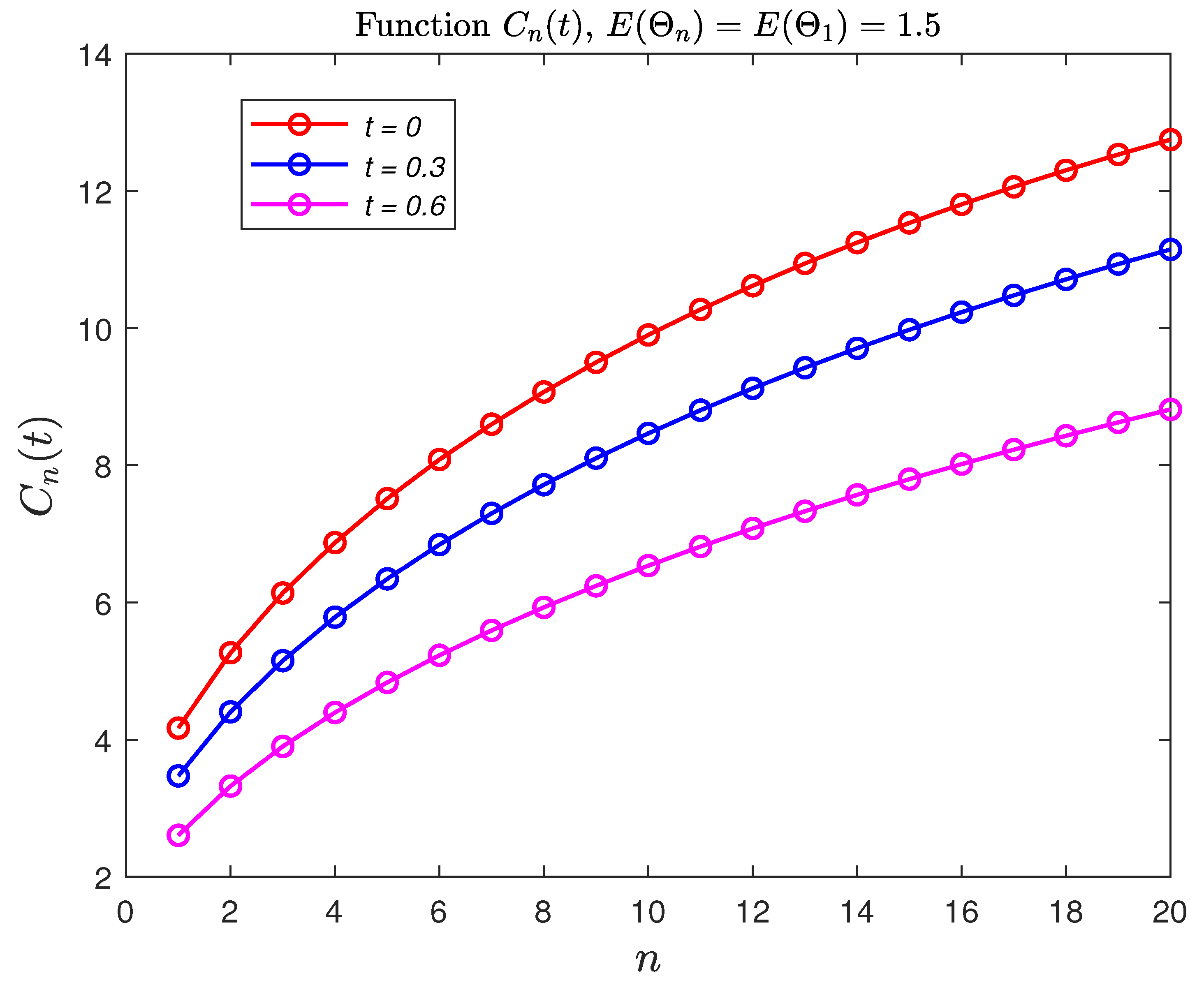
Now, we will investigate the telegraph process $Z\left(t\right)$ on an ellipse centered at the origin

$$\frac{x^2}{a^2}+\frac{y^2}{b^2}=1,$$

i.e., a random motion of an object or particle with constant absolute velocity and a switching Cox process governing the direction of movements on the ellipse.

The stochastic process $Z\left(t\right)$ can be represented as

$$Z\left(t\right)=\frac{a+b}{2}{e}^{ix\left(t\right)}+\frac{a-b}{2}{e}^{-ix\left(t\right)},$$

where $x\left(t\right)$ is defined in Equation (2). By using characteristic functions, we have the expected value

$$\mathbb{E}\left[Z\left(t\right)\right]=\frac{a+b}{2}H(t,1)+\frac{a-b}{2}H(t,-1).$$

Let us consider some examples:

• In the case where $N_c\left(t\right)$ is the Poisson with parameter $\lambda$ and $v=c=$ constant, the characteristic function is of the following form (Pogorui et al. (2021c)):

  $$H\left(t,\alpha \right)=e^{-\frac{\lambda t}{2}}\left(cosh\left(\frac{t}{2}\sqrt{{\lambda }^2-4c^2{\alpha }^2}\right)+\frac{sinh\left(\frac{t}{2}\sqrt{{\lambda }^2-4c^2{\alpha }^2}\right)}{\sqrt{{\lambda }^2-4c^2{\alpha }^2}}\right).$$

  Therefore,

  $$\mathbb{E}\left[Z\left(t\right)\right]=a{e}^{-\frac{\lambda t}{2}}\left(cosh\left(\frac{t}{2}\sqrt{{\lambda }^2-4c^2}\right)+a\frac{sinh\left(\frac{t}{2}\sqrt{{\lambda }^2-4c^2}\right)}{\sqrt{{\lambda }^2-4c^2}}\right).$$

  It is easy to see that using Newton’s binomial theorem, we can calculate moments $\mathbb{E}\left[Z^n\left(t\right)\right]$ for any integer n.
• As it was shown above, in the case where $\psi \left(v\right)=\frac{2}{\pi \left(1+v^2\right)}$, $v\ge 0$, we have $H\left(t,\alpha \right)=e^{-t\left|\alpha \right|}$. Hence,

  $$\mathbb{E}\left[Z\left(t\right)\right]=a{e}^{-t},$$

  $$\mathbb{E}\left[Z^2\left(t\right)\right]=\frac{a^2+b^2}{2}{e}^{-2t}+\frac{a^2-b^2}{2}.$$

A particle’s motion governed by a telegraph process on a circle ($a=b=r$) was studied extensively in De Gregorio and Iafrate (2021), where the authors presented many interesting results. Now, we will develop a partial differential equation that models the motion of a particle on an ellipse governed by a telegraph–Cox stochastic process. Under Kac’s condition, we also obtain a corresponding diffusion equation.

We will call the telegraph–Cox process on an ellipse to $Z\left(t\right)$ with vector representation: $Z\left(t\right)=\left(acos\left(x\left(t\right)\right),bsin\left(x\left(t\right)\right)\right)$.

Consider the following function:

$$\chi \left(t\right)=\left\{\begin{array}{c}0,\mathrm{if}{N}_c\left(t\right)=2k,k\in \mathbb{N}\cup \left\{0\right\}\\ 1,\mathrm{if}{N}_c\left(t\right)=2k-1,k\in \mathbb{N}.\end{array}\right.$$

It is not hard to verify that if $\chi \left(t\right)=0$, then

$$\frac{d}{dt}Z\left(t\right)=\left(-vasin\left(x\left(t\right)\right),vbcos\left(x\left(t\right)\right)\right)=Z\left(t\right)\left(\begin{array}{cc}0& v\frac{b}{a}\\ -v\frac{a}{b}& 0\end{array}\right),$$

and if $\chi \left(t\right)=1$, then

$$\frac{d}{dt}Z\left(t\right)=\left(vasin\left(x\left(t\right)\right),-vbcos\left(x\left(t\right)\right)\right)=Z\left(t\right)\left(\begin{array}{cc}0& -v\frac{b}{a}\\ v\frac{a}{b}& 0\end{array}\right).$$

If $N_c\left(t\right)$ is the Poisson process $N\left(t\right)$ with a rate $\lambda$, then the two-variate process $\left(Z\left(t\right),\chi \left(t\right)\right)$ is a Markov process with the generative operator A as follows (Pogorui et al. (2021b)):

$$A\phi \left(x_1,x_2,0\right)=-v{x}_2\frac{a}{b}\frac{\partial }{\partial x_1}\phi \left(x_1,x_2,0\right)+v{x}_1\frac{b}{a}\frac{\partial }{\partial x_2}\phi \left(x_1,x_2,0\right)+\lambda \phi \left(x_1,x_2,1\right)-\lambda \phi \left(x_1,x_2,0\right),$$

$$A\phi \left(x_1,x_2,1\right)=v{x}_2\frac{a}{b}\frac{\partial }{\partial x_1}\phi \left(x_1,x_2,1\right)-v{x}_1\frac{b}{a}\frac{\partial }{\partial x_2}\phi \left(x_1,x_2,1\right)+\lambda \phi \left(x_1,x_2,0\right)-\lambda \phi \left(x_1,x_2,1\right).$$

Let us consider $f\left(t,\mathit{x},\chi \left(t\right)\right)$, $\mathit{x}=\left(x_1,x_2\right)$ the density function of the particle’s position assuming $\chi \left(t\right)$. Then, we have the following Kolmogorov equation:

$$\frac{\partial }{\partial t}f\left(t,\mathit{x},\chi \left(t\right)\right)=A\phi \left(t,\mathit{x},\chi \left(t\right)\right).$$

In matrix form, this equation can be written as

$$\left(\begin{array}{cc}\frac{\partial }{\partial t}+\frac{av{x}_2}{b}\frac{\partial }{\partial x_1}-\frac{bv{x}_1}{a}\frac{\partial }{\partial x_2}+\lambda & -\lambda \\ -\lambda & \frac{\partial }{\partial t}-\frac{av{x}_2}{b}\frac{\partial }{\partial x_1}+\frac{bv{x}_1}{a}\frac{\partial }{\partial x_2}+\lambda \end{array}\right)\left(\begin{array}{c}f\left(t,\mathit{x},0\right)\\ f\left(t,\mathit{x},1\right)\end{array}\right)=\left(\begin{array}{c}0\\ 0\end{array}\right).$$

It is straightforward to see that $f\left(t,\mathit{x}\right)=f\left(t,\mathit{x},0\right)+f\left(t,\mathit{x},1\right)$ is the probability density function of the particle in $\mathit{x}$.

We know that $f\left(t,\mathit{x}\right)$ satisfies the following equation (Pogorui et al. (2021b)):

$$\det \left(\begin{array}{cc}\frac{\partial }{\partial t}+\frac{av{x}_2}{b}\frac{\partial }{\partial x_1}-\frac{bv{x}_1}{a}\frac{\partial }{\partial x_2}+\lambda & -\lambda \\ -\lambda & \frac{\partial }{\partial t}-\frac{av{x}_2}{b}\frac{\partial }{\partial x_1}+\frac{bv{x}_1}{a}\frac{\partial }{\partial x_2}+\lambda \end{array}\right)f=0,$$

or in an equivalent form as

$$\begin{array}{c}\left(\frac{{\partial }^2}{\partial t^2}+2\lambda \frac{\partial }{\partial t}-v^2\left(\frac{a^2{x}_2^2}{b^2}\frac{{\partial }^2}{\partial x_1^2}-2x_1{x}_2\frac{{\partial }^2}{\partial x_1\partial x_2}+\frac{b^2{x}_1^2}{a^2}\frac{{\partial }^2}{\partial x_2^2}\right)+v^2\left(x_1\frac{\partial }{\partial x_1}+x_2\frac{\partial }{\partial x_2}\right)\right)\\ \times f\left(t,x_1,x_2\right)=0.\end{array}$$

(11)

Under Kac’s condition,

$$\underset{n\to \infty }{lim}\frac{v^2}{\lambda }={\sigma }^2>0,\lambda \to \infty ,v\to \infty ,$$

then from Equation (11), it follows the equation, which can be considered as the diffusion equation on the ellipse,

$$\frac{\partial }{\partial t}f\left(t,x_1,x_2\right)=\frac{{\sigma }^2}{2}\left[\left(\frac{a^2{x}_2^2}{b^2}\frac{{\partial }^2}{\partial x_1^2}-2x_1{x}_2\frac{{\partial }^2}{\partial x_1\partial x_2}+\frac{b^2{x}_1^2}{a^2}\frac{{\partial }^2}{\partial x_2^2}\right)-\left(x_1\frac{\partial }{\partial x_1}+x_2\frac{\partial }{\partial x_2}\right)\right]$$

$$\times f\left(t,x_1,x_2\right).$$

Applications of Elliptical Telegraph Process

Let us consider the following elliptical telegraph processes:

$$Y_n\left(t\right):=\frac{a+b}{2}{e}^{i{\sigma }_{n}x\left(nt\right)}+\frac{a-b}{2}{e}^{-i{\sigma }_{n}x\left(nt\right)},$$

where ${\sigma }_n:=\sqrt{\lambda /n}(1/c)$ and $x\left(t\right)$ is a telegraph process.

Then $Y_n\left(t\right)$ converges weakly, as $n\to +\infty ,$ to Brownian motion on ellipse, $E\left(t\right)$ (or elliptical Brownian motion):

$$E\left(t\right)::=\frac{a+b}{2}{e}^{iB\left(t\right)}+\frac{a-b}{2}{e}^{-iB\left(t\right)},$$

where $B\left(t\right)$ is a standard Brownian motion. The elliptical Brownian motion can be also presented in a vector form:

$$E\left(t\right)=(acos(B\left(t\right),bsin\left(B\left(t\right)\right):=(E_1\left(t\right),E_2\left(t\right)).$$

Here, $E_1\left(0\right)=a$ and $E_2\left(0\right)=0.$ We mention that $E_1\left(t\right)$ and $E_2\left(t\right)$ represent the projections of the elliptical telegraph process $E\left(t\right)$ on the x-axis and y-axis, respectively. Thus, the interpretation can be as a randomized version of an elliptical harmonic oscillator.

Using its formula, we can find the following SDE for $E_i\left(t\right),i=1,2:$

$$\left\{\begin{array}{ccc}\hfill d{E}_1\left(t\right)& =& -\frac{a}{2}cos\left(B\left(t\right)\right)dt-asin\left(B\left(t\right)\right)dB\left(t\right)\hfill \\ \hfill d{E}_2\left(t\right)& =& -\frac{b}{2}sin\left(B\left(t\right)\right)dt-bcos\left(B\left(t\right)\right)dB\left(t\right),\hfill \end{array}\right.$$

or

$$\left\{\begin{array}{ccc}\hfill d{E}_1\left(t\right)& =& -\frac{1}{2}{E}_1\left(t\right))dt-\frac{a}{b}{E}_2\left(t\right)dB\left(t\right)\hfill \\ \hfill d{E}_2\left(t\right)& =& -\frac{1}{2}{E}_2\left(t\right)dt-\frac{b}{a}{E}_1\left(t\right)dB\left(t\right),\hfill \end{array}\right.$$

Therefore, elliptical Brownian motion can be described by those two SDEs.

The wrapped path of $Z\left(t\right)$ on Figure 6 is displayed as the size of the ellipse increases in order to visually distinguish between overlapping arc pieces.

Figure 6. Wrapped path of $Z\left(t\right)$.

Remark 2. 

We note that the telegraph random evolution on a circle was considered in De Gregorio and Iafrate (2021).

5. Conclusions

This paper studied two new models for a telegraph process: Cox-based and elliptical telegraph processes. The paper dealt with the stochastic motion of a particle on a straight line and on an ellipse with random positive velocity and two opposite directions of motion, which is governed by a telegraph–Cox switching process. A relevant result of our analysis on the straight line is obtaining a linear Volterra integral equation of the first kind for the characteristic function of the probability density function (PDF) of the particle position at a given time. We also generalized Kac’s condition for the telegraph process to the case of a telegraph–Cox switching process. We showed some examples of random velocity where the distribution of the coordinate of a particle is expressed explicitly. In addition, we presented some novel results related to the switched movement evolution of a particle according to a telegraph–Cox process on an ellipse. Numerical examples and applications were presented for a telegraph–Cox-based process (option pricing formulas) and elliptical telegraph process. Future work will be devoted to the applications of Cox-based and elliptical telegraph processes in physics, in the context of Langevin SDEs with a harmonic potential, and in finance.

References

1. Beghin, Luisa, Luciano Nieddu, and Enzo Orsingher. 2001. Probabilistic analysis of the telegrapher’s process with drift by means of relativistic transformations. Journal of Applied Mathematics & Stochastic Analysis 14: 11D25. [Google Scholar]
2. Cox, David R. 1955. Some Statistical Methods Connected with Series of Events. Journal of the Royal Statistical Society: Series B (Methodological) 17: 129–57. [Google Scholar] [CrossRef]
3. De Gregorio, Alessandro, and Francesco Iafrate. 2021. Telegraph random evolutions on a circle. Stochastic Processes and their Applications 141: 79–108. [Google Scholar] [CrossRef]
4. Di Crescenzo, Antonio, Antonella Iuliano, and Verdiana Mustaro. 2023. On Some Finite-Velocity Random Motions Driven by the Geometric Counting Process. Journal of Statistical Physics 190: 44. [Google Scholar] [CrossRef]
5. Fontbona, Joaquin, Hélène Guérin, and Florent Malrieu. 2016. Long time behavior of telegraph processes under convex potentials. Stochastic Processes and Their Applications 126: 3077–101. [Google Scholar] [CrossRef] [Green Version]
6. Gitterman, M. 2005. Classical harmonic oscillator with multiplicative noise. Physica A 352: 309–34. [Google Scholar] [CrossRef]
7. Gradshteyn, Izrail Solomonovich, and Iosif Moiseevich Ryzhik. 2007. Tables of Integrals, Series, and Products. Cambridge, MA and Amsterdam: Academic Press, Elsevier. [Google Scholar]
8. Kolesnik, Alexander D., and Nikita Ratanov. 2013. Telegraph Processes and Option Pricing. Heidelberg: Springer, vol. 204. [Google Scholar]
9. Orsingher, Enzo. 1990. Probability law, flow function, maximum distribution of wave-governed random motions and their connections with Kirchoff’s laws. Stochastic Processes and Their Applications 34: 49–66. [Google Scholar] [CrossRef] [Green Version]
10. Pinsky, Mark A., and Samuel Karlin. 2011. An Introduction to Stochastic Modeling, 4th ed. Amsterdam and Cambridge, MA: Elsevier and Academic Press. [Google Scholar]
11. Pogorui, Anatoliy, Anatoliy Swishchuk, and Ramón Martín Rodríguez-Dagnino. 2021a. Transformations of Telegraph Processes and Their Financial Applications. Risks 9: 147. [Google Scholar] [CrossRef]
12. Pogorui, Anatoliy, Anatoliy Swishchuk, and Ramón Martín Rodríguez-Dagnino. 2021b. Random Motion in Markov and Semi-Markov Random Environment 1: Homogeneous and Inhomogeneous Random Motions. London: ISTE Ltd. & Wiley, vol. 1. [Google Scholar]
13. Pogorui, Anatoliy, Anatoliy Swishchuk, and Ramón Martín Rodríguez-Dagnino. 2021c. Random Motion in Markov and Semi-Markov Random Environment 2: High-Dimensional Random Motions and Financial Applications. London: ISTE Ltd. & Wiley, vol. 2. [Google Scholar]
14. Pogorui, Anatoliy, Anatoliy Swishchuk, and Ramón Martín Rodríguez-Dagnino. 2022. Asymptotic Estimation of Two Telegraph Particle Collisions and Spread Options Valuations. Mathematics 10: 2201. [Google Scholar] [CrossRef]
15. Watanabe, Toitsu. 1968. Approximation of uniform transport process on a finite interval to Brownian motion. Nagoya Mathematical Journal 32: 297–314. [Google Scholar] [CrossRef] [Green Version]
Figure 1. Dependence of C n ( t ) on n (fixed c 1 ).
Risks 11 00126 g001
Figure 2. Dependence of C n ( t ) on n (fixed E ( Θ 1 ) ).
Risks 11 00126 g002
Figure 3. Dependence of C n ( t ) on α n (fixed c 1 ).
Risks 11 00126 g003
Figure 4. Dependence of C n ( t ) on E ( Θ n ) (fixed E ( Θ 1 ) ).
Risks 11 00126 g004
Figure 5. Dependence of C ( t ) on σ .
Risks 11 00126 g005
Figure 6. Wrapped path of Z ( t ) .
Risks 11 00126 g006
Disclaimer/Publisher’s Note: The statements, opinions and data contained in all publications are solely those of the individual author(s) and contributor(s) and not of MDPI and/or the editor(s). MDPI and/or the editor(s) disclaim responsibility for any injury to people or property resulting from any ideas, methods, instructions or products referred to in the content.