
Money as Insurance

Faculty of Management and Business, Tampere University, FI-33014 Tampere, Finland
Risks 2022, 10(12), 238; https://doi.org/10.3390/risks10120238
Submission received: 24 October 2022
/
Revised: 28 November 2022
/
Accepted: 12 December 2022
/
Published: 14 December 2022
Abstract
:Liquid money controlled by a trustworthy central bank can serve as an insurance against external surprises such as stock market crashes, bank fails and other setbacks that endanger the yield of illiquid savings. In turbulent times, the insurance property of money is particularly accentuated. The paper constructs a life cycle framework for the analysis of rational and irrational motives to save money, answers to questions about the effects of saving liquid money on labor supply, illiquid saving and education, and examines the inherent cost of saving cash. The main findings are the following. The rational insurance motive to save money increases total savings by replacing deposit saving more than one-to-one. The share of deposit savings depends positively on the expected interest rate, while the share of cash savings is the higher the less there is inflation. Deposit saving correlates positively and education negatively with the expected market interest rate thus affecting the relative proportion of liquid and illiquid saving, but the implicit cost of cash insurance is independent of education. Money illusion adds an internal bias to consumers’ life-time optimization, thus making them save excessively in cash at the cost of market deposits and increasing the cost of using cash as insurance against external uncertainty.
1. Introduction
The fluency of the market mechanism requires that there must be liquid money in circulation enough to meet all transaction needs. By the classical quantity theory of money formalized by Irving Fisher (1914), the activity of money depends on its velocity, which is constant in the short term and remains a merely technical detail. However, reasons for keeping money out of circulation have been acknowledged for long. Alfred Marshall (1890) highlighted precautionary saving, John Maynard Keynes (1930) emphasized that money is a store of value and thus a vehicle of saving and Joan Robinson (1937) discussed the effect of hoarding money on total savings in the economy.
Robert Clower (1967) introduced the famous cash-in-advance constraint (CIA) for economic agents, telling that cash must be held prior to purchasing goods (Kam and Missios 2003). Clower’s contemporary Miguel Sidrauski (1967) provided an alternative supplement to the theory by postulating that holding cash money yields utility just like the consumption of goods and leisure. This means that money with real purchasing power is one argument in consumers’ utility function with standard properties, including diminishing marginal utility and positive cross effects. The latter property means that a marginal increase in one argument causes the marginal utility from another argument to increase. Therefore, a bit more of money should make the marginal utility from consumption of goods or leisure rise. The claim may sound surprising, but it is quite acceptable in the light of standard economic theory, and Holman (1998) finds empirical support for the view, too.
Ayse Imrohoroglu (1992) noted that cash reserves provide insurance against the accidental volatility of illiquid assets. The expected returns of alternative saving methods, such as fixed deposits or other illiquid saving modes are prone to risk and uncertainty, from which cash provides protection. Carl Walsh (2013) followed Baumol (1952) and Tobin (1956) by adding that real money creates utility by providing so called transaction services, thus making the acquisition and use of other utility producing items more convenient. For example, motoring is a lot more carefree when one knows that the accidentally broken car can right away be replaced without sacrifice of other consumption. That can be guaranteed either by an insurance company or by a fat wallet. In any case, one can enjoy consumption and leisure more relaxed, implying that the enjoyment should also be more luxurious.
From the insurance perspective, holding cash money can be a rational mode of saving, especially in turbulent times. In fact, both the 2008 financial crisis and the 2020 pandemic have made people respond to grown uncertainty by increasing their cash holding, and the Ukrainian crisis has even accelerated the development, at least in Europe. In all times, money has attracted people also by irrational motives. Behavioral economics (Tversky and Kahneman 1992) provides many explanations for hoarding money, but this paper restricts to a classical description of irrational behavior, namely money illusion. According to Fisher (1928), people tend to evaluate economic matters in nominal rather than real values, while nominal monetary values should have no role in rational market behavior.
The aim of the paper is twofold. First, it aims to extend the standard life cycle consumption model originated by Fisher (1930) to serve as an illustrative framework for the analysis of motivated saving of cash money. For simplicity, the focus is on saving so that taking loans is omitted, as well as the opportunity cost of leisure. Thus, the main motivation of the paper is to lay grounds for further studies. Examples of more sophisticated analyses include Zhao and Siu (2020), which investigated consumption-leisure-investment choice with time-varying preferences, and Orland and Rostam-Afschar (2021) which considered flexible work arrangements. Moreover, Baiardi et al. (2019) examined various extensions to the theory of precautionary saving, including multiple variables affecting household utility, and Boar (2021) analyzed precautionary saving motives across generations. Vasilev (2022) provided a DSGE-model analysis of economic fluctuations with real money balances entering in a non-separable way with consumption and leisure.
In this paper, the utility creating property of money is modelled in a standard way without plugging money in the utility function. Instead, money enters the budget constraint just like any savings do. Second, the paper aims to answer to important questions about the consequences of rational and irrational saving of money on labor supply, illiquid saving, and investment in education. In particular, the aim is to show the inherent cost of the use of cash money as a saving mode. In the framework, the cost from holding cash can be measured in terms of compensating variation (Varian 2019).
The main findings of the paper are the following. In the elementary model without education, it is found that the rational insurance motive to save money increases total savings by replacing deposit saving more than one-to-one. The share of deposit savings depends positively on the expected interest rate. On the other hand, the share of cash savings is the higher the less there is rationally anticipated inflation, which means that as smaller inflation makes cash insurance cheaper, consumers purchase better security. Incorporating education into the model shows that deposit saving correlates positively and education negatively with the expected market interest rate, thus affecting their relative proportion. The introduction of education does not affect the implicit price paid for cash insurance. Incorporating money illusion, i.e., misjudgment of the inflation rate, makes consumers save excessively in cash at the cost of market deposits. Quite expectedly, money illusion increases the cost of using cash as insurance.
The paper proceeds as follows. Section 2 constructs the basic life cycle model of cash as rational insurance with perfect foresight on inflation but external uncertainty about the yield of market deposits. Section 3 adds education into the model with external uncertainty about its yield. Section 4 incorporates consumers’ internal bias into the analysis, namely, irrationality caused by money illusion. Section 5 discusses and concludes the findings.
2. Money and Rational Precaution
In an elementary life cycle consumption model, the representative consumer allocates her lifetime incomes to consumption according to her time preference (Fisher 1930; Burda and Wyplosz 2017). For simplicity, the consumer’s life cycle is divided into two parts, period 1 and period 2, and all decisions are made at the beginning of period 1. Moreover, time use in both periods is fixed to acquiring labor income so that leisure time is not an argument in the utility function. Thus, the representative consumer maximizes:
u(q1, q2)
In the utility function, q1 is consumption in the first period, and q2 is consumption in the second period. The standard assumptions u1, u2 > 0; u11, u22 < 0; u12, u21 > 0 hold, where the subscripts denote first and second order derivatives according to the two arguments of the utility function. Moreover, the utility function is assumed homothetic, meaning that plain income effects do not change the consumer’s time preference in the short term. This is a reasonable assumption in the static model.
The holding of liquid cash money is justified by external uncertainty concerning the returns of illiquid deposits. The amount of cash saving is accounted in the budget constraints so that it becomes a choice variable just like all saving. Assuming that the consumer’s productivity remains unchanged over the life cycle and normalizing both time and labor income to unity in both periods, the income endowment is E = (1, 1). The period budget constraints read:
q1 = 1 − m − s
q2 = 1 + αm + (1 + r)s
In Equation (1), 1 is labor income, m is cash saving and s is illiquid deposit saving. In Equation (2), α = 1/(1 + π) where π is the inflation rate between the periods and 0 < α ≤ 1. Therefore, αm is the real return from holding cash. On the other hand, r ≥ 0 is the expected real market rate of return and (1 + r)s is the expected return from illiquid saving. Solving for s from (1) and substituting into (2) produces the consumer’s life-time budget constraint:
q2 = 1 + αm + (1 + r)(1 − m) − (1 + r)q1
Therefore, the optimization problem of the representative consumer reads:
Max u(q1, q2) s.t. q2 = 1 + αm + (1 + r)(1 − m) − (1 + r)q1
The solution to the optimization problem can be analyzed in two steps. First, the consumer chooses the amount of cash saving in order to protect herself from all possible extreme events concerning the refund of illiquid savings. The rule for optimal cash holdings is derived by plugging (1) and (2) into the utility function and solving optimal m. This produces:
Rule (4) tells that, at the optimum, the slope of the indifference curve , which measures the consumer’s time preference, must be equal to the marginal rate of return of cash saving.
Second, the consumer decides on the optimal timing of her consumption by deciding on illiquid saving along the life-time budget constraint, which is now restricted by the initial of m. The rule for optimal illiquid saving is derived by plugging (3) into the utility function and solving for q1. This produces:
Rule (5) tells that, at the optimum, the slope of the indifference curve must be equal to the expected return of illiquid savings (1 + r).
Note that α = (1 + r) only if α = 1 and r = 0. If so, all savings would be in cash. When α (1 + r), the rules (4) and (5) hold in optimal solutions, which occur on different utility levels depicted by the set of homothetic indifference curves portraying the consumer’s time preference.
Figure 1 illustrates the analytical treatment of the representative consumer’s recursive life-time optimization.
Figure 1 illustrates the representative consumer’s recursive life-cycle decision making, which can be analyzed in two steps. First, the consumer chooses the amount of her cash savings. Assuming that inflation is perfectly anticipated, consumption possibilities can be transferred forwards by cash money along the return line, which starts from point E and rises leftwards. The slope of the line is 0 < α < 1 due to inflation so that the return from saving money is negative. The optimum condition (4) holds at point c, where the highest possible indifference curve ü from the set of the homothetic utility function touches the return line. The optimal amount of cash saving is m, which also measures the amount of working time devoted to the accumulation of cash money. Thus, the utility level ü(1 − m, 1 + αm) is the safeguard for life-time consumption utility. Note that the external uncertainty may concern not only the market rate of return r, but also the return of capital so that ü is the bottom safeguard against total vanish of the deposits.
Second, the consumer decides on her illiquid saving according to its expected return 1 + r. Since the cash saving m is now given, the labor income that can be used to market saving in period 1 is restricted. Therefore, the life-time budget constraint with the slope −(1 + r) is shifted inwards so that it goes through point c instead of point E. The optimum condition (5) for illiquid saving holds in point b, where the highest possible indifference curve from the set of the homothetic utility function touches the solid life-time budget constraint. The optimal amount of illiquid deposit saving is s, which also determines the amount of work needed for the accumulation of deposit savings.
The consumer’s recursive life-time optimization at the beginning of period 1 produces total savings σ = m + s in period 1 to be consumed in period 2. The return from cash saving is αm in terms of secure consumption in period 2, and the return from deposit saving is (1 + r)s in terms of expected consumption in period 2. Thus, consumption in period 1 is q1 = 1 − m − s, and the expected consumption in period 2 is q2 = 1 + αm + (1 + r)s.
In Figure 1, the consumer’s expected utility at the final optimum point b is u(q1, q2). For comparison, a dashed life-time budget constraint going through point E is drawn to illustrate the hypothetical case, where there would be no uncertainty about the yield of illiquid deposits and, thus, no need for insurance. In that case, the optimization would include only one analytical step according to rule (5). The optimum would occur at point ε, where the highest possible indifference curve from the set of the homothetic utility function touches the dashed life-time budget constraint. The consumer would then reach to the higher utility level u* by depositing sɛ and receiving the warranted (1 + r)sε in return.
The analysis shows that since m + s = σ > sε, the rational insurance motive to save money increases the amount of total savings compared to the case of perfect foresight. Therefore, secure cash saving replaces insecure deposit saving more than one-to-one. It can also be inferred from Figure 1 that the higher is the expected market interest rate r the larger is the share of deposit savings in total savings σ/s, and vice versa. The results are clear under the assumption of homothetic preferences saying that the consumer’s time preference is not affected by pure income effects.
Another important observation can be deduced by considering the value of the inflation parameter α. From Figure 1, one can infer that the closer the value of α is to unity; that is, the steeper is the yield line for cash, the further leftwards from E point c along the solid life-time budget constraint settles. This is due to the substitution effect caused by the fall in the relative price of cash saving. The final optimum would then be below point b along the dashed line from the origin implying lower expected consumption and utility. The implication is that both cash and deposit saving would increase, but the share of m in σ would grow, because less inflation means higher return to cash savings.
The comparison between the cases of perfect foresight and external uncertainty reveals the implicit price of the consumer’s insurance against misfortunes. It can be measured by compensating variation (CV); that is, by the distance between the solid and dashed budget constraints in Figure 1. The horizontal difference between the constraints can be calculated in terms of period 1 consumption by solving q1 from (3) in both cases. The point of intersection of the solid constraint with m > 0 along the horizontal axis is:
q1 = 1 − m + (1 + αm)/(1 + r)
The respective intersection point of the dashed constraint with m = 0 reads:
q1 = (2 + r)/(1 + r)
Subtracting the former expression from the latter one produces, after some manipulation:
The compensating variation CV in (6) measures the amount of period 1 consumption that would compensate the discrepancy between u and u*. Thus, it gives the cost that the consumer willingly pays for secured consumption. Expression (6) also tells that if α = 1 and r = 0, the implicit unit price of the insurance 1 − α/(1 + r) and, thus, the cost of holding m is zero. When α (1 + r), the unit price depends negatively on α and positively on r. Since α is the inverse measure of inflation, the conclusion is that both lower inflation and lower expected interest rate mean lower unit price, and vice versa.
However, Figure 1 also reveals that a lower inflation rate means a higher implicit cost [1 − α/(1 + r)]m of the insurance. This may sound surprising, but the homothetic utility function is uncompromising: lower inflation means a higher value of α and, thus, a steeper yield line, along which the cash insurance optimum would set north-west from point c, and the outcome would be a broader CV difference along the horizontal axis. Thus, consumption utility u would be further apart from u*, while the safeguard utility level ü would be higher. The economic intuition is that, as smaller inflation makes the unit price of cash insurance cheaper, the consumer purchases broader security against the worst possible scenario.
In fact, holding cash “just in case” does not differ much from normal insurances. The main difference is that while the pricing of commercial insurance products is distorted by adverse selection and moral hazard, cash saving can be planned independently. Another difference is that commercial force majeure—insurances do not usually cover total unpredictability or “black swans” (Barr 2001). In that respect, holding cash can be a better option.
3. Money, Education and Saving
Basic life-cycle models usually also include the possibility to invest in one’s own productivity (Burda and Wyplosz 2017). A simplifying assumption is that one can use part of her time in period 1 in education to cultivate her skills and enjoy the product of the investment in period 2. Another reasonable assumption is that the time used in education fosters productivity and, thus, wages with diminishing marginal returns. Denoting the time used in education in period 1 by e, the expected product from the investment in period 1 to period 2 is w2 = w(e) with w′ > 0, w″ < 0, where the sub-primes denote first and second order derivatives. With these amendments, the representative consumer’s periodic budget constraints read:
q1 = 1 − e − m − s
q2 = w2 + αm + (1 + r)s
Solving s from (7) and plugging into (8) produces the life-time budget constraint:
The consumer solves the problem:
Now, the solution to the representative consumer’s recursive optimization problem can be analyzed in three steps.
The first step is again to decide on cash saving, which necessitates time use in work to earn money in period 1. Plugging (7) and (8) into the utility function and solving m yields:
Being similar to rule (4) above, rule (10) tells that the slope of the highest possible indifference curve from the set of homothetic utility function must be equal to the marginal rate of return of cash saving.
The second step concerns the optimization of education time. This is performed by maximizing the life-time income from the right-hand side of (9) with respect to e. Recalling the expected yield w2 = w(e), the optimum condition is:
Rule (11) says that, in the optimum, the marginal rate of return from the time spent in education must equal the slope of the life-time budget constraint, which measures the expected opportunity cost of education in terms of deposit saving.
Finally, the consumer optimizes the timing of consumption along the life-time budget constraint. Plugging (9) into the utility function and solving for q1 produces:
Like rule (5) above, rule (12) determines the optimal amount of deposit saving. When the secure yield of cash savings differs from the expected market yield, α (1 + r), the conditions (10) and (12) refer to solutions that occur on different utility levels among the set of indifference curves describing the homothetic utility function. On the other hand, (11) and (12) depict separate education and consumption optimums along the expected budget constraint, thus obeying the Fisherian condition:
Figure 2 illustrates the representative consumer’s recursive optimization including cash saving, education, and the timing of consumption via deposit saving. The consumer is assumed to be perfectly aware of inflation, while the product of education and the market yield from savings are uncertain. Thus, there is a rational motive for saving cash money.
In Figure 2, the first step of the consumer’s recursive optimization is to decide on the amount of cash saving. This is performed by devoting part of the time available in period 1 to work so that the accumulated labor income covers the chosen amount of cash. By (10), the optimum is at point c and the optimal amount of cash holdings is m, which also measures the time used in work to accumulate the needed cash. The cash saving m is transferred to period 2 as αm, where 0 < α < 1. This secures the utility level ü as protection for any external uncertainties.
On the second step, the consumer optimizes on education time in period 1. Due to the use of time in work necessitated by cash saving, the time available for other purposes is now 1 − m. Therefore, the time investment in education can start from point c, and the expected product of the investment develops leftwards along the deceleratingly rising solid curve w(e). Condition (11) holds in point a, where the expected marginal product of education equals its expected opportunity cost. Labor income in period 1 is w1 and the expected labor income in period 2 is w2 = ew′.
The final analytical step concerns optimal timing of consumption by deposits. Since the optimization of education has shifted the life-time budget constraint outwards to go through point a, condition (12) holds in point b. Deposit saving in period 1 is s with the expected return (1 + r)s in terms of period 2 consumption. Thus, consumption in period 1 is q1 = (1 − e) − (m + s) and the expected consumption in period 2 is q2 = αm + ew′ + (1 + r)s.
The analysis yields the following notions. First, the introduction of education does not affect cash insurance saving. Rule (10) says that the optimization on the amount of cash m depends on the perfectly anticipated inflation parameter α, which has nothing to do with either education or deposit saving. Therefore, ü depicts the bottom safeguard for the worst possible scenario, where the deposits would be wiped out and employment corresponding to the chosen education would not be available in period 2.
Second, to put it the other way round, the rational cash insurance does not affect the consumer’s choice of education, because the model does not include leisure time, thus omitting the opportunity cost of leisure. Figure 2 provides a comparison to the case of perfect foresight, where the dashed product curve of education starts from point E, and education and saving decisions are made along the budget line tangent to the curve. Then, cash saving makes the start of the product curve w(e) shift north-west from point E to point c. Since the curve retains its shape, rule (11) holds at point ϶, and the point pair E and ϶ produces the same amounts of e and ew′ as the point pair c and a with cash insurance. Namely, e϶ = e and e϶w′ = ew′ = w2 in Figure 2.
Third, Figure 2 shows again that uncertainty makes the consumer save more in total compared to the case of perfect foresight; that is, s + m = σ > sε. The effect remains qualitatively the same as in Figure 1 due to the neutrality of cash saving on education. However, Figure 2 also reveals that a fall in the expected market interest rate would make the investment in education e grow at the expense of deposit saving s. From the macroeconomic point of view, the partial replacement of s by e would mean replacement of physical capital accumulation by human capital accumulation. In the case of a rise in the expected interest rate, the effects would be reversed.1
Lastly, the above findings pave way to the conclusion that the introduction of education into the model does not affect the voluntary implicit price paid for the cash insurance. In technical terms, the CV measure of the model should equal the measure derived from Figure 1. This can be verified by recalling (9) and calculating the horizontal intersection point with money and education:
q1 = (1 − e − m) + (w2 + αm)/(1 + r)
This refers to the solid life-time budget constraint in Figure 2. The respective intersection of the dashed budget line that depicts the case with m = 0 is:
q1 = (1 − e) + w2/(1 + r)
Subtracting the former from the latter gives:
Since the result is the same as in (6) before, the cost of the cash insurance in terms of period 1 consumption is independent of the decision on education. The economic intuition is that, since the yield from both education and deposit saving decision is uncertain, the optimal amount of cash savings m that secures ü provides insurance for all negative surprises, including those that concern the yield of education.
4. Money Illusion
In the previous sections, the assumption has been that the consumer faces only external uncertainty concerning the yields of deposit saving and education, while inflation is perfectly anticipated. In those circumstances, cash is a rational insurance mode of saving. Still, there also exist various internal biases that make people hoard money more than what would be reasoned by rational arguments. Money illusion is one such psychological factor, which is broadly accepted in economic theory and confirmed by many empirical verifications (Fisher 1928; Blanchard et al. 2010; Begg et al. 2014). Money illusion makes people concentrate on the nominal value of money instead of its real purchasing power. According to Akerlof and Shiller (2009), the misjudgment of inflation causes market anomalies because it distorts the market by making the recursive price mechanism sticky.
Money illusion distorts especially long-term decisions, in which expected inflation should naturally be accounted. In static sense, the implications of money illusion can be dealt with the life-cycle model presented in the previous section, and Figure 3 illustrates the effects of the matter. For simplicity, the representative consumer is assumed to suffer from absolute money illusion, since allowing for partial money illusion would not change the main findings.
Absolute money illusion means that consumers falsely presume one-to-one yield from saving money forwards. Figure 3 presents this so that the representative consumer presumes α = 1 instead of the fact that 0 < α < 1. In the figure, the demarcation is quite notable for clarity. The consumer’s choices under money illusion are presented by superscript i.
On the first step of her recursive optimization, the internally biased consumer chooses the amount of money along the yield line that rises leftwards from E by the slope −1. As a result, money illusion misleads the consumer to choose mi according to the point ci instead of choosing the rationally motivated m according to point c. This means that the difference mi − m > 0 is due to irrationality.
On the second step, the consumer optimizes on education taken that the choice mi has made the yield curve of education start from point ci instead of point c. By (11), the choice of education is not distorted by money illusion, because it is based on the expected real interest rate that is externally given to the consumer. Thus, the consumer chooses education according to the point ai instead of choosing it according to point a. Nevertheless, ei = e and eiw′ = ew′ because the model omits the opportunity cost of leisure.
The third step of the consumer’s recursive optimization is based on (12), but the homotheticity of the utility function causes money illusion to affect the choice. The consumer chooses si according to bi instead of choosing s according to b, which means that si < s. While excess cash saving mi cuts available working time, thus placing point ci north-west from point c, homothetic preferences keep points bi and b on the dashed line starting from the origin.
The analysis produces the following findings. First, money illusion misleads the representative consumer to save excessively in cash and shortly in market deposits. This is because the consumer underestimates the cost of holding money and errs to take an overly covering insurance mi against uncertainty. Moreover, albeit total savings are smaller under money illusion than under perfect foresight, that is, mi + si = σi < σ = m + s, the share of cash of total savings is larger under money illusion, mi/σi > m/σ. The qualitative effects of changes in the expected market interest rate remain the same as discussed in the previous sections.
Second, the static life-cycle model, where all decisions are made at the beginning of period 1, shows only the optimal plan but not the true outcome in period 2. However, an external observer can evaluate the cost of money illusion by the means of the CV analysis. From (9), the calculation of the horizontal intersection point of the dashed constraint in Figure 3 produces the control case without money illusion:
q1 = 1 − m − e + (w2 + αm)/(1 + r)
Under absolute money illusion, (9) turns to q2 = w2 + mi + (1 + r)(1 − mi − e − q1) where mi denotes the cash saved in period 1 and anticipated to be recollected as such in period 2. Calculation and manipulation produce the horizontal intersection point of the solid constraint:
q1 = (1 − e) + (w2 − rmi)/(1 + r)
Subtracting the latter formula with money illusion from the former without such internal bias, that is, calculating the horizontal difference between the dashed and solid budget constraints of Figure 3, produces:
Note that the CVi in (14) is calculated inversely to catch the fact that money illusion lures the consumer to reach beyond truly attainable consumption possibilities, thus motivating excessive saving of money. On the other hand, the CV in (6) measures what would be the cost of rational precaution to external uncertainty, that is, the horizontally measured inward shift of the dashed constraint caused by holding m. Therefore, the total cost of holding mi amounts to CV + CVi. Since the CV in (6) cancels out the first term of the CVi in (14), the remainder is:
The remainder measures the excess burden caused by money illusion. Thus, in terms of period 1 consumption, the excess cost caused by money illusion equals the discounted expected marginal opportunity cost of the overly saved amount of money mi. The result is economically intuitive, and the result holds qualitatively under partial money illusion.
5. Conclusions
This paper examined the role of cash money as a mode of saving. A simple life cycle consumption model was constructed, where people live for two periods and allocate their life-time incomes into life-time consumption to maximize utility from consumption during the two periods. In the static model, all decisions are made at the start of the life cycle. The optimal allocation of consumption is guided by constant time preferences depicted by a homothetic utility function, and income can be timed to consumption forwards by saving or backwards by lending. For practical reasons, the paper focused on the decision making of a representative saver. In the model, life-time labor income was also endogenous, because consumers could cultivate their skills in the first period to improve their productivity and thus wages in the second period.
Both rational and irrational motives for holding cash money were studied. The rational motive was assumed to arise from uncertainty caused by reasons that are external to the decisionmaker. The external uncertainty was assumed to blur the expected yield from illiquid savings and investment in education. In both cases, the worst scenario was that not only the interest, but also the invested capital would vanish. Thus, saving cash money can provide a rational insurance against misfortunes of any kind. As an irrational motive for saving cash, a factor internal to the decisionmaker was introduced, namely, psychological bias caused by money illusion.
The consumer’s intertemporal optimization was first studied in an elementary case, where life-time income was fixed, and the optimization problem was to decide on optimal saving from period 1 to period 2. In particular, the optimization concerned the composition of total savings consisting of liquid cash money and illiquid market deposits, when the market yield of the deposits was uncertain. Under these circumstances, it is rational to save cash as an insurance for future consumption such that accords to the time preference. It was found that the cash insurance increases total savings compared to the case of perfect foresight. Moreover, it was found that the share of deposit savings in total savings depends positively on the expected market rate of return, and that the share of cash depends negatively on inflation.
The implicit cost of the consumer’s rational cash insurance against uncertainty was measured by compensating variation, which gives the amount of extra consumption that would compensate the discrepancy of the realized utility level from the perfect foresight control level. Calculating in terms of period 1 consumption, the unit price of holding money was found to depend positively on both perfectly anticipated inflation and expected market interest rate. However, the cost of the cash insurance was found to depend negatively on the inflation rate: the calculus of compensating variation under constant time preference showed that the implicit voluntary cost of the cash insurance is the higher the smaller is the perfectly anticipated inflation rate.
Introducing investment in education into the model showed that the decision on education is independent of cash saving, taken that the opportunity cost of leisure is omitted. This implied that the findings concerning liquid and illiquid saving remained qualitatively the same as without education. Quite expectedly, it was found that a lower expected market interest rate would make the investment in education grow at the expense of deposit saving, and vice versa. It was also concluded that the introduction of education into the model does not affect the voluntary implicit unit price and cost of the cash insurance. That is, the respective compensating variation remained unaltered. The economic intuition is that, since the yields from both education and deposit saving decisions are uncertain, the optimal amount of cash savings provides insurance for all extreme events in period 2, including total vanish of the deposits and inability to obtain a job corresponding to education.
Lastly, the implications of internal irrationality, namely, money illusion, were studied. It was found that money illusion misleads the representative consumer to save excessively in cash and shortly in market deposits, because she underestimates the cost of holding money and errs to take an overly covering insurance against external uncertainty. Moreover, albeit total savings were smaller under money illusion compared to perfect foresight, the share of cash in total savings was larger. The qualitative effects of changes in the expected market interest rate were not changed. Most importantly, money illusion was found to increase the cost of the cash insurance. The excess cost caused by the internal psychological was found to equal the discounted expected opportunity cost of the overly saved amount of money. To generalize, money illusion becomes more costly the deeper it is. The findings are relevant because empirical evidence suggests that, at least with creeping inflation, money illusion is a persistent feature in people’s behavior.
To conclude, people can use money as a rational insurance against external uncertainties, but human psychology may internally delude them to excessive cash saving. The paper managed to present a simple and illustrative life cycle model for basic analyses of holding cash money for rational and irrational reasons. Overall, the analyses stuck to the case of a final saver; that is, borrowing was omitted at the final stage of the recursive decision making but allowing for borrowing (or borrowing constraints) would not change the results fundamentally.
The main pitfall of the model is that it omits leisure, which, undeniably, is an important complement to consumption. The cost of this simplifying assumption must be accounted when assessing the general validity of the results. Moreover, the static model is too rigid to present the final outcomes neither at the end of the life span nor happenings along the span. In real life, people presumably learn about their disappointments in the longer run, and they surely err and correct their decisions repeatedly during the run as well. For example, dynamic life-cycle models, DSGE-modeling, rigorous econometrics, experiments and other such devices must be used to obtain a clearer picture of the true state of the matter, but those inquiries are left for further studies. However, the static view taken in this paper may not be too far from reality, where people usually buy expensive insurances from insurance companies against sad incidences, which they wish never to happen.
Funding
This research received no external funding.
Data Availability Statement
The study did not report any data.
Conflicts of Interest
The author declares no conflict of interest.
| 1 | The comparative static properties of the model can be checked by totally differentiating (11) and (12) with recall of (13) and taking m fixed in (7) and (8). Denoting −u11 + 2(1 + r)u12 − (1 + r)2u22 = A > 0 and u12 − (1 + r)u22 = B > 0 and using Cramer’s rule produces:
|
References
- Akerlof, George, and Robert Shiller. 2009. Animal Spirits. Princeton: Princeton University Press. [Google Scholar]
- Baiardi, Donatella, Marco Magnani, and Mario Menegatti. 2019. The theory of precautionary saving: An overview of recent developments. Review of Economics of the Household 18: 513–52. [Google Scholar] [CrossRef]
- Barr, Nicholas. 2001. Welfare State as Piggy Bank. Oxford: Oxford University Press. [Google Scholar]
- Baumol, William. 1952. The Transactions Demand for Cash: An Inventory Theoretical Approach. Quarterly Journal of Economics 66: 545–56. [Google Scholar] [CrossRef]
- Begg, David, Gianluigi Vernasca, Stanley Fischer, and Rudiger Dornbusch. 2014. Economics. New York: McGraw-Hill Education. [Google Scholar]
- Blanchard, Oliver, Alessia Amighini, and Francesco Giavazzi. 2010. Macroeconomics, a European Perspective. London: Pearson Education Ltd. [Google Scholar]
- Boar, Corina. 2021. Dynastic Precautionary Savings. The Review of Economic Studies 88: 2735–65. [Google Scholar] [CrossRef]
- Burda, Michael, and Charles Wyplosz. 2017. Macroeconomics—A European Text. Oxford: Oxford University Press. [Google Scholar]
- Clower, Robert. 1967. A Reconsideration of the Microfoundations of Monetary Theory. Western Economic Journal 6: 1–8. [Google Scholar] [CrossRef]
- Fisher, Irving. 1914. The Purchasing Power of Money. Bulletin of American Mathematical Society 7: 377–81. [Google Scholar]
- Fisher, Irving. 1928. The Money Illusion. New York: Adelphi. [Google Scholar]
- Fisher, Irving. 1930. The Theory of Interest. New York: Macmillan. [Google Scholar]
- Holman, Jill. 1998. GMM Estimation of a Money-in-the-Utility-Function Model: The Implications of Functional Forms. Journal of Money, Credit and Banking 30: 679–98. [Google Scholar] [CrossRef]
- Imrohoroglu, Ayse. 1992. The Welfare Costs of Inflation under Imperfect Insurance. Journal of Economic Dynamics and Control 16: 79–91. [Google Scholar] [CrossRef]
- Kam, Eric, and Paul Missios. 2003. Wealth effects in a cash-in-advance economy. Economics Bulletin 5: 1–7. [Google Scholar]
- Keynes, John Maynard. 1930. Treatise of Money. London: Macmillan. [Google Scholar]
- Marshall, Alfred. 1890. Principles of Economics. London: Macmillan. [Google Scholar]
- Orland, Andreas, and Davud Rostam-Afschar. 2021. Flexible Work Arrangements and Precautionary Behavior. Theory and experimental evidence. Journal of Economic Behavior & Organization 191: 442–81. [Google Scholar]
- Robinson, Joan. 1937. Introduction to the Theory of Employment. London: Macmillan. [Google Scholar]
- Sidrauski, Miguel. 1967. Rational Choice and Patterns of Growth in a Monetary Economy. American Economic Review 57: 534–44. [Google Scholar]
- Tobin, James. 1956. The Interest-Elasticity of Transactions Demand for Cash. The Review of Economics and Statistics 38: 241–47. [Google Scholar] [CrossRef]
- Tversky, Amos, and Daniel Kahneman. 1992. Rational Choice and the Framing of Decisions. The Journal of Business 59: 251–78. [Google Scholar] [CrossRef]
- Varian, Hal. 2019. Intermediate Microeconomics with Calculus. New York: Norton. [Google Scholar]
- Vasilev, Aleksandar. 2022. A Business-Cycle Model with Money-in-Utility (MIU) and Government Sector: The Case of Bulgaria (1999–2020). Journal of Economic and Administrative Sciences. [Google Scholar] [CrossRef]
- Walsh, Carl. 2013. Monetary Theory and Policy. Cambridge: MIT Press. [Google Scholar]
- Zhao, Qian, and Tak Kuen Siu. 2020. Consumption-leisure-investment strategies with time-inconsistent preference in a life-cycle model. Communications in Statistics—Theory and Methods 49: 6057–79. [Google Scholar] [CrossRef]
Figure 1.
Money as insurance against uncertainty.
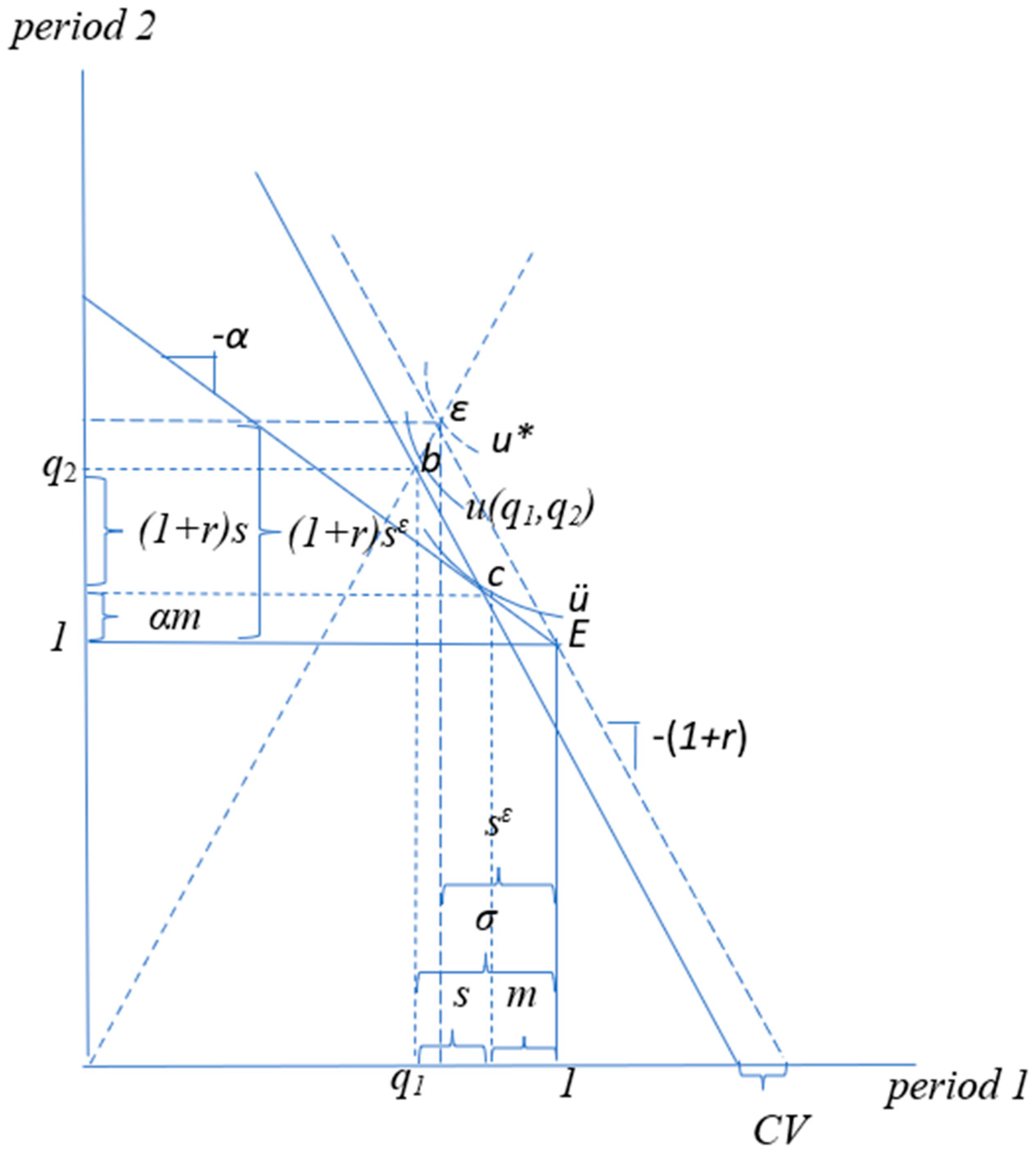
Figure 2.
Life-cycle optimization with education and cash insurance.
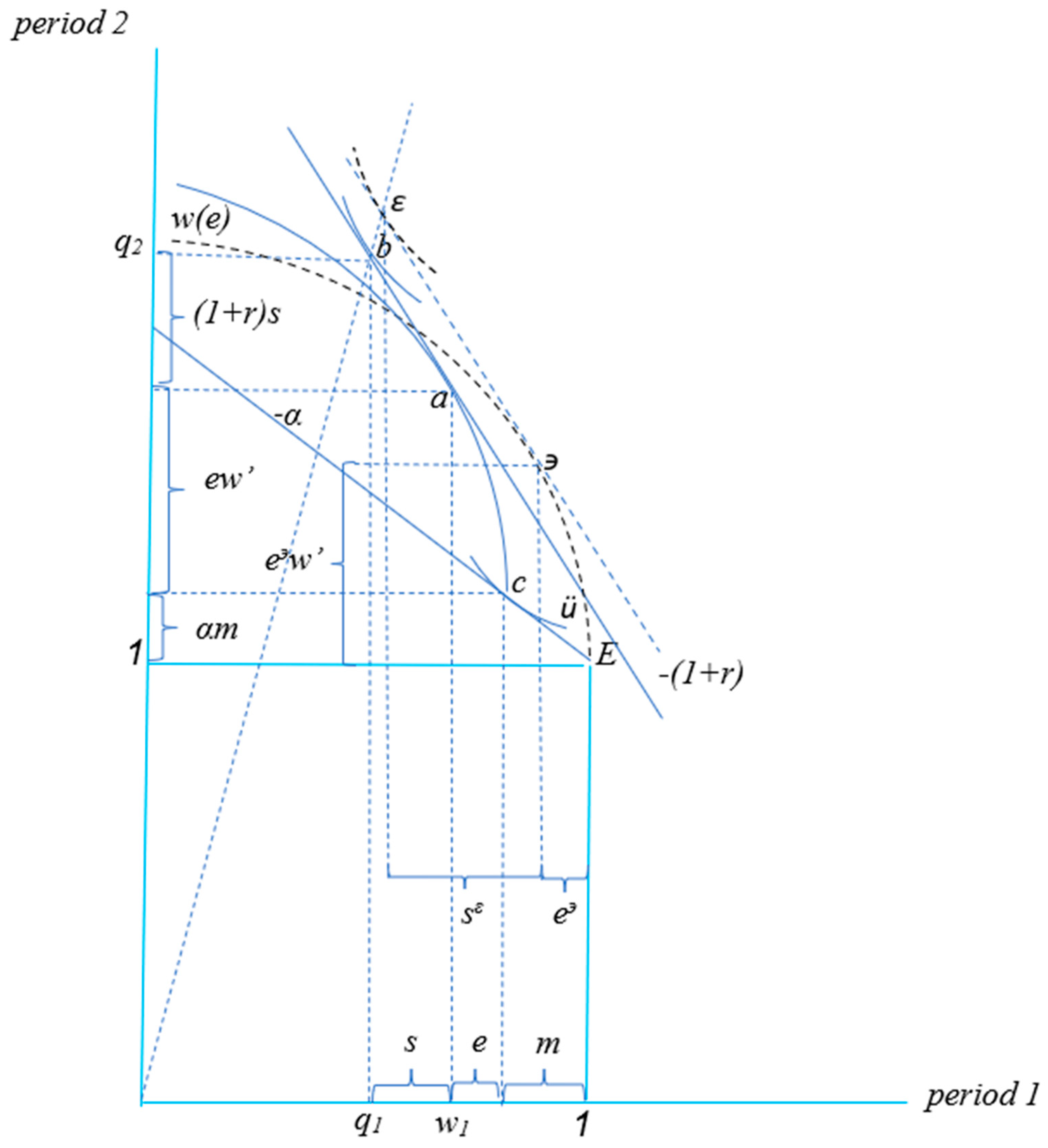
Figure 3.
Absolute money illusion in the life-cycle model.

Publisher’s Note: MDPI stays neutral with regard to jurisdictional claims in published maps and institutional affiliations. |
© 2022 by the author. Licensee MDPI, Basel, Switzerland. This article is an open access article distributed under the terms and conditions of the Creative Commons Attribution (CC BY) license (https://creativecommons.org/licenses/by/4.0/).
Share and Cite
MDPI and ACS Style
Laurila, H. Money as Insurance. Risks 2022, 10, 238. https://doi.org/10.3390/risks10120238
AMA Style
Laurila H. Money as Insurance. Risks. 2022; 10(12):238. https://doi.org/10.3390/risks10120238
Chicago/Turabian StyleLaurila, Hannu. 2022. "Money as Insurance" Risks 10, no. 12: 238. https://doi.org/10.3390/risks10120238
APA StyleLaurila, H. (2022). Money as Insurance. Risks, 10(12), 238. https://doi.org/10.3390/risks10120238
Note that from the first issue of 2016, this journal uses article numbers instead of page numbers. See further details here.