
Forecasting Bitcoin Volatility Using Hybrid GARCH Models with Machine Learning


Abstract
1. Introduction
2. Model Specifications
2.1. Volatility Models
2.2. Recurrent Neural Networks
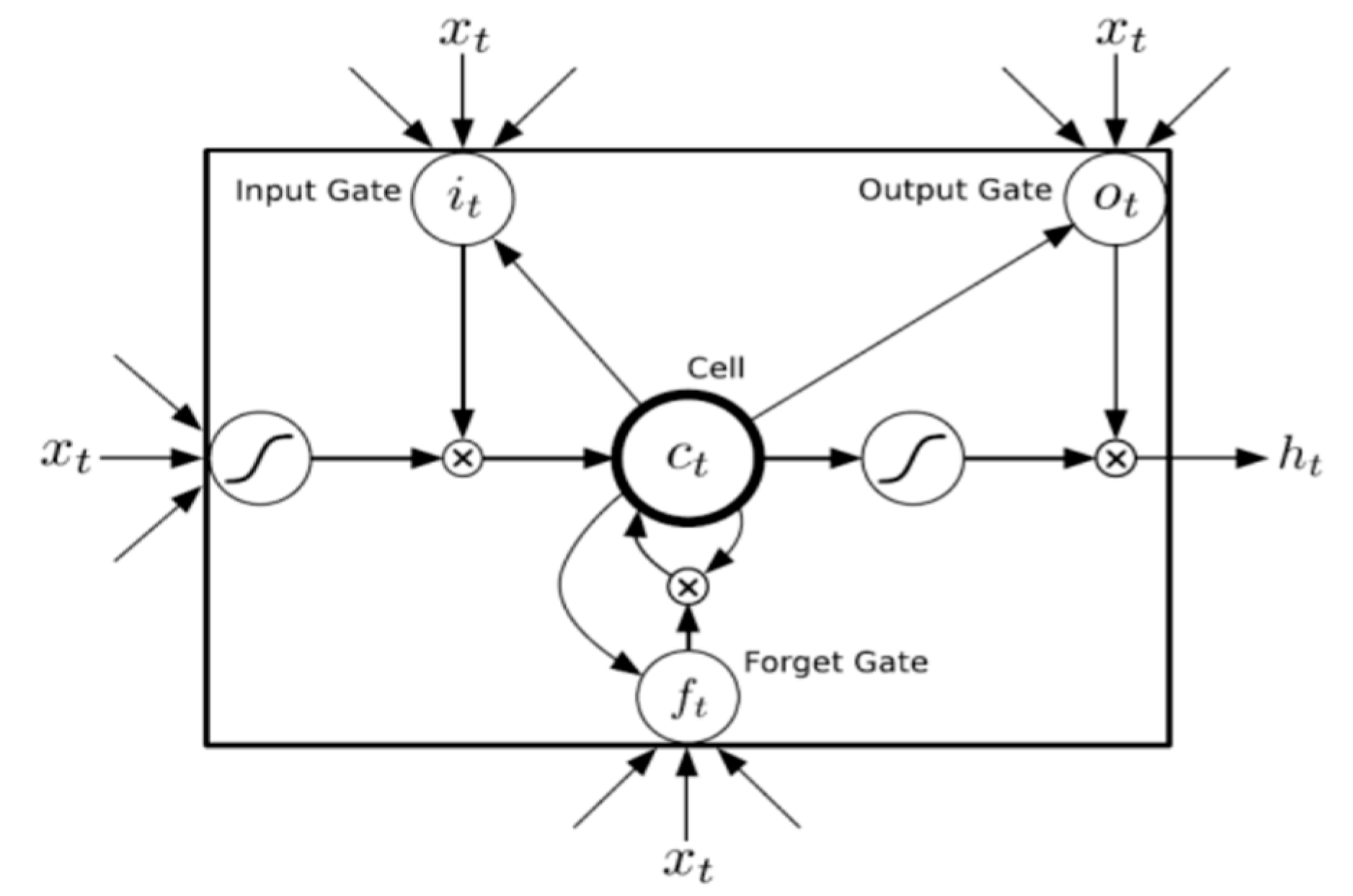
2.3. Long Short-Term Memory
2.4. Gated Recurrent Unit
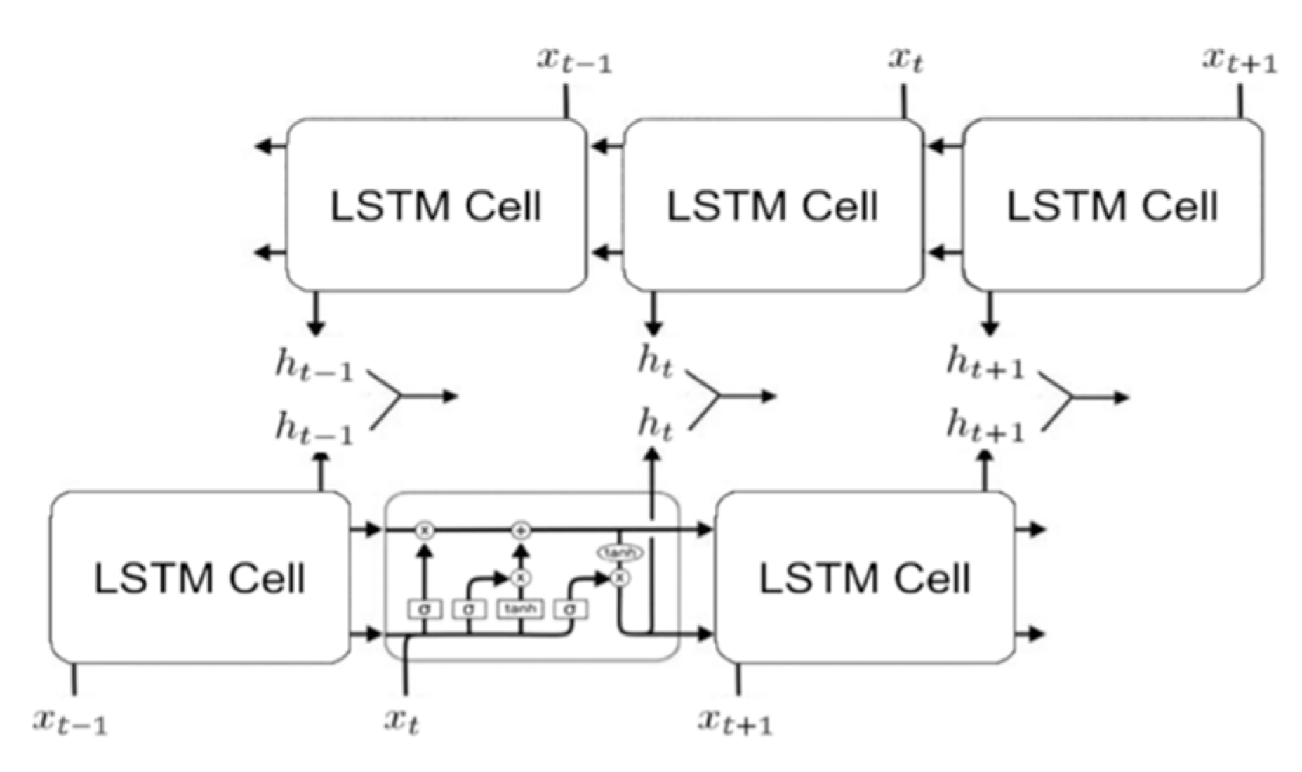
2.5. Bidirectional LSTM
3. Data and Methodology
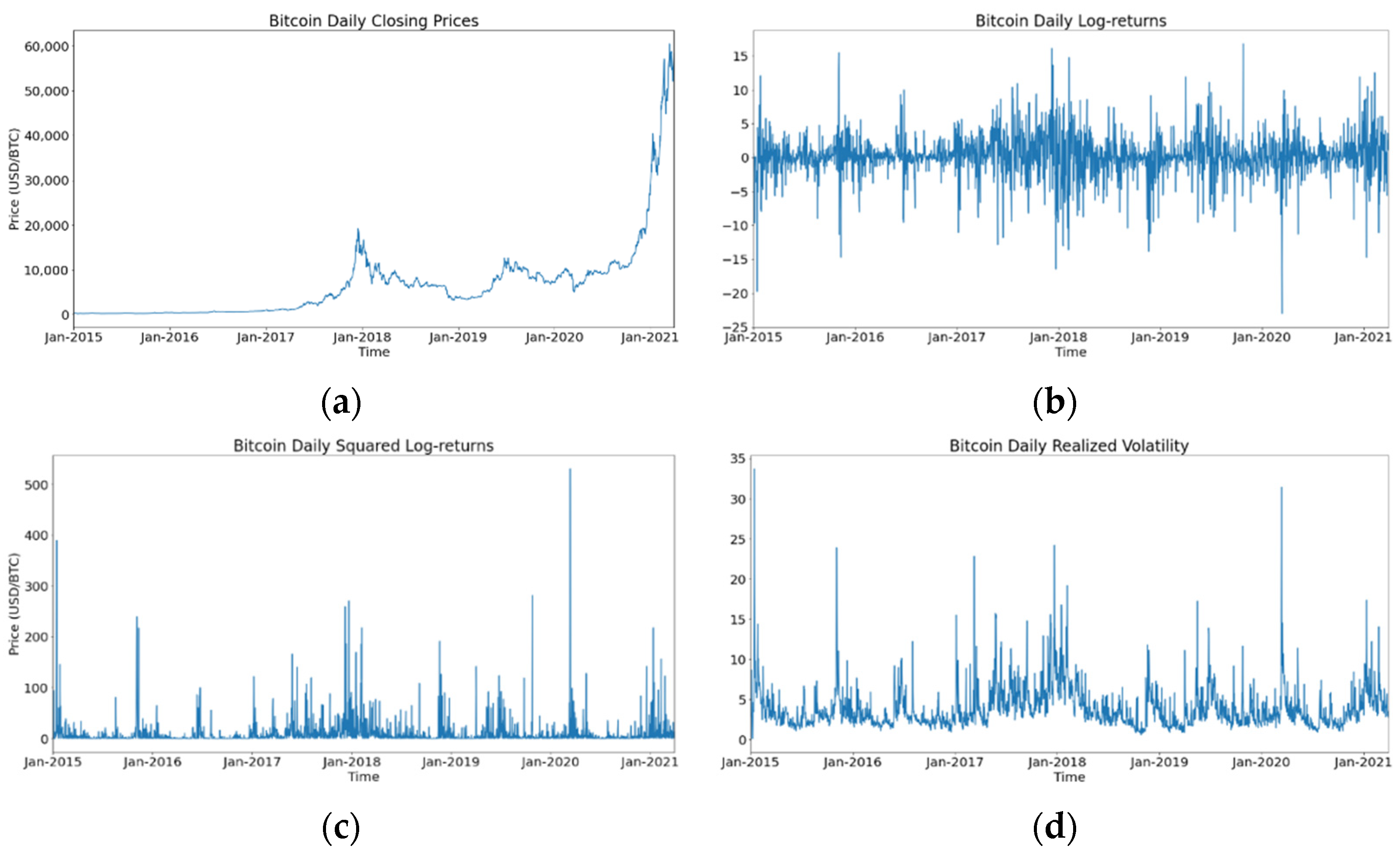
3.1. Data Description
3.2. Evaluation Measures
3.3. Experiments
4. Results and Discussion
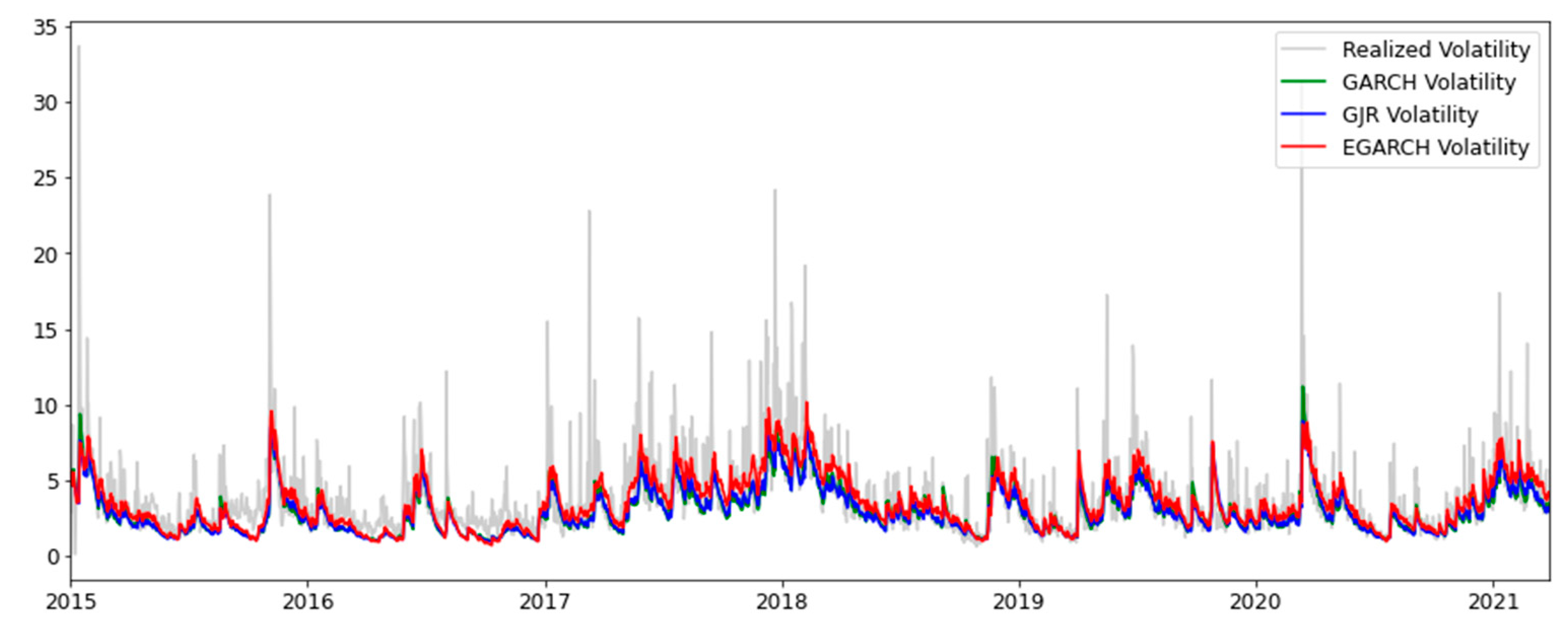
4.1. Estimation Results
4.2. Out-of-Sample Forecast Results
4.3. Rolling Window Forecast Results
5. Concluding Remarks
Author Contributions
Funding
Data Availability Statement
Conflicts of Interest
References
- Al-Yahyaee, Khamis Hamed, Walid Mensi, Idries Mohammad Wanas Al-Jarrah, Atef Hamdi, and Kang Sang Hoon. 2019. Volatility forecasting, downside risk, and diversification benefits of Bitcoin and oil and international commodity markets: A comparative analysis with yellow metal. The North American Journal of Economics and Finance 49: 104–20. [Google Scholar] [CrossRef]
- Aysan, Ahmet Faruk, Asad Ul Islam Khan, and Humeyra Topuz. 2021. Bitcoin and Altcoins Price Dependency: Resilience and Portfolio Allocation in COVID-19 Outbreak. Risks 9: 74. [Google Scholar] [CrossRef]
- Baur, Dirk G., and Thomas Dimpfl. 2018. Asymmetric volatility in cryptocurrencies. Economics Letters 173: 148–51. [Google Scholar] [CrossRef]
- Bollerslev, Tim. 1986. Generalized autoregressive conditional heteroskedasticity. Journal of Econometrics 31: 307–27. [Google Scholar] [CrossRef]
- Bouoiyour, Jamal, and Refk Selmi. 2016. Bitcoin: A beginning of a new phase. Economics Bulletin 36: 1430–40. [Google Scholar]
- Bowden, James, King Timothy, Dimitrios Koutmos, Tiago Loncan, and Francesco Saverio Stentella Lopes Stentella. 2021. A Taxonomy of FinTech Innovation. In Disruptive Technology in Banking and Finance. London: Palgrave Macmillan, pp. 47–91. [Google Scholar]
- Butner, Johnatan E., Ascher K. Munion, Brian R. W. Baucom, and Alexander Wong. 2019. Ghost hunting in the nonlinear dynamic machine. PLoS ONE 14: e0226572. [Google Scholar] [CrossRef]
- Charles, Amélie, and Olivier Darné. 2019. Volatility estimation for Bitcoin: Replication and robustness. International Economics 157: 23–32. [Google Scholar] [CrossRef]
- Cho, Kyunghyun, Bart Van Merrienboer, Caglar Gulcehre, Dzmitry Bahdanau, Fethi Bougares, Holger Schwenk, and Yoshua Bengio. 2014. Learning phrase representations using RNN encoder-decoder for statistical machine translation. Paper presented at 2014 Conference on Empirical Methods in Natural Language Processing (EMNLP), Doha, Qatar, October 26–28; Stroudsburg: Association for Computational Linguistics, pp. 1724–34. [Google Scholar]
- Chu, Jeffrey, Stephen Chan, Saralees Nadarajah, and Joerg Osterrieder. 2017. GARCH Modelling of Cryptocurrencies. Journal of Risk and Financial Management 10: 17. [Google Scholar] [CrossRef]
- Conrad, Christian, Anessa Custovic, and Eric Ghysels. 2018. Long- and Short-Term Cryptocurrency Volatility Components: A GARCH-MIDAS Analysis. Journal of Risk and Financial Management 11: 23. [Google Scholar] [CrossRef]
- Fang, Fan, Carmine Ventre, Michail Basios, Leslie Kanthan, David Martinez-Rego, Fan Wu, and Lingbo Li. 2022. Cryptocurrency trading: A comprehensive survey. Financial Innovation 8: 1–59. [Google Scholar] [CrossRef]
- Feuerriegel, Stefan, and Ralph Fehrer. 2016. Improving decision analytics with deep learning: The case of financial disclosures. Paper presented at 24th European Conference on Information Systems, Istanbul, Turkey, June 12–15, vol. I, pp. 1–10. [Google Scholar]
- Fuertes, Aana-Maria, Marwan Izzeldin, and Elena Kalotychou. 2009. On forecasting daily stock volatility: The role of intraday information and market conditions. International Journal of Forecasting 25: 259–81. [Google Scholar] [CrossRef]
- Gbadebo, Adedeji D., Ahmed O. Adekunle, Adedokun Wole, Adebayo-Oke A. Lukman, and Joseph Akande. 2021. BTC price volatility: Fundamentals versus information. Cogent Business & Management 8: 1. [Google Scholar] [CrossRef]
- Glosten, Lawrence R., Ravi Jagannathan, and David E. Runkle. 1993. On the relation between the expected value and the volatility of the nominal excess return on stocks. The Journal of Finance 48: 1779–801. [Google Scholar] [CrossRef]
- Graves, Alex, and Jurgen Schmidhuber. 2005. Framewise phoneme classification with bidirectional LSTM and other neural network architectures. Neural Networks 18: 602–10. [Google Scholar] [CrossRef] [PubMed]
- Gyamerah, Samuel A. 2019. Modelling the volatility of Bitcoin returns using GARCH models. Quantitative Finance and Economics 3: 739–53. [Google Scholar] [CrossRef]
- Hinton, Geoffrey Everest, and Ruslan Salakhutdinov. 2006. Reducing the dimensionality of data with neural networks. Science 313: 504–07. [Google Scholar] [CrossRef]
- Hochreiter, Sepp, and Jurgen Schmidhuber. 1997. Long short-term memory. Neural Computation 9: 1735–80. [Google Scholar] [CrossRef]
- Hu, Yan, Jian Ni, and Liu Wen. 2020. A hybrid deep learning approach by integrating LSTM-ANN networks with GARCH model for copper price volatility prediction. Physica A: Statistical Mechanics and its Applications 557: 124907. [Google Scholar] [CrossRef]
- Jeenanunta, Chawalit, Rujira Chaysiri, and Laksmey Thong. 2018. Stock price prediction with long short-term memory recurrent neural network. Paper presented at 2018 International Conference on Embedded Systems and Intelligent Technology & International Conference on Information and Communication Technology for Embedded Systems (ICESIT-ICICTES), Khon Kaen, Thailand, May 7–9; pp. 1–7. [Google Scholar]
- Kamnitsas, Konstantinos, Christian Ledig, Virginia F. J. Newcombe, Joanna P. Simpson, Andrew D. Kane, David K. Menon, and Ben Glocker. 2017. Efficient multi-scale 3D CNN with fully connected CRF for accurate brain lesion segmentation. Medical Image Analysis 36: 61–78. [Google Scholar] [CrossRef]
- Katsiampa, Paraskevi. 2017. Volatility estimation for Bitcoin: A comparison of GARCH models. Economics Letters 158: 3–6. [Google Scholar] [CrossRef]
- Kim, Ha Y., and Chang H. Won. 2018. Forecasting the volatility of stock price index: A hybrid model integrating LSTM with multiple GARCH-type models. Expert Systems with Applications 103: 25–37. [Google Scholar] [CrossRef]
- King, Timothy, Dimitrios Koutmos, and F. S. Stentella Lopes. 2021. Cryptocurrency Mining Protocols: A Regulatory and Technological Overview. In Disruptive Technology in Banking and Finance. London: Palgrave Macmillan, pp. 93–134. [Google Scholar] [CrossRef]
- Koutmos, Dimitrios. 2015. Is there a positive risk-return tradeoff? A forward-looking approach to measuring the equity premium. European Financial Management 21: 974–1013. [Google Scholar] [CrossRef]
- Koutmos, Dimitrios. 2022. Investor sentiment and bitcoin prices. Review of Quantitative Finance and Accounting, 1–29. [Google Scholar] [CrossRef]
- Kraus, Mathias, and Stefan Feuerriegel. 2017. Decision support from financial disclosures with deep neural networks and transfer learning. Decision Support Systems 104: 38–48. [Google Scholar] [CrossRef]
- Kristjanpoller, Warner D., and Esteban Hernández. 2017. Volatility of main metals forecasted by a hybrid ANN-GARCH model with regressors. Expert Systems with Applications 84: 290–300. [Google Scholar] [CrossRef]
- Kristjanpoller, Warner D., and Marcel C. Minutolo. 2016. Forecasting volatility of oil price using an artificial neural network-GARCH model. Expert Systems with Applications 65: 233–41. [Google Scholar] [CrossRef]
- Kristjanpoller, Warner D., and Marcel C. Minutolo. 2018. A hybrid volatility forecasting framework integrating GARCH, artificial neural network, technical analysis and principal components analysis. Expert Systems with Applications 109: 1–11. [Google Scholar] [CrossRef]
- Kyriazis, Nikolaos A. 2021. A Survey on Volatility Fluctuations in the Decentralized Cryptocurrency Financial Assets. Journal of Risk and Financial Management 14: 293. [Google Scholar] [CrossRef]
- Lahmiri, Salim, and Stelios Bekiros. 2019. Cryptocurrency forecasting with deep learning chaotic neural networks. Chaos, Solitons & Fractals 118: 35–40. [Google Scholar]
- Laily, Vania O. N., Budi Warsito, and I. M. Di Asih. 2018. Comparison of ARCH/GARCH model and Elman Recurrent Neural Network on data return of closing price stock. Journal of Physics: Conference Series 1025: 1–12. [Google Scholar]
- Lim, Ching M., and Siok K. Sek. 2013. Comparing the performances of GARCH-type models in capturing the stock market volatility in Malaysia. Procedia Economics and Finance 5: 478–87. [Google Scholar] [CrossRef]
- Makinen, Ymir, Juho Kanniainen, Moncef Gabbouj, and Alexandros Iosifidis. 2019. Forecasting jump arrivals in stock prices: New attention-based network architecture using limit order book data. Quantitative Finance 19: 2033–50. [Google Scholar] [CrossRef]
- Makridakis, Spyros, Evangelos Spiliotis, and Vassilios Assimakopoulos. 2018. Statistical and Machine Learning forecasting methods: Concerns and ways forward. PLoS ONE 13: e0194889. [Google Scholar] [CrossRef] [PubMed]
- Mehtab, Sidra, Jaydip Sen, and Abhishek Dutta. 2020. Stock price prediction using machine learning and LSTM-based deep learning models. In Symposium on Machine Learning and Metaheuristics Algorithms, and Applications. Singapore: Springer, pp. 88–106. [Google Scholar] [CrossRef]
- Moghar, Adil, and Mhamed Hamiche. 2020. Stock market prediction using LSTM recurrent neural network. Procedia Computer Science 170: 1168–73. [Google Scholar] [CrossRef]
- Muhammed, Garzali, and Bashir U. Faruk. 2018. The relevance of GARCH-family models in forecasting Nigerian oil price volatility. Central Bank of Nigeria Bullion 42: 14–30. [Google Scholar]
- Naimy, Viviane, Omar Haddad, Gema Fernández-Avilés, and Rim El Khoury. 2021. The predictive capacity of GARCH-type models in measuring the volatility of crypto and world currencies. PLoS ONE 16: e0245904. [Google Scholar] [CrossRef]
- Nelson, Daniel B. 1991. Conditional heteroskedasticity in asset returns: A new approach. Econometrica: Journal of the Econometric Society 59: 347–70. [Google Scholar] [CrossRef]
- Pabuçcu, Hakan, Ongan Serdar, and Ayse Ongan. 2020. Forecasting the movements of Bitcoin prices: An application of machine learning algorithms. Quantitative Finance and Economics 4: 679–92. [Google Scholar] [CrossRef]
- Peng, Yaohoa, Pedro Henrique Melo Albuquerque, Jader Martins Camboim de Sá, Ana Julia Akaishi Padula, and Mariana R. Montenegro. 2018. The best of two worlds: Forecasting high frequency volatility for cryptocurrencies and traditional currencies with Support Vector Regression. Expert Systems with Applications 97: 177–92. [Google Scholar] [CrossRef]
- Phillip, Andrew, Jennifer S. K. Chan, and Shelton Peiris. 2020. A new look at cryptocurrencies. Economics Letters 16: 6–9. [Google Scholar] [CrossRef]
- Qiu, Jiayu, Bin Wang, and Changjun Zhou. 2020. Forecasting stock prices with long-short term memory neural network based on attention mechanism. PLoS ONE 15: e0227222. [Google Scholar] [CrossRef] [PubMed]
- Schuster, Mike, and Kuldip K. Paliwal. 1997. Bidirectional recurrent neural networks. IEEE Transactions on Signal Processing 45: 2673–81. [Google Scholar] [CrossRef]
- Seo, Monghwan, and Geonwoo Kim. 2020. Hybrid Forecasting Models Based on the Neural Networks for the Volatility of Bitcoin. Applied Sciences 10: 4768. [Google Scholar] [CrossRef]
- Shang, Han L., and Steven Haberman. 2018. Model confidence sets and forecast combination: An application to age-specific mortality. Genus 74: 1–23. [Google Scholar] [CrossRef] [PubMed]
- Shen, Ze, Qing Wan, and David J. Leatham. 2021. Bitcoin Return Volatility Forecasting: A Comparative Study between GARCH and RNN. Journal of Risk and Financial Management 14: 337. [Google Scholar] [CrossRef]
- Siegelmann, Hava T., and Eduardo D. Sontag. 1991. Turing computability with neural nets. Applied Mathematics Letters 4: 77–80. [Google Scholar] [CrossRef]
- Sim, Hyun S., Hae I. Kim, and Jae J. Ahn. 2019. Is deep learning for image recognition applicable to stock market prediction? Complexity 2019: 4324878. [Google Scholar] [CrossRef]
- Singh, Ritika, and Shashi Srivastava. 2017. Stock prediction using deep learning. Multimedia Tools and Applications 76: 18569–84. [Google Scholar] [CrossRef]
- Struga, Kejsi, and Olti Qirici. 2018. Bitcoin Price Prediction with Neural Networks. Paper presented at the the 3rd International Conference on Recent Trends and Applications in Computer Science and Information Technology (RTA-CSIT), Tirana, Albania, May 21–22; pp. 41–49. Available online: https://www.semanticscholar.org/paper/Bitcoin-Price-Prediction-with-Neural-Networks-Struga-Qirici/78227a1267464c132236b0bf25a0db812788b864 (accessed on 1 January 2022).
- Verma, Sauraj. 2021. Forecasting volatility of crude oil futures using a GARCH–RNN hybrid approach. Intelligent Systems in Accounting, Finance and Management 28: 130–42. [Google Scholar] [CrossRef]
- Vidal, Andres, and Werner Kristjanpoller. 2020. Gold volatility prediction using a CNN-LSTM approach. Expert Systems with Applications 157: 113481. [Google Scholar] [CrossRef]
- Vo, Nhi N. Y., Xue-Zhong He, Shaowu Liu, and Guandong Xu. 2019. Deep learning for decision making and the optimization of socially responsible investments and portfolio. Decision Support Systems 124: 113097. [Google Scholar] [CrossRef]
- Wellenreuther, Claudia, and Jan Voelzke. 2019. Speculation and volatility A time-varying approach applied on Chinese commodity futures markets. Journal of Futures Markets 39: 405–17. [Google Scholar] [CrossRef]
- Zahid, Mamoona, Farhat Iqbal, Abdul Raziq, and Naveed Sheikh. 2022. Modeling and Forecasting the Realized Volatility of Bitcoin using Realized HAR-GARCH-type Models with Jumps and Inverse Leverage Effect. Sains Malaysiana 51: 929–42. [Google Scholar] [CrossRef]
- Zhang, Zihao, Stefan Zohren, and Stephen Roberts. 2019. Deeplob: Deep convolutional neural networks for limit order books. IEEE Transactions on Signal Processing 67: 3001–12. [Google Scholar] [CrossRef]


| Mean | Std. Dev. | Skewness | Kurtosis | JB | ADF | ARCH(12) | (20) | |
|---|---|---|---|---|---|---|---|---|
| Bitcoin closing prices | 6698.595 | 9279.506 | 3.290 | 13.017 | 20,227.478 | −4.897 | 243.488 *** | 38,493.172 *** |
| RSI | 55.674 | 16.669 | 0.072 | −0.4301 | 19.576 | −6.936 | 2107.303 *** | 17,499.154 *** |
| RVI | 55.908 | 15.739 | 0.053 | −0.073 | 1.590 | −8.594 | 1763.135 *** | 8421.058 *** |
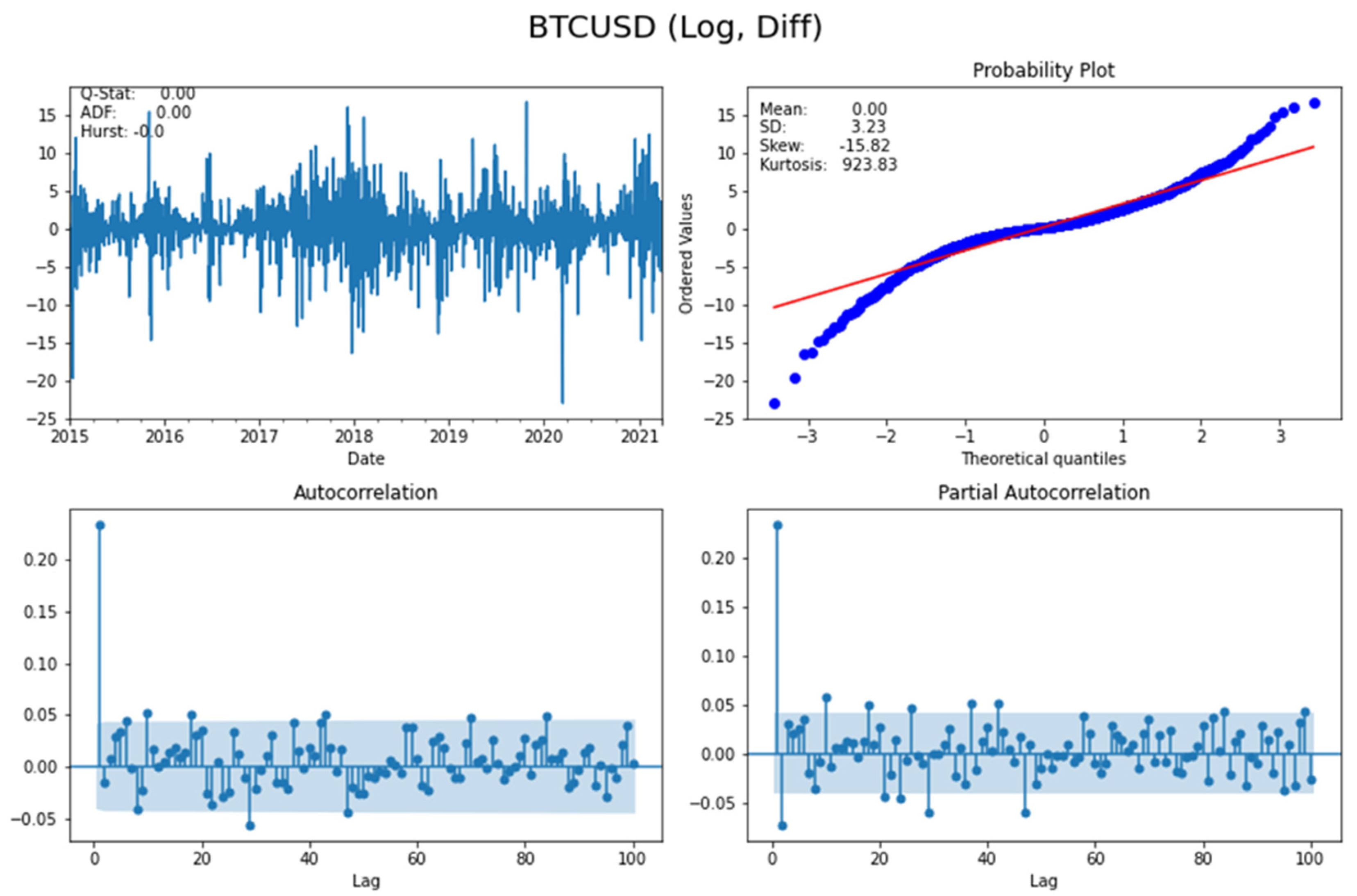
| Bitcoin log-returns | 0.00 4 | 3.229 | 15.820 | 923.830 | 2968.189 | −31.786 | 243.488 *** | 159.362 *** |
| Bitcoin squared log-returns | 10.472 | 28.344 | 7.441 | 85.787 | 720,809.075 | −6.713 | 86.503 *** | 512.371 *** |
| Model | ||||
|---|---|---|---|---|
| GARCH(1,1) | 0.1347 *** (0.008) | 0.1758 *** (0.0003) | – | 0.8242 *** (0.0004) |
| GJR(1,1) | 0.1150 *** (0.0008) | 0.1907 *** (0.0004) | −0.0511 *** (0.0003) | 0.8340 *** (0.0005) |
| EGARCH(1,1) | 0.1083 *** (0.0004) | 0.3744 *** (0.0008) | 0.0245 *** (0.0002) | 0.9824 *** (0.0001) |
| 7-Day-Ahead Forecast | 14-Day-Ahead Forecast | 21-Day-Ahead Forecast | ||||
|---|---|---|---|---|---|---|
| Models | HMAE | HMSE | HMAE | HMSE | HMAE | HMSE |
| GARCH | 0.40406 | 0.40106 | 0.40857 | 0.39108 | 0.41220 | 0.40008 |
| GJR | 0.40445 | 0.39999 | 0.40657 | 0.38999 | 0.41009 | 0.40001 |
| EGARCH | 0.39770 | 0.38956 | 0. 39940 | 0.37999 | 0.40240 | 0.38750 |
| GARCH-LSTM2 | 0.39001 | 0.38001 | 0.38995 | 0.36700 | 0.38995 | 0.37550 |
| GARCH-GRU2 | 0.39450 | 0.38303 | 0.39545 | 0.39303 | 0.41692 | 0.39663 |
| GARCH-BiLSTM2 | 0.39455 | 0.38362 | 0.39551 | 0.39463 | 0.42082 | 0.39620 |
| GJR-LSTM2 | 0.38794 | 0.37699 | 0.38798 | 0.36720 | 0.38991 | 0.37340 |
| GJR-GRU2 | 0.39650 | 0.38079 | 0.39740 | 0.39977 | 0.39920 | 0.37998 |
| GJR-BiLSTM2 | 0.39555 | 0.38270 | 0.39605 | 0.39621 | 0.41805 | 0. 38721 |
| EGARCH-LSTM2 | 0.37998 | 0.36799 | 0.37999 | 0.35800 | 0.37991 | 0.36400 |
| EGARCH-GRU2 | 0.39705 | 0.38354 | 0.39905 | 0.37655 | 0.40002 | 0.38632 |
| EGARCH-BiLSTM2 | 0.39736 | 0.38680 | 0.39740 | 0.38759 | 0.39748 | 0.38498 |
| 7 Days Ahead Forecast | 14 Days Ahead Forecast | 21 Days Ahead Forecast | ||||
|---|---|---|---|---|---|---|
| Models | HMAE | HMSE | HMAE | HMSE | HMAE | HMSE |
| GARCH-GJR-LSTM2 | 0.35505 | 0.33935 | 0.35400 | 0.32940 | 0.35301 | 0.33440 |
| GARCH-GJR-GRU2 | 0.37876 | 0.33511 | 0.37881 | 0.33447 | 0.37901 | 0.33373 |
| GARCH-GJR-BiLSTM1 | 0.37801 | 0.34511 | 0.37825 | 0.34541 | 0.37900 | 0.34722 |
| GARCH-EGARCH-LSTM2 | 0.34601 | 0.33250 | 0.34440 | 0.32150 | 0.34240 | 0.32650 |
| GARCH-EGARCH-GRU2 | 0.37581 | 0.34303 | 0.37602 | 0.34325 | 0.37102 | 0.34563 |
| GARCH-EGARCH-BiLSTM1 | 0.37660 | 0.35505 | 0.37851 | 0.35461 | 0.37952 | 0.35561 |
| GJR-EGARCH-LSTM2 | 0.35105 | 0.33835 | 0.35100 | 0.32740 | 0.35001 | 0.33240 |
| GJR-EGARCH- GRU2 | 0.37400 | 0.33851 | 0.37756 | 0.33457 | 0.41373 | 0.33650 |
| GJR-EGARCH-BiLSTM1 | 0.37410 | 0.33789 | 0.33889 | 0.33889 | 0.38405 | 0.33884 |
| GARCH-GJR-EGARCH-LSTM2 | 0.33280 | 0.30281 | 0.33282 | 0.30110 | 0.32002 | 0.30020 |
| GARCH-GJR-EGARCH-GRU2 | 0.34325 | 0.30380 | 0.35914 | 0.30604 | 0.35942 | 0.30098 |
| GARCH-GJR-EGARCH-BiLSTM2 | 0.33809 | 0.30381 | 0.34250 | 0.30241 | 0.35010 | 0.30491 |
| One Day Rolling Window at 7 Days Ahead Forecast | One Day Rolling Window at 14 Days Ahead Forecast | One Day Rolling Window at 21 Days Ahead Forecast | ||||
|---|---|---|---|---|---|---|
| Models | HMAE | HMSE | HMAE | HMSE | HMAE | HMSE |
| GARCH-LSTM2 | 0.38890 | 0.38761 | 0.38892 | 0.38265 | 0.38895 | 0.37650 |
| GARCH-GRU2 | 0.39120 | 0.38000 | 0.39122 | 0.38102 | 0.39105 | 0.38202 |
| GARCH-BiLSTM1 | 0.39155 | 0.39263 | 0.39255 | 0.39264 | 0.39355 | 0.38421 |
| GJR-LSTM2 | 0.38120 | 0.36604 | 0.38122 | 0.36702 | 0.38225 | 0.36851 |
| GJR-GRU3 | 0.38704 | 0.37079 | 0.38854 | 0.37178 | 0.38902 | 0.37256 |
| GJR-BiLSTM2 | 0.38777 | 0.37217 | 0.38901 | 0.37122 | 0.38906 | 0.37522 |
| EGARCH-LSTM2 | 0.37707 | 0.35561 | 0.35720 | 0.33650 | 0.35299 | 0.33602 |
| EGARCH-GRU2 | 0.38706 | 0.36455 | 0.38746 | 0.36456 | 0.38801 | 0.38298 |
| EGARCH-BiLSTM2 | 0.38737. | 0.38381 | 0.38740 | 0.38385 | 0.38902 | 0.38386 |
| One Day Rolling Window at 7 Days Ahead Forecast | One Day Rolling Window at 14 Days Ahead Forecast | One Day Rolling Window at 21 Days Ahead Forecast | ||||
|---|---|---|---|---|---|---|
| Models | HMAE | HMSE | HMAE | HMSE | HMAE | HMSE |
| GARCH-GJR-LSTM2 | 0.37430 | 0.29930 | 0.37200 | 0.28454 | 0.37250 | 0.28484 |
| GARCH-GJR-GRU2 | 0.37680 | 0.30210 | 0.37680 | 0.30247 | 0.37701 | 0. 30373 |
| GARCH-GJR-BiLSTM1 | 0.37600 | 0.29790 | 0.37620 | 0.30021 | 0.37700 | 0.30122 |
| GARCH-EGARCH-LSTM | 0.34000 | 0.29857 | 0.31540 | 0.28125 | 0.31250 | 0.27527 |
| GARCH-EGARCH-GRU2 | 0.37380 | 0.29420 | 0.37400 | 0.30000 | 0.37102 | 0.30025 |
| GARCH-EGARCH-BiLSTM2 | 0.37460 | 0.29300 | 0.37750 | 0.29261 | 0.37752 | 0.29361 |
| GJR-EGARCH- LSTM2 | 0.37460 | 0.29450 | 0.37650 | 0.28454 | 0.37752 | 0.27650 |
| GJR-EGARCH- GRU2 | 0.37200 | 0.29650 | 0.377360 | 0.28257 | 0.41173 | 0.28180 |
| GJR-EGARCH-BiLSTM1 | 0.37210 | 0.29790 | 0.37220 | 0.30005 | 0.38205 | 0.30084 |
| GARCH-GJR-EGARCH-LSTM2 | 0.29085 | 0.25000 | 0.26921 | 0.23201 | 0.26580 | 0.22205 |
| GARCH-GJR-EGARCH-GRU2 | 0.33180 | 0.27000 | 0.29124 | 0.23301 | 0.24004 | 0.23101 |
| GARCH-GJR-EGARCH-BiLSTM2 | 0.30610 | 0.27080 | 0.30650 | 0.27141 | 0.30810 | 0.26991 |
| Hybrid Models. | Days Ahead Forecast | HMAE | HMSE | Significance |
|---|---|---|---|---|
| EGARCH-LSTM2 | 7 | 0.37707 | 0.35561 | ** |
| 14 | 0.35920 | 0.33650 | ** | |
| 21 | 0.35299 | 0.33602 | * | |
| GARCH-EGARCH-LSTM2 | 7 | 0.34000 | 0.29857 | * |
| 14 | 0.31540 | 0.28125 | ** | |
| 21 | 0.31250 | 0.27527 | * | |
| GARCH-GJR-EGARCH LSTM2 | 7 | 0.29805 | 0.25000 | ** |
| 14 | 0.26921 | 0.23201 | *** | |
| 21 | 0.26580 | 0.22205 | * | |
| GARCH-GJR-EGARCH-GRU2 | 7 | 0.30180 | 0.27000 | ** |
| 14 | 0.29124 | 0.23301 | ** | |
| 21 | 0.29008 | 0.23301 | ** | |
| GARCH-GJR-EGARCH-BiLSTM2 | 7 | 0.30610 | 0.27080 | ** |
| 14 | 0.30650 | 0.27141 | * | |
| 21 | 0.30810 | 0.27290 | ** |
Publisher’s Note: MDPI stays neutral with regard to jurisdictional claims in published maps and institutional affiliations. |
© 2022 by the authors. Licensee MDPI, Basel, Switzerland. This article is an open access article distributed under the terms and conditions of the Creative Commons Attribution (CC BY) license (https://creativecommons.org/licenses/by/4.0/).
Share and Cite
Zahid, M.; Iqbal, F.; Koutmos, D. Forecasting Bitcoin Volatility Using Hybrid GARCH Models with Machine Learning. Risks 2022, 10, 237. https://doi.org/10.3390/risks10120237
Zahid M, Iqbal F, Koutmos D. Forecasting Bitcoin Volatility Using Hybrid GARCH Models with Machine Learning. Risks. 2022; 10(12):237. https://doi.org/10.3390/risks10120237
Chicago/Turabian StyleZahid, Mamoona, Farhat Iqbal, and Dimitrios Koutmos. 2022. "Forecasting Bitcoin Volatility Using Hybrid GARCH Models with Machine Learning" Risks 10, no. 12: 237. https://doi.org/10.3390/risks10120237
APA StyleZahid, M., Iqbal, F., & Koutmos, D. (2022). Forecasting Bitcoin Volatility Using Hybrid GARCH Models with Machine Learning. Risks, 10(12), 237. https://doi.org/10.3390/risks10120237