
Spectral Expansions for Credit Risk Modelling with Occupation Times


Abstract
1. Introduction
2. Occupation Time Process for Underlying Diffusion
3. Occupation Time Process for -Diffusion
4. Occupation Time Model in the Risk-Neutral Measure
5. Hazard Rate Model
6. Probability of Default
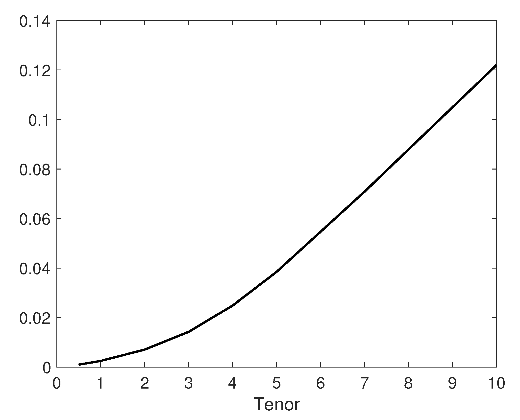
7. Implied Hazard Rate Function
8. Credit Default Swap (CDS) Spreads
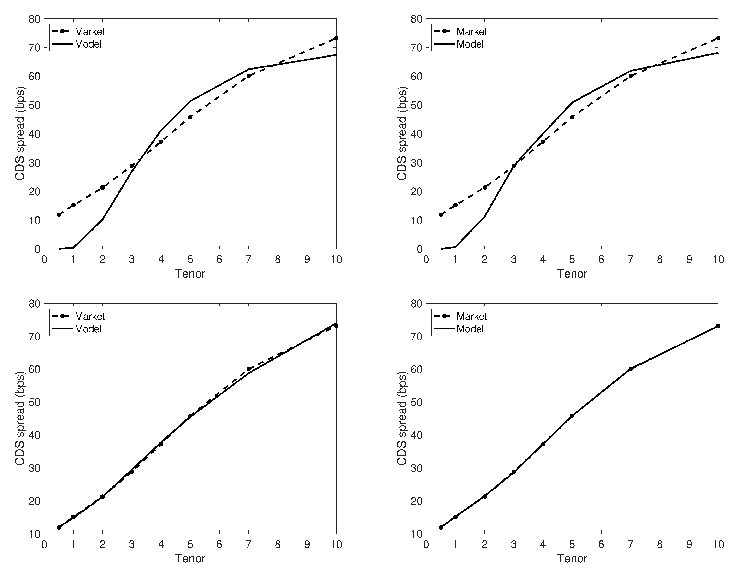
9. Calibration of CDS Spreads: GBM Case
- The Black–Cox model Black and Cox (1976)
- The Alfonsi–Lelong model Alfonsi and Lelong (2012)
- The new hazard rate model (with defined in (48))
10. Conclusions
Author Contributions
Funding
Institutional Review Board Statement
Informed Consent Statement
Data Availability Statement
Conflicts of Interest
Appendix A. Explicit Expressions for a Drifted Brownian Motion
Appendix A.1. Default Probabilities
- If ,
- If ,
- If ,
- If ,
Appendix A.2. CDS Spread
- If ,
- If ,
| 1 | Here we distinguish the X-diffusion from the F-diffusion (i.e., the firm’s value process) which is obtained through a smooth monotonic mapping (where is the state space for the F-diffusion) with unique inverse . |
| 2 | The cemetery state is not included in the interval . When the process is killed and immediately sent to the cemetery state, it stays there indefinitely. |
| 3 | for any random variable X and event A. |
| 4 | |
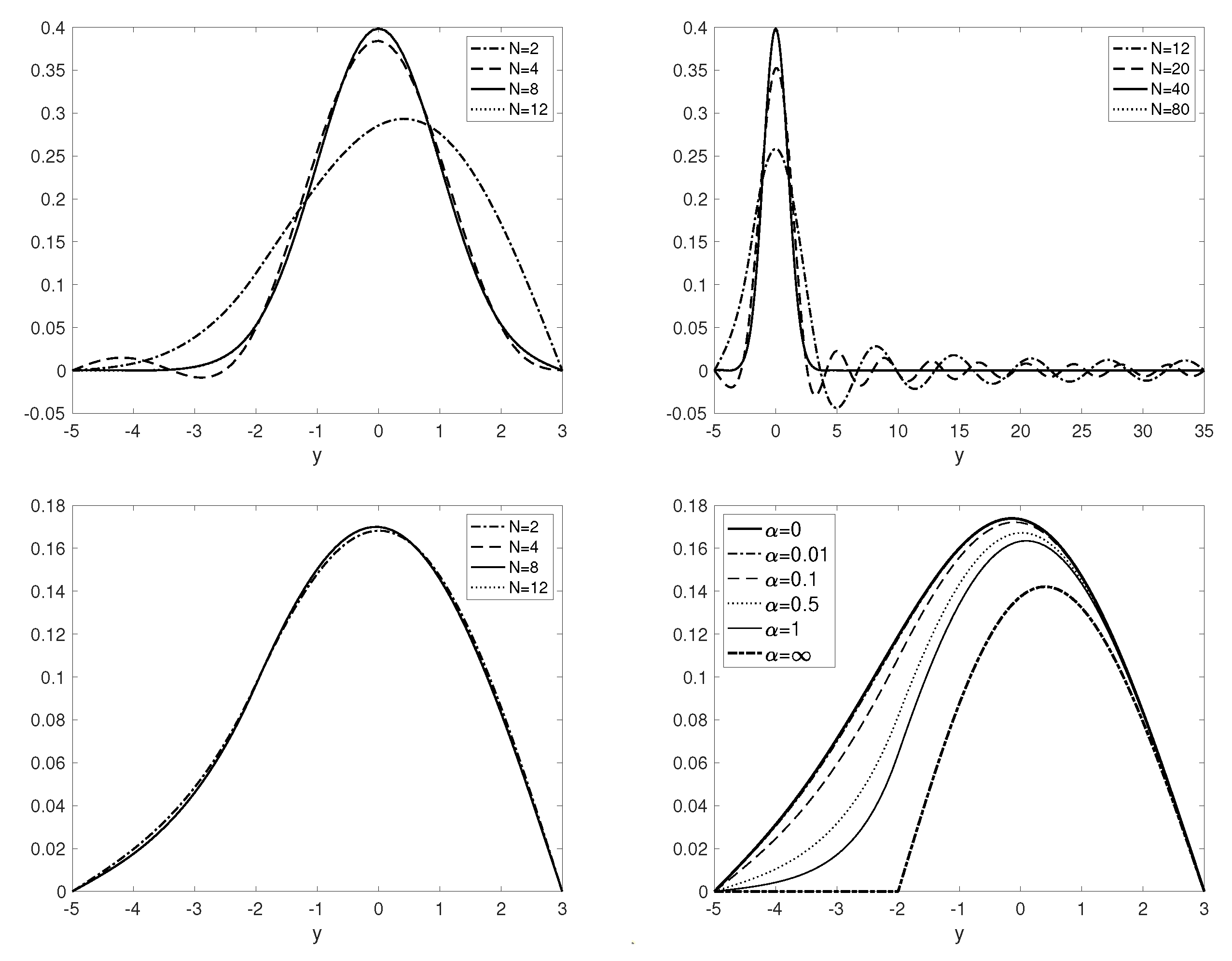
| 5 | When , we obtain the regular transition density of without an instantaneous killing:
|
| 6 | The transition and joint densities are pointwise convergent as :
|
| 7 | We assume there exists a risk-neutral probability equivalent to so that the discounted price process of the defaultable claim is a Doob–Levy -martingale. In the GBM model, we clearly have the discounted firm’s value process , as a -martingale. |
| 8 | . |
| 9 | For , Theorem 1 extends to the time-t value of the credit derivative since , thanks to Lemma 1. |
| 10 | , for , where the T-maturity credit derivative price corresponds to that in the Black–Cox model with default barrier . |
| 11 | The name “hazard rate model” comes from the fact that we are employing a hazard rate process to model default probabilities. |
| 12 | For , Theorem 2 extends to the time-t value of the credit derivative: . |
| 13 | We can easily extend it to the hazard rate model with defined in (48), since
|
| 14 | Under the occupation time model, the implied hazard rate function can be computed by Laplace inverting, with respect to , of the numerator and denominator in (60) separately. |
| 15 | We can easily extend it to the hazard rate model with defined in (48), by sending and . |
| 16 | Under the occupation time model, the implied hazard rate function can be computed by Laplace inverting, with respect to , of and in (64). |
| 17 | The eigenvalues can be obtained numerically by the bisection or Newton-Raphson methods. |
References
- Alfonsi, Aurélien, and Jérôme Lelong. 2012. A closed-form extension to the Black-Cox model. International Journal of Theoretical and Applied Finance 15: 1250053. [Google Scholar] [CrossRef]
- Bielecki, Tomasz R., and Marek Rutkowski. 2013. Credit Risk: Modeling, Valuation and Hedging. Berlin/Heidelberg: Springer. [Google Scholar]
- Black, Fischer, and John C. Cox. 1976. Valuing corporate securities: Some effects of bond indenture provisions. The Journal of Finance 31: 351–67. [Google Scholar] [CrossRef]
- Borodin, Andrei N., and Paavo Salminen. 2002. Handbook of Brownian Motion—Facts and Formulae, 2nd ed. Probability and Its Applications. Basel: Birkhäuser. [Google Scholar]
- Broadie, Mark, Mikhail Chernov, and Suresh Sundaresan. 2007. Optimal debt and equity values in the presence of Chapter 7 and Chapter 11. Journal of Finance 62: 1341–77. [Google Scholar] [CrossRef]
- Campolieti, Giuseppe. Solvable Diffusions in Financial Mathematics. manuscript in preparation, to be published.
- Campolieti, Giuseppe, Roman N. Makarov, and Karl Wouterloot. 2013. Pricing step options under the CEV and other solvable diffusion models. International Journal of Theoretical and Applied Finance 16: 1350027. [Google Scholar] [CrossRef]
- Chesney, Marc, Monique Jeanblanc-Picqué, and Marc Yor. 1997. Brownian excursions and Parisian barrier options. Advances in Applied Probability 29: 165–84. [Google Scholar] [CrossRef]
- Cohen, Alan M. 2007. Numerical Methods for Laplace Transform Inversion. New York: Springer, vol. 5. [Google Scholar]
- Galai, Dan, Alon Raviv, and Zvi Wiener. 2007. Liquidation triggers and the valuation of equity and debt. Journal of Banking and Finance 31: 3604–20. [Google Scholar] [CrossRef]
- Gaver, Donald P., Jr. 1966. Observing stochastic processes, and approximate transform inversion. Operations Research 14: 444–59. [Google Scholar] [CrossRef]
- Haber, Richard J., Phillip J. Schönbucher, and Paul Wilmott. 1999. Pricing Parisan Options. The Journal of Derivatives 6: 71–79. [Google Scholar] [CrossRef]
- Li, Bin, Qihe Tang, Lihe Wang, and Xiaowen Zhou. 2014. Liquidation risk in the presence of Chapters 7 and 11 of the US bankruptcy code. Journal of Financial Engineering 1: 1450023. [Google Scholar] [CrossRef]
- Linetsky, Vadim. 2004. The spectral decomposition of the option value. International Journal of Theoretical and Applied Finance 7: 337–84. [Google Scholar] [CrossRef]
- Makarov, Roman N., Adam Metzler, and Zi Ni. 2015. Modelling default risk with occupation times. Finance Research Letters 13: 54–65. [Google Scholar] [CrossRef]
- Makarov, Roman N. 2016. Modeling liquidation risk with occupation times. International Journal of Financial Engineering 3: 1650028. [Google Scholar] [CrossRef]
- Merton, Robert C. 1974. On the pricing of corporate debt: The risk structure of interest rates. The Journal of finance 29: 449–70. [Google Scholar]
- Moraux, Franck. 2002. Valuing Corporate Liabilities When the Default Threshold Is Not an Absorbing Barrier. Available online: https://www.worldscientific.com/doi/10.1142/9789814759595_0014 (accessed on 12 December 2021).
- Nardon, Martina. 2008. First passage and excursion time models for valuing defaultable bonds: A review with some insights. Frontiers in Finance and Economics 5: 1–25. [Google Scholar]
- Stehfest, Harald. 1970. Algorithm 368: Numerical inversion of Laplace transforms. Communications of the ACM 13: 47–49. [Google Scholar] [CrossRef]


| Variable Name | Description | Value |
|---|---|---|
| initial firm’s value | ||
| constant risk-free rate | ||
| constant volatility | ||
| constant Loss Given Default |
| Tenor | 0.5 | 1 | 2 | 3 | 4 | 5 | 7 | 10 |
| CDS | 11.86 | 15.13 | 21.29 | 28.79 | 37.21 | 45.83 | 60.03 | 73.17 |
| Variable | Description | Black–Cox | Occupation | A–L | Hazard Rate |
|---|---|---|---|---|---|
| default barrier (at time 0) | NA | ||||
| growth rate of barrier | 11.22% | ||||
| occupation barrier (at time 0) | NA | 23.29 | 28.78 | 38.42 | |
| grace period relative to T | NA | 0.2368 | NA | NA | |
| killing rate (above L) | NA | NA | 0.27% | ||
| killing rate (below L) | NA | NA | 3.42% | ||
| loss function value |
Publisher’s Note: MDPI stays neutral with regard to jurisdictional claims in published maps and institutional affiliations. |
© 2022 by the authors. Licensee MDPI, Basel, Switzerland. This article is an open access article distributed under the terms and conditions of the Creative Commons Attribution (CC BY) license (https://creativecommons.org/licenses/by/4.0/).
Share and Cite
Campolieti, G.; Kato, H.; Makarov, R.N. Spectral Expansions for Credit Risk Modelling with Occupation Times. Risks 2022, 10, 228. https://doi.org/10.3390/risks10120228
Campolieti G, Kato H, Makarov RN. Spectral Expansions for Credit Risk Modelling with Occupation Times. Risks. 2022; 10(12):228. https://doi.org/10.3390/risks10120228
Chicago/Turabian StyleCampolieti, Giuseppe, Hiromichi Kato, and Roman N. Makarov. 2022. "Spectral Expansions for Credit Risk Modelling with Occupation Times" Risks 10, no. 12: 228. https://doi.org/10.3390/risks10120228
APA StyleCampolieti, G., Kato, H., & Makarov, R. N. (2022). Spectral Expansions for Credit Risk Modelling with Occupation Times. Risks, 10(12), 228. https://doi.org/10.3390/risks10120228