Article

Calibrating FBSDEs Driven Models in Finance via NNs

by
Luca Di Persio
1,†,
Emanuele Lavagnoli
1,† and
Marco Patacca
2,*,†
1
Department of Computer Science, University of Verona, via Ca’ Vignal 2, 37129 Verona, Italy
2
Department of Economics and Finance, University of Rome Tor Vergata, via Columbia 2, 00133 Rome, Italy
*
Author to whom correspondence should be addressed.
These authors contributed equally to this work.
Risks 2022, 10(12), 227; https://doi.org/10.3390/risks10120227
Submission received: 8 October 2022 / Revised: 10 November 2022 / Accepted: 23 November 2022 / Published: 30 November 2022

Abstract

:
The curse of dimensionality problem refers to a set of troubles arising when dealing with huge amount of data as happens, e.g., applying standard numerical methods to solve partial differential equations related to financial modeling. To overcome the latter issue, we propose a Deep Learning approach to efficiently approximate nonlinear functions characterizing financial models in a high dimension. In particular, we consider solving the Black–Scholes–Barenblatt non-linear stochastic differential equation via a forward-backward neural network, also calibrating the related stochastic volatility model when dealing with European options. The obtained results exhibit accurate approximations of the implied volatility surface. Specifically, our method seems to significantly reduce the neural network’s training time and the approximation error on the test set.

1. Introduction

The curse of dimensionality problem refers to a set of troubles that arise when dealing with big data. Classical methods for solving partial differential equations suffer from this problem, especially in the financial field (Bayer and Stemper 2018; Wang 2006; Weinan et al. 2019). For example, we can think of the non-linear Black–Scholes equation for pricing financial derivatives in which the number of considered underlying assets gives the dimensionality of the Partial Differential Equation (PDE). The latter scenario, from a purely mathematical point of view, typically translates in the need of approximating nonlinear functions in a high dimension. An effective solution can be obtained exploiting a Deep Learning approach, namely using a particular type of Machine Learning (set of) solutions. For the sake of completeness, let us recall that Machine Learning (ML) is the branch of computer science in which mathematical and statistical techniques are used to give computer systems the ability to learn through data. There are two main branches of ML algorithms: Supervised Learning and Unsupervised Learning. The former use labeled datasets while the latter use unlabeled data. The increase of available data in recent years and the need to analyze them, finds in Machine Learning the ideal tool. Indeed, the peculiar features and the change of programming paradigm of the latter, make it the best candidate to solve problems with huge number of data in different fields. For example, computer vision, natural language processing, time series analysis, differential equation. Many papers have been published with the aim of improving theoretical and empirical knowledge; see, among others, Germain et al. (2021); Han (2016) and (Carleo and Troyer 2017). This fame inspires speculations that Deep Learning might hold the key to solving the curse of dimensionality problem.
Neural networks (NNs) are the backbone of deep learning algorithms and their use to solve real-world problems. Indeed, even if their conceptual development can be dated back to several years ago, only during last few years, particularly since powerful hardware became economical affordable, they proved to be concretely and efficiently applied to fruitfully solve complex tasks dealing with huge amount of data. The latter is the case, e.g., of NNs-steered solution to forecast financial scenarios, aggregate energy consumption, social events, etc.
In this paper, we aim at showing how to use NNs toward two financial connected goals: find a solution of a particular non-linear stochastic differential equation (the Black–Scholes–Barenblatt one) via a forward-backward neural network and to calibrate a stochastic volatility model (the Heston model) using a NN-structure for regression. In both cases, we deal with European option-based pricing models. The two goals are strictly connected from a financial point of view, because the first one provides a solution to the option pricing perspective, while the second covers the model calibration task. Even if they seem different from a mathematical point of view, we underline that the specific features of the proposed methodology allow us to solve them with similar Neural Network specification.
The rest of the paper is divided as follows: Section 2 and Section 3 provide an overview of Backward Stochastic Differential Equations (BSDE) and Neural Networks, respectively, while Section 4 is devoted to depicting the link between BSDEs and NNs, to analyze the type of NN that we choose and why we have considered this specific option. In Section 5, we exploit the obtained findings to calibrate the above mentioned rough stochastic volatility model with NN and in Section 6 we show the empirical results. Finally, Section 7 states our conclusions with possible outlooks. Finally, Appendixes Appendix A and Appendix B collect the main notation and definitions respectively.

2. Backward Stochastic Differential Equations

BSDEs were first introduced in Bismut (1973), where the author described them in connection with stochastic control problems. Then, stochastic control cases have been widely investigated during the 1970s by Bismut himself, as well as by, e.g., Bensoussan; Haussmann; and Kushner, particularly under no control on the diffusion coefficient, while Pardoux and Peng gave a full presentation in Mao (1995). Nowadays, the theory of the hedging and pricing of a contingent claim is typically expressed in terms of a linear Backward Stochastic Differential Equation (BSDE) of Ito’s type. Along the latter lines, let us start defining a filtered probability space, endowed with the usual conditions ( Ω , ( F t ) , F , P ) , where the filtration ( F t ) is the one generated by a standard, real-valued, d dimensional, d 1 , Brownian motion W = { W t : t 0 } , defined on Ω . Accordingly, we define a linear BSDE as follows:
d Y t = + f ( t , Y t , Z t ) d t Z t d W t , t [ 0 , T ] Y T = ζ L p ( Ω , F T , P ) ,
or, equivalently,
Y t = ζ + t T f ( s , Y s , Z s ) d s t T Z s d W s .
The solution of (1) is a pair of processes ( Y , Z ) such that Y is continuous and adapted, and Z is predictable and satisfies 0 T | Z s | 2 d s < a.s.
The parameters f and ξ are called standard parameters if:
  • ζ L T 2 ( R d ) , where L T 2 ( R d ) is the space of F t -measurable random variables ξ s.t. E ( | ξ | 2 ) <
  • f ( t , 0 , 0 ) H T 2 ( R d ) t [ 0 , T ] , where H T 2 ( R d ) is the space of predictable process Y s.t. | | Y | | 2 = E ( 0 T | Y t | 2 d t ) < )
  • f is uniformly Lipschitz: there exists L s.t.
    | f ( t , y 1 , z 1 ) f ( t , y 2 , z 2 ) | L ( | y 1 y 2 | + | z 1 z 2 | )
    for any y 1 , y 2 , z 1 , z 2 .
Theorem 1. 
Given the standard parameters, the BSDE (1) has a unique solution ( Y , Z ) in H T 2 ( R d ) × H T 2 ( R d × n ) .
See El Karoui et al. (1997) for the proof.

Forward–Backward Stochastic Differential Equation

As in the previous case, let us start considering a standard probability space ( Ω , F , P ) , and a d-dimensional Brownian motion W = { W t : t 0 } , where { F t } = σ { W S : 0 s t } . Then, we define a Forward–Backward Stochastic Differential Equation (FBSDE), as follows:
X t = x + 0 t b ( s , X s , Y s , Z s ) d s + 0 t σ ( s , X s , Y s ) d W s Y t = g ( X T ) + t T b ^ ( s , X s , Y s , Z s ) d s + t T σ ^ ( s , X s , Y s , Z s ) d W s ,
where the processes X, Y and Z are in R n , R d and R d × n .
Definition 1. 
A triple of stochastic processes ( X , Y , Z ) : [ 0 , T ] × Ω R n × R d × R d × n is called an ordinary adapted solution of FBSDE (2) if it is { F t } -adapted, square integrable and satisfies (2), P -a.s.
We can also rewrite the system of Equation (2) in a pure forward differential form as follows:
d X t = b ( t , X t , Y t , Z t ) d t + σ ( t , X t , Y t ) d W t d Y t = b ^ ( t , X t , Y t , Z t ) d t σ ^ ( t , X t , Y t ) d W t Y T = g ( X T ) , X 0 = x .
also called a stochastic two-point boundary value problem.
In Pardoux and Tang (1999), it is shown how a couple of FBSDEs of (3)-type are connected to:
u t = f ˜ ( t , x , u , D u , D 2 u ) ,
a quasi-linear partial differential equation with terminal condition given by u ( T , x ) = g ( x ) and where u ( t , x ) is the unknown solution. The function f ( t , x , u , D u , D 2 u ) is:
f ˜ ( t , x , u , D u , D 2 u ) = φ ( t , x , u , D u ) μ ( t , x , u , D u ) D u 1 2 T r [ σ ( t , x , u ) σ ( t , x , u ) D 2 u ] ,
where D u , resp. D 2 u , is the gradient, resp. the Hessian matrix, of u. Then, by the Ito’s lemma, solutions to (3) and (4), are related by:
Y t = u ( t , X t ) Z t = D u ( t , X t ) .

3. Neural Networks

An Artificial Neural Network (ANN) is a mathematical computing system inspired to the biological neural network of mammals brain. It is composed by nodes and neurons that learns from the input data, through a training process, and use information to set the parameters; the latters are called weights. Mathematically speaking, a Neural Network can be formalized as a directed graph in which the neurons are nodes and every node receives signals from the external environment or from other neurons. An activation function is contained in every neuron and aims to regulate and propagate signals throughout the network; see Sharma et al. (2020) for further details. The connections topology plays a crucial role in neural networks: we can distinguish the connection structure between Feedforward Neural Network and Recurrent Neural Network. Indeed, the former can be represented by a directed acyclic graph, while the latter has feedback connections and cycles.
In the late 1980s, the first multilayer feedforward neural network was built (Svozil et al. 1997) and presents a sequence of neuron layers connected in a cascade. This type of neural network belongs to the larger family of Deep Neural Networks (DNN). One of the main goal of DNN, is to build a general tool to approximate continuous functions, and this took shape by the Universal Approximation Theorem (Cybenko 1989):
Theorem 2. 
Let N ( σ ) denote the space of functions that a fully connected neural network with activation function σ : R R , a single hidden layer with a finite number of neurons l N and a linear output layer can represent, that is,
N ( σ ) = f : R R | f ( x ) = i = 1 l w i σ j = 1 d w ¯ j ( i ) x j + b ¯ ( i ) + b i for some w , b R l and w ¯ ( i ) , b ¯ ( i ) R , 1 i l
Assuming that the activation function σ : R R is non-constant, unbounded and continuous, N ( σ ) is dense in C ( X ) for compact X R in the uniform topology.
See Cybenko (1989) for the proof of Theorem 2.
The main components of Deep Neural Networks are the following:
  • input layer composed by n units, where n is the number of network entrances (n is the dimension of the features’ vector);
  • hidden layer with L 1 , L 2 neurons and outputs connected with the inputs of the following layer;
  • output layer composed by K 1 neurons that describe the network outputs;
  • A set of directed and weighted edges (called w) that represent all possible connections among layers.
Figure 1 describes an example of a deep neural network.
Every node, no matter about the layer it belongs to, is considered as an operator performing a weighted sum of its inputs (possibly of multi-dimensional type), also adding possible sources of noise (usually described by a white noise or a standard Brownian motion), to then obtain a non-linear composition by mean of a scalar function σ : R R . If we consider an input x R d , d N , the output of every node is given by:
y = σ ( w T X + b ) ,
where the function σ is the so-called activation function, usually assumed to be non-decreasing, continuous and bounded, see, e.g., Sharma et al. (2020) for details.
Deep neural network techniques require an initial training procedure to find the optimal weights ω R n . This is usually conducted by combining the backpropagation algorithm (Rumelhart et al. 1986) for the computation of loss function’s gradient and the gradient descent algorithm proposed by Augustin-Louis Cauchy in 1847, to update the network weights. The gradient descent algorithm requires the computation of the derivatives of the loss function with respect to all the parameters: this could be a problem if we are working with a large number of features because all the computations take too long. To avoid this, Robbins and Monro (1951) proposed the Stochastic Gradient Descent (SGD) that uses only a single sample to perform each iteration. However, the path of the algorithm is usually noisier than the standard Gradient Descent algorithm, but (Kingma and Ba 2014) proposed Adam optimizer that is able to solve this issue combining two extension of classic SGD: Momentum and Root Mean Square Propagation.

4. Solution of FBSDEs via NNs

Let us consider the following FBSDE:
d X t = μ ( t , X t , Y t , Z t ) d t + σ ( t , X t , Y t ) d W t , t [ 0 , T ] X 0 = ξ d Y t = φ ( t , X t , Y t , Z t ) d t + Z t σ ( t , X t , Y t ) d W t , t [ 0 , T ] Y T = g ( X T ) ,
where W t is a vector-valued standard Brownian motion. By (5), the solution to (6) can be expressed as a deterministic function of time under state process X, in particular, via Itô’s formula, we have:
u j t = φ ( t , x , u , D u ) μ ( t , x , u , D u ) D u 1 2 T r [ σ ( t , x , u ) σ ( t , x , u ) D 2 u ] u ( T , x ) = g ( x ) ,
where Du is the gradient vector and D 2 u denotes the Hessian matrix. Our aim is to approximate the solution u of the latter equation applying the automatic differentiation method, see (Baydin et al. 2018), as to approximate the gradient vector Du(t,x). We start discretizing Equation (6) by the standard Euler-Maruyama scheme:
X n + 1 X n + μ ( t n , X n , Y n , Z n ) d t + σ ( t n , X n , Y n ) d W n Y n + 1 Y n + μ ( t n , X n , Y n , Z n ) d t + ( Z n ) σ ( t n , X n , Y n ) d W n ,
where n = 0 , 1 , , N 1 , Δ t n : = t n + 1 t n = T / N and Δ W n N ( 0 , Δ t n ) is a random variable with mean 0 and standard deviation given by Δ t n .
We consider the following loss function:
m = 1 M n = 0 N 1 | Y m n + 1 Y m n Φ m n Δ t n ( Z m n ) Σ m n Δ W m n | 2 + m = 1 M | Y m N g ( X m N ) | 2 .
Here, M describes the number of different realizations of the underlying Brownian motion. Furthermore we consider:
Φ m n : = φ ( t n , X n , Y n , Z n ) , Σ m n : = σ ( t n , X m n , Y m n ) ,
in which m represent the m-th realization of the underlying Brownian motion and n the time t n . From Equation (5) we have:
Y m n = u ( t n , X m n ) , Z m n = D u ( t n , X n m ) ,
from which we derive that the loss Function (9) is a function of the parameters of the neural network u ( t , x ) .

5. Model Calibration via NN

A fundamental step in developing concrete forecasting solutions, mainly because of lack of explicit solutions, is the so called model calibration (set of) procedure(s). The latter can be seen as the search of the parameters’ values optimizing the adherence of the model output to real data. Within such scenario, in what follows we provide an efficient neural network based model aiming at calibrating the Heston model, see (Heston 1993), parameters based on specific time series.
The Heston model is a stochastic volatility model that describes both the dynamics of the asset price S = ( S t ) t [ 0 , T ] and the instantaneous variance process ν = ( ν t ) t [ 0 , T ] . Specifically:
d S t = r S t d t + v t S t d W ˜ t ( S ) , t [ 0 , T ] d ν t = λ ( ν ¯ ν t ) d t + η ν t d W ˜ t ( V ) , t [ 0 , T ] .
W ˜ ( S ) and W ˜ ( V ) are two correlated Brownian Motion with correlation parameter ρ , λ is the variance mean reversion speed, ν ¯ is the long term variance, ν 0 is the initial value of variance, and η represent the volatility of variance.
Since we do not have an analytical solution for the proposed problem, we might solve the weighted non-linear least squares problem using Levenberg–Marquardt algorithm (Moré 1978). The trouble of this algorithm is the time consuming and the labour intensive that make efficient calibration prohibitively expensive. We avoid this problem exploiting a Neural Networks based approach. In particular, we first build a multi-layered artificial neural network, in the spirit of Bayer and Stemper (2018), to then improve accurancy exploiting a Long Short Term Memory (LSTM) solution. All NNs are used to closely approximate the function φ through input-output pairs { ( x i , φ ( x i ) ) } i = 1 N called labeled data.

5.1. Calibration Objective

We consider the Heston model in (10) with model parameters μ M R m and market information ξ ε R k (A10). Let the market implied volatility (IV) quotes Q : = Q ( M ( 1 ) , T ( 1 ) ) , , Q ( M ( N ) , T ( N ) ) T R N of N European options with moneyness M ( i ) and time to maturity T ( i ) . The corresponding model IV quotes are:
φ ( μ , ξ ) : = φ μ , ξ , M ( 1 ) , T ( 1 ) , , φ μ , ξ , M ( 1 ) , T ( 1 ) T R N .
We define the residual function R ( μ ) : M R N as
R ( μ ) : = φ ( μ , ξ ) Q .
The calibration objective is achieved by minimizing the following quantity:
μ * = arg min μ M W 1 2 R ( μ ) 2 2 = arg min μ M W 1 2 [ φ ( μ , ξ ) Q ] 2 2 : = Ψ ( W , ξ , Q ) ,
where W = d i a g [ ω 1 , , ω N ] R N × N is the weight matrix.
This is a non-linear optimization problem in the parameters μ M R m and it might be solved by Levenberg–Marquardt (LM) algorithm.
Proposition 1 
(LM calibration). Suppose R : O R N be a twice differentiable function on an open set O R m and N > m . Denote by J : O R N × m the Jacobian of R w.r.t. μ R m :
[ J i j ] 1 j m 1 i N = R i ( μ ) μ j 1 j m 1 i N = φ i ( μ , ξ ) μ j 1 j m 1 i N .
The algorithm starts with a value μ 0 R m . At each iteration with the current estimation μ k R m the update Δ μ R m solves:
[ J ( μ k ) T W J ( μ k ) + λ I m ] Δ μ = J ( μ k ) T W R ( μ k ) ,
where I m R m × m denotes the identity and λ R .
As mentioned above, finding the solution of (13) in a stochastic volatility setting is not an easy task: both the IV map ϕ : I R + and its Jacobian J : O R N × M are unknown in analytical form. For this reason, we propose a deep calibration procedure.

5.2. Deep Calibration Procedure

The IV map φ ˜ : I R + , see Definition A11, is approximated with the purpose of generating a set of labeled data D : = x ( i ) , φ ˜ x ( i ) | x I i = 1 n ( I × R + ) n , n N . We denote this function φ N N : I R + . In this case, the neural network is used as a regression tool to learn the implied volatility map φ : the NN’s degree of accuracy must be as greater as possible, and it is related to the data set D = μ ( i ) , ξ ( i ) , M ( i ) , T ( i ) , φ ˜ μ ( i ) , ξ ( i ) , M ( i ) , T ( i ) i = 1 n ( I × R + ) n , n N . We aim to proxy the liquidity by inverse bid-ask spread of traded European Call Options on S&P 500 and then run a KDE (Kernel Density Estimation) on samples { M ( i ) , T ( i ) } i = 1 n using a smoothing bandwidth and weights { L i } i = 1 n . We assume to do not have prior knowledge on the model parameters μ , and we sample the from the uniformly continuous marginal distribution.
As a second step, we proceed with backpropagation. Let L N the number of hidden layers, n j , 1 j L the number of nodes for each hidden layers and S h m o d e l the function space spanned by the NN with model parameters given by h m o d e l = ( L , n 1 , , n L ) . We denote by X : Ω I a random input and consider h m o d e l fixed; we have to learn the function that minimizes the generalization error:
f h m o d e l * = arg min f h m o d e l S h m o d e l = | | f h m o d e l ( X ) φ ˜ ( X ) | | L 2 ( Ω ) 2 , X G ,
where G { G H e s t o n } . In practical training, we can rewrite (14) as follows:
f h m o d e l * = arg min f h m o d e l S h m o d e l 1 n v a l i d i = 1 n v a l i d f h m o d e l x ( i ) φ ˜ x ( i ) 2 .
We adopt the Adam optimizer in order to prevent the so called zigzag phenomenon of Gradient Descent in long and sharp valleys of the error surface. With this optimization procedure we end up with the hyper parameters h o p t = { γ , β } . Here, γ is the global warning rate and β is the mini-batch size used. From now on, A h o p t : I n S h m o d e l denotes the Adam optimizer that maps D t r a i n to a local minimizer f h m o d e l * .
Let us define a hyperparameter response function H as:
H ( h o p t , h m o d e l ) = 1 n v a l i d i = 1 n v a l i d [ A h o p t ( D t r a i n ) ] h m o d e l ( x ( i ) ) φ ˜ ( x ( i ) ) 2 .
In order to gain an accurate neural network, we need to find the hyper parameters which minimize (16). The problem becomes:
( h o p t * , h m o d e l * ) = arg min ( h o p t , h m o d e l ) H ( h o p t , h m o d e l ) .
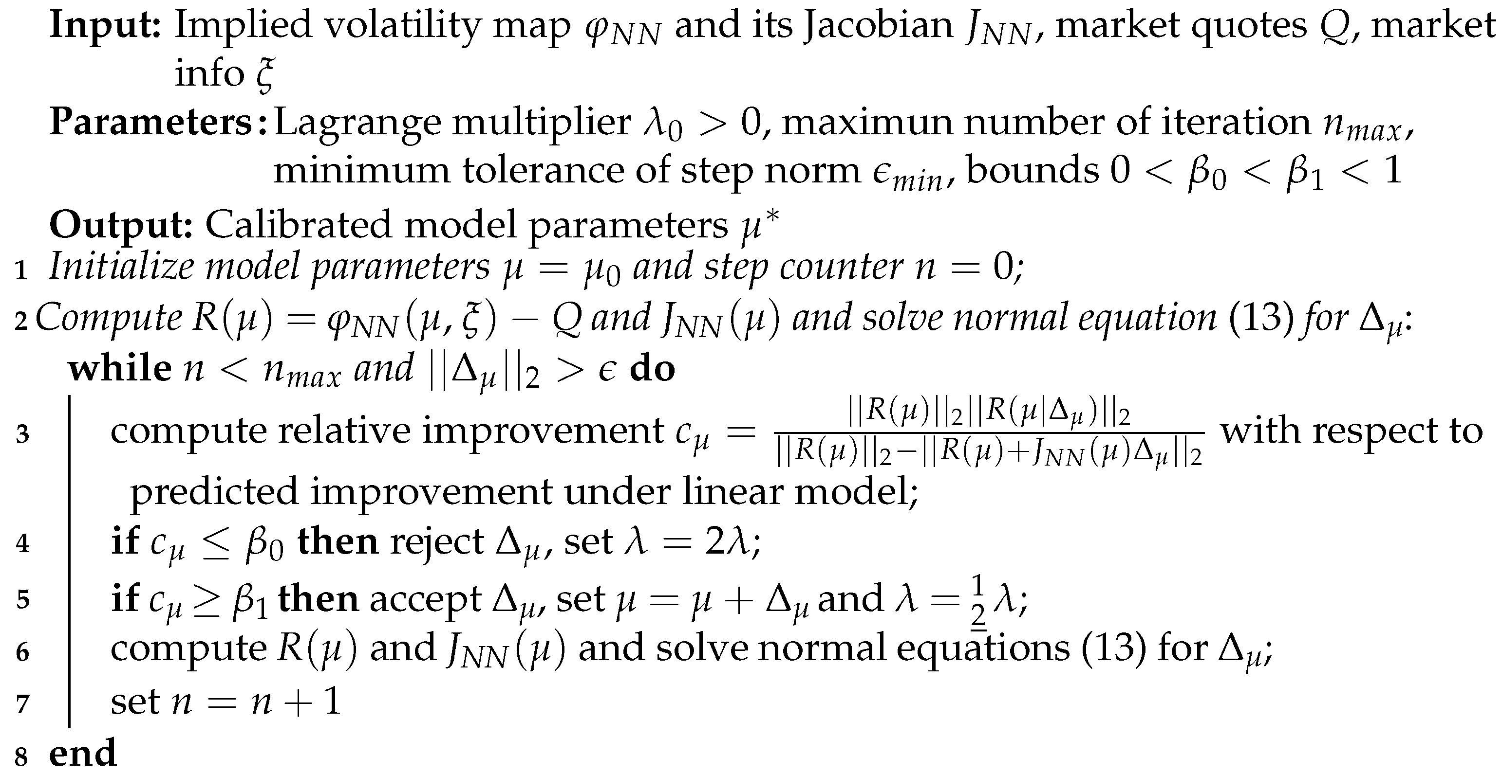
These two parameters play an important role: h m o d e l determines the capacity of S h m o d e l , while h h o p t oversees the local minimum at which the optimization procedure converges and how fast this happens. Algorithm 1 (Bayer and Stemper 2018) summarizes the main steps of the method.
Algorithm 1: Deep calibration algorithm
Risks 10 00227 i001

6. Empirical Results

In this section, we apply our findings to the solution of the Black–Scholes–Barenblatt equation as well as to calibrate the Heston model. In both cases, we start adopting the neural network structure proposed in Raissi (2018), using Tensorflow 1.1 (Abadi et al. 2016) on a HP PRO BOOK 450 G8 with an Intel Core i7-1165G7 CPU 2.80 GHz × 8 with 16 Gigabyte (GB) RAM.

6.1. Black–Scholes–Barenblatt Equation

The Black–Scholes–Barenblatt (BSB) equation (Li et al. 2019) arises from the Black–Scholes equation and generalizes it considering a nonlinear source term.
The price V ( S , t ) of an European option with underlying S is given by the famous Black–Scholes equation:
V t + 1 2 σ 2 S 2 2 V S 2 + r S V S r V = 0 .
It is important to note, that that latter equation depends on two parameters (could be functions), namely, the volatility σ and the risk-free interest rate r.
The exact choice of r and σ is not easy, but upper and lower bounds on them can be imposed with reasonable certainty. With this bounds we can compute the range and all admissible option prices.
For example, if we consider vanilla puts and calls, we know that the option prices have a monotone and convex behavior and in this case envelopes are described by a linear Black–Scholes equation. However, if we have options which prices have a different behavior (non-monotone and non-convex), then the envelopes must be found from a fully non linear equation as follow:
u t = 1 2 T r [ σ 2 d i a g ( X t 2 ) D 2 u ] + r ( u ( D u ) x ) ,
with terminal condition u ( T , x ) = g ( x ) . The latter being related to the following system of Forward–Backward SDEs:
d X t = σ d i a g ( X t ) d W t , t [ 0 , T ] X 0 = ξ d Y t = r ( Y t Z t X t ) d t + σ Z t d i a g ( X t ) d W t , t [ 0 , T ) Y T = g ( X T ) .
To verify the effectiveness and accuracy of the algorithm, we need the exact value of the solution of the BSB equation, which is given by the following lemma (Beck et al. 2019):
Lemma 1. 
Let c , σ m a x , r , T ( 0 , ) , σ m i n ( 0 , σ m a x ) , d N , let σ ¯ : R R be the function that satisfies for all x R the following:
σ ¯ ( x ) = σ m a x : x 0 σ m i n : x < 0 ,
and let g : R d R and u : [ 0 , t ] × R d R be the function that satisfies for all t [ 0 , T ] , x = ( x 1 , , x d ) R d that g ( x ) = c | | x | | R d 2 = c i = 1 d | x i | 2 and
u ( t , x ) = e x p ( [ r + | σ m a x | 2 ] ( T t ) ) g ( x ) .
Then, it holds for all t [ 0 , t ] , x = ( x 1 , , x d ) R d that u C ( [ 0 , T ] × R d , R ) , u ( T , x ) = g ( x ) , and
u t ( t , x ) + 1 2 i = 1 d | x i | 2 σ ¯ 2 u x i 2 ( t , x ) 2 2 u x i 2 ( t , x ) = r ( u ( t , x ) x , ( x u ) ( t , x ) ) R d .
Proof. 
Since u is infinitely differentiable and (21) ensures that t [ 0 , T ] , x = ( x 1 , , x d ) R d , then we have:
u ( t , x ) = e x p ( t [ r + | σ m a x | 2 ] + T [ r + | σ m a x | 2 ] ) g ( x ) .
Hence, we obtain that for all t [ 0 , T ] , x = ( x 1 , , x d ) R d , i { 1 , 2 , , d } it holds that
u t ( t , x ) = [ r + | σ m a x | 2 ] u ( t , x )
x , ( x u ) ( t , x ) ) R d = e x p ( t [ r + | σ m a x | 2 ] + T [ r + | σ m a x | 2 ] ) x , ( g ) ( x ) R d = e x p ( t [ r + | σ m a x | 2 ] + T [ r + | σ m a x | 2 ] ) x , 2 c x R d = 2 c e x p ( t [ r + | σ m a x | 2 ] + T [ r + | σ m a x | 2 ] ) | | x | | R d 2 = 2 u ( t , x )
and
2 u x i 2 ( t , x ) = 2 c e x p ( t [ r + | σ m a x | 2 ] + T [ r + | σ m a x | 2 ] ) > 0 ,
hence, exploiting (20), t [ 0 , T ] , x = ( x 1 , , x d ) R d , i { 1 , 2 , , d } , we have:
σ ¯ 2 u x i 2 ( t , x ) = σ m a x .
Equations (24)–(27) ensure that for all t [ 0 , T ] , x = ( x 1 , , x d ) R d it holds that
u t ( t , x ) + 1 2 i = 1 d | x i | 2 σ ¯ 2 u x i 2 ( t , x ) 2 2 u x i 2 ( t , x ) r ( u ( t , x ) x , ( x u ) ( t , x ) ) R d = [ r + | σ m a x | 2 ] u ( t , x ) + 1 2 i = 1 d | x i | 2 σ ¯ 2 u x i 2 ( t , x ) 2 u x i 2 ( t , x ) r ( u ( t , x ) 2 u ( t , x ) ) = [ r + | σ m a x | 2 ] u ( t , x ) + 1 2 i = 1 d | x i | 2 | σ m a x | 2 2 u x i 2 ( t , x ) + r u ( t , x ) = 1 2 i = 1 d | x i | 2 | σ m a x | 2 2 u x i 2 ( t , x ) | σ m a x | 2 u ( t , x ) = | σ m a x | 2 1 2 i = 1 d | x i | 2 2 u x i 2 ( t , x ) u ( t , x ) = | σ m a x | 2 1 2 | | x i | | R d 2 2 u x i 2 ( t , x ) u ( t , x ) = | σ m a x | 2 c | | x i | | R d 2 e x p ( t [ r + | σ m a x | 2 ] + T [ r + | σ m a x | 2 ] ) u ( t , x ) = 0 ,
so the proof is completed.   □
For simulations, we used the following parameters: T = 1 , σ = 0.4 , r = 0.05 , ξ = ( 1 , 0.5 , 1 , 0.5 , , 1 , 0.5 ) R 100 , and g ( x ) = | | x | | 2 , so that (18) becomes:
u t = 1 2 T r [ 0.16 d i a g ( X t 2 ) D 2 u ] + 0.05 ( u ( D u ) x ) u ( T , x ) = | | x | | 2 ,
and the corresponding FBSDE:
d X t = 0.4 d i a g ( X t ) d W t , t [ 0 , 1 ] X 0 = ( 1 , 0.5 , , 1 , 0.5 ) d Y t = 0.05 ( Y t Z t X t ) d t + 0.4 Z t d i a g ( X t ) d W t , t [ 0 , T ) Y 1 = | | X 1 | | 2 .
As we said before, we take the following as explicit solution of (18):
u ( t , x ) = e x p ( 0.21 ( 1 t ) ) | | x | | 2 ,
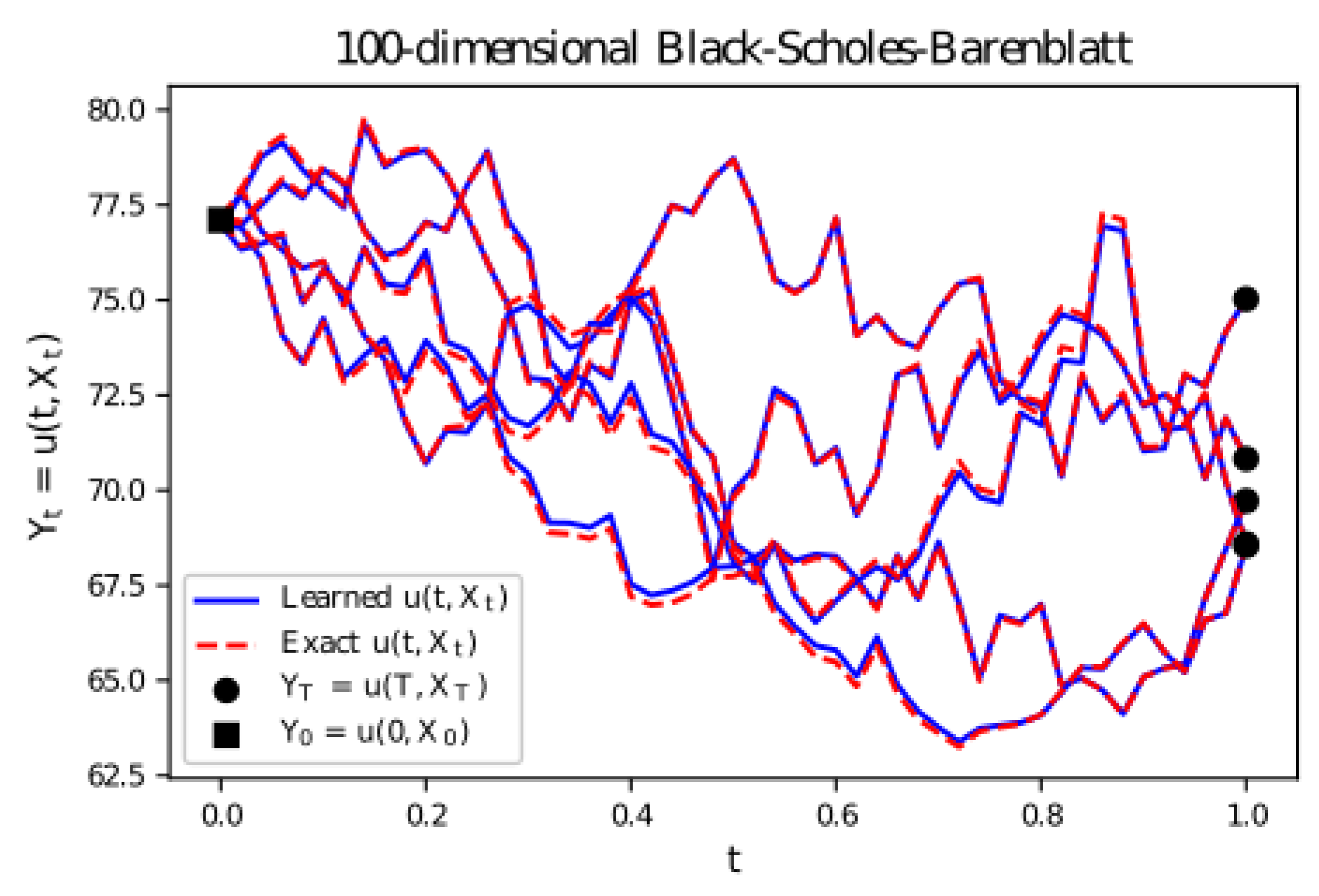
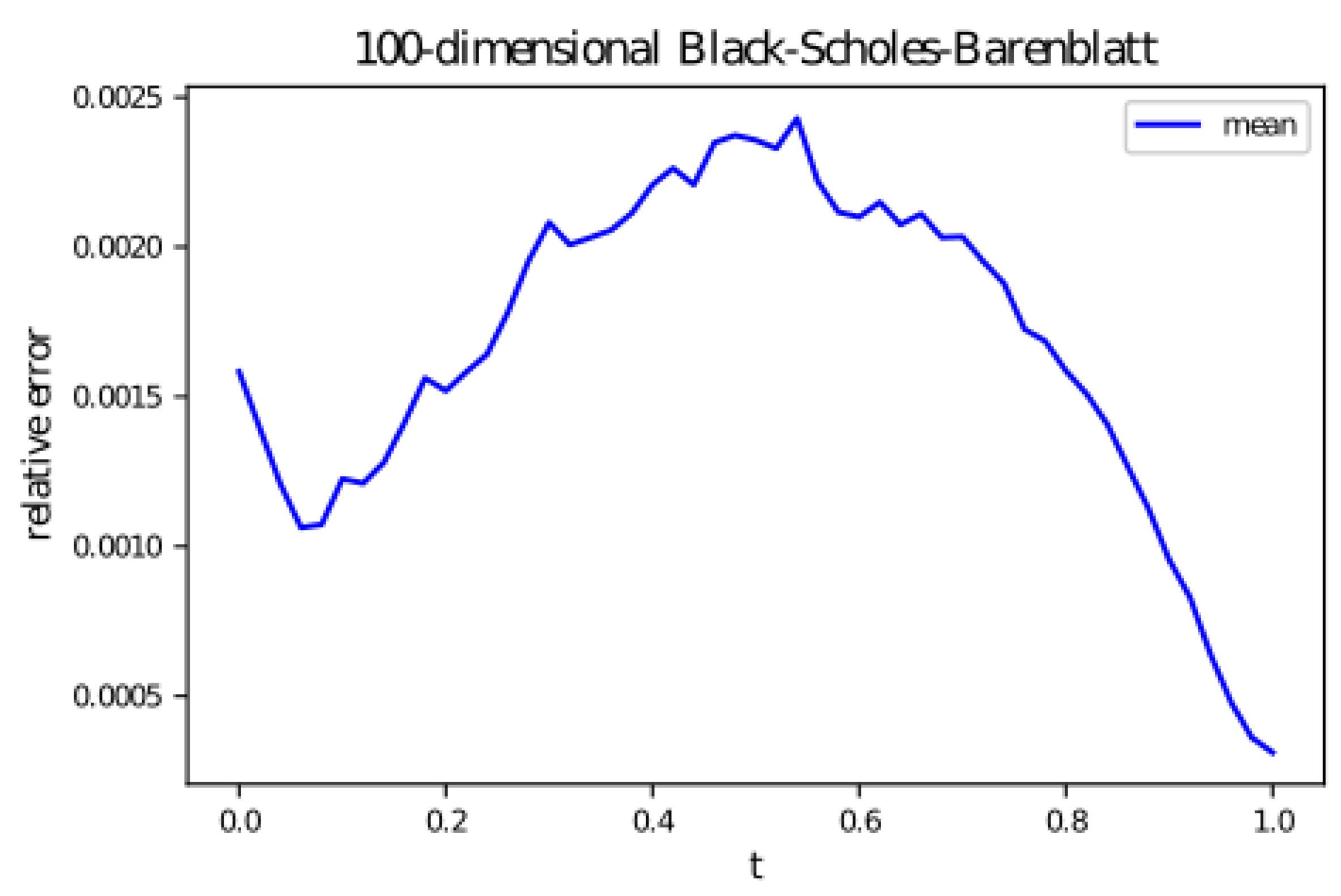
having fixed σ . We employed a 5-layer deep neural network with 256 neurons for each hidden layer to approximate the unknown solution u ( t , x ) . Time domain has been subdivided into N = 10 equally spaced interval to then apply the Adam optimizer minimizing the loss function (9) with 100 different realizations of the the underlying Brownian motion.. In Figure 2 we plot the learned solution u ( t , X t ) at a representative realizations of the underlying high-dimensional process X t . The latter shows how the whole solution, rather than only the terminal points, has been approximated. Moreover, Figure 3 shows how the error decreases in the number of Adam’s iterations, witnessing the goodness of the implemented NN-architecture in accurately approximate the exact solution u ( t , X t ) . Both pictures are obtained after, resp., 2 × 10 3 , 3 × 10 3 , 3 × 10 3 , 2 × 10 3 consecutive iterations of Adam with decreasing learning rates ( 10 3 , 10 4 , 10 4 , 10 5 ).

6.2. Heston Calibration via Neural Network

In this empirical example, we use the SPX option price data from 15 January 2018 to 9 April 2019, as in Bayer and Stemper (2018). Specifically, we focus on Time to Maturity and Strike Price to estimate the joint distribution ( M , T ) denoted with K ( M , T ) . We filter the dataset by inverse bid-ask spread, where the inverse bid-ask is the difference between the quoted prices (either by a single market maker or in a limit order book) for an immediate sale (ask) and an immediate purchase (bid) for stocks, futures contracts, options, or currency pairs in some auction scenario. The size of the bid–ask spread in a security is one measure of the liquidity of the market and of the size of the transaction cost, to consider options with a good liquidity level. In Figure 4 we can see that the higher liquidity level is concentrated in the region bounded by 0.1 m 0.29 and 1 365 T 0.2 .
For this reason, we bound the domain of IV map to this region. Now, the aim is to estimate the density distribution K ( M , T ) . We apply Kernel Density Estimate (KDE), a non-parametric way to estimate the probability density function of a random variable, using the function GrindSearchCV in scikit-learn with a Gaussian kernel to select the optimal value for the bandwidth. Then, we generate a sample of one million elements (two columns with time to maturity and moneyness) from the distribution. Finally, we add the parameters μ , ρ , λ , ν ¯ , ν 0 of Heston model extracted from a Uniform distribution U , see Table 1, and the value of IV.
Last column’s values have been computed exploiting the Heston prices function based on the Levenberg–Marquardt algorithm, see Proposition 1. The latter allows to compute European Call prices under the Heston dynamic via associated closed form solution and by using the QuantLib library (a free/open-source library for quantitative finance) providing many financially oriented solvers 1. We end up with IV values for every simulation, then used to train the neural network. In particular, we consider 900,000 samples for the training set, 45,000 for the test set and 55,000 for the validation set.
The first NN that we apply, a ReLU Fully Connected Neural Network (FCNN), is the same as the one proposed in Bayer and Stemper (2018). It is based on a 4-hidden layer NN with ReLU as activation function and 512 neurons for each layer the output layer being linear (no activation function), and with tensors denoted by rectangles.
The second NN-approach we propose belongs to the family of Recurrent Neural Network (RNN), a class of artificial NNs where connections between nodes form a directed or undirected graph along a temporal sequence. The latters, may present some problems when working with time series forecasting, as in our case. Accordingly, we choose to use a Long Short Term Memory Neural Network (LSTM) (Hochreiter and Schmidhuber 1997), which is capable of learning long-term dependencies. The chain structure is the same as RNN but, instead of a single layer, there are four layers interacting with each other in a special way.
The key ingredient of LSTMs is the cell state, the horizontal line running through the top of the diagram. The cell state is a kind of conveyor belt; it runs through the entire chain, with only a few minor linear interactions. This type of neural network has the ability to remove or add information to the cell state, carefully regulated by structures called gates. Each of this gates is composed by a sigmoid neural layer and a point-wise multiplication operation. In our case, we consider two hidden layers with 64 neurons for each one.
Once the neural networks are assembled, we train them in D t r a i n and use D v a l as a validation set. The performance are evaluated considering the loss curve generated during the training, the training time, the loss computed on the test set and the Relative Error (RE) between the IV obtained with NN and the IV computed by classic Fourier-based method:
R E ( μ , m , T ) : = | φ N N ( μ , ν 0 , e m , T ) φ ˜ ( μ , ν 0 , e m , T ) | φ ˜ ( μ , ν 0 , e m , T ) .
Both neural networks are stopped using the callback E a r l y S t o p p i n g : this allows us to decide what performance measure use in order to end training. In our case, we would seek a minimum for both validation loss and mean squared error and a maximum for validation accuracy. We impose patients (number of epoch with no improvement) equal to 3.
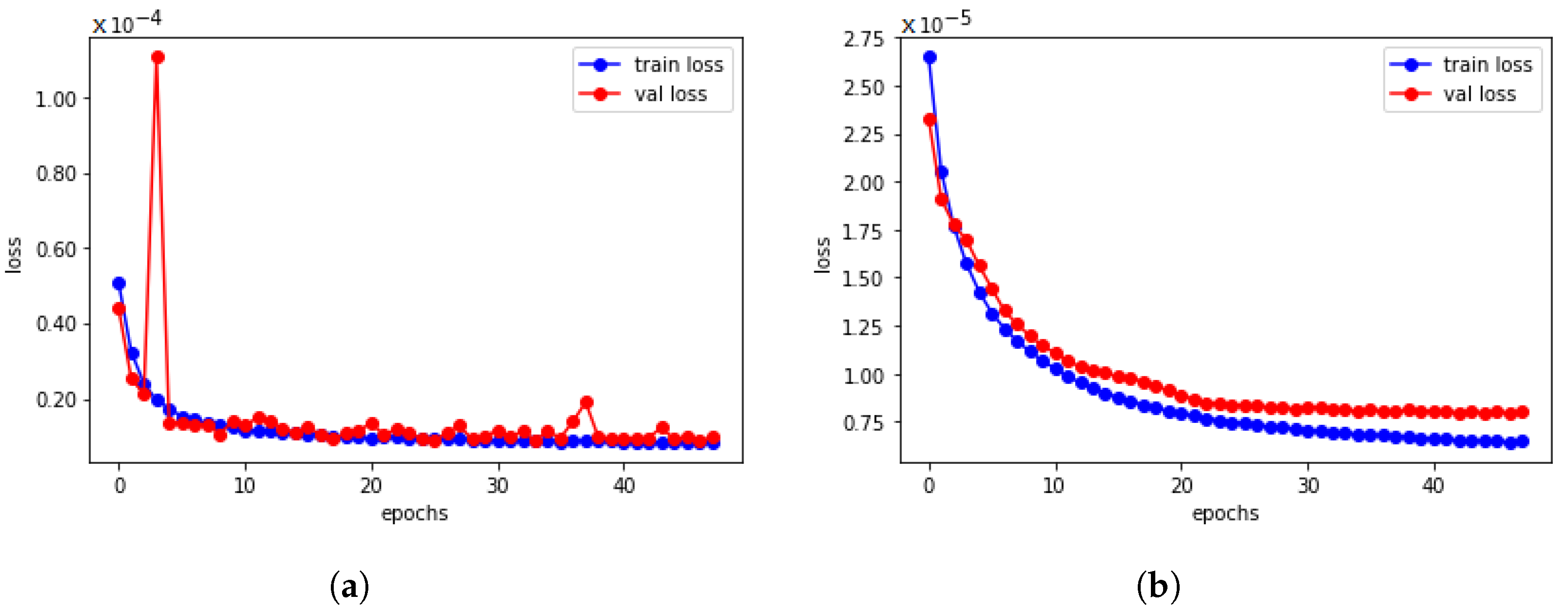
The loss curves in Figure 5 show that both neural networks have a good but different behavior. Indeed, both of them decrease quickly, but the FCNN train and the validation loss are very close to each other, with some exception epoch where the model shows a large gap between the validation and the train. This does not happen in the case of LSTM, since both curves decrease and reach a point of stability with a smaller gap.
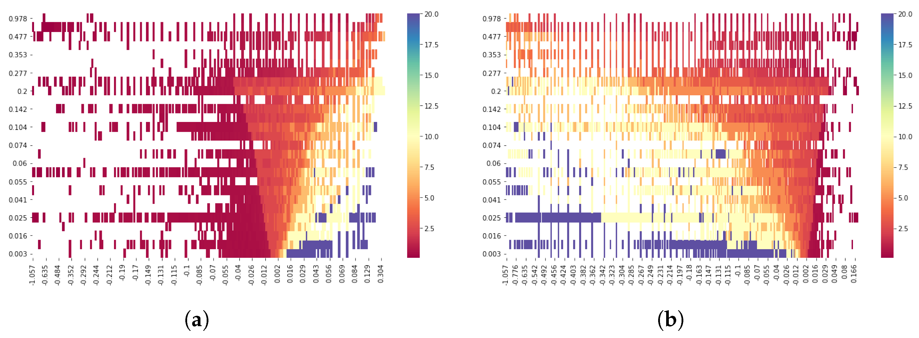
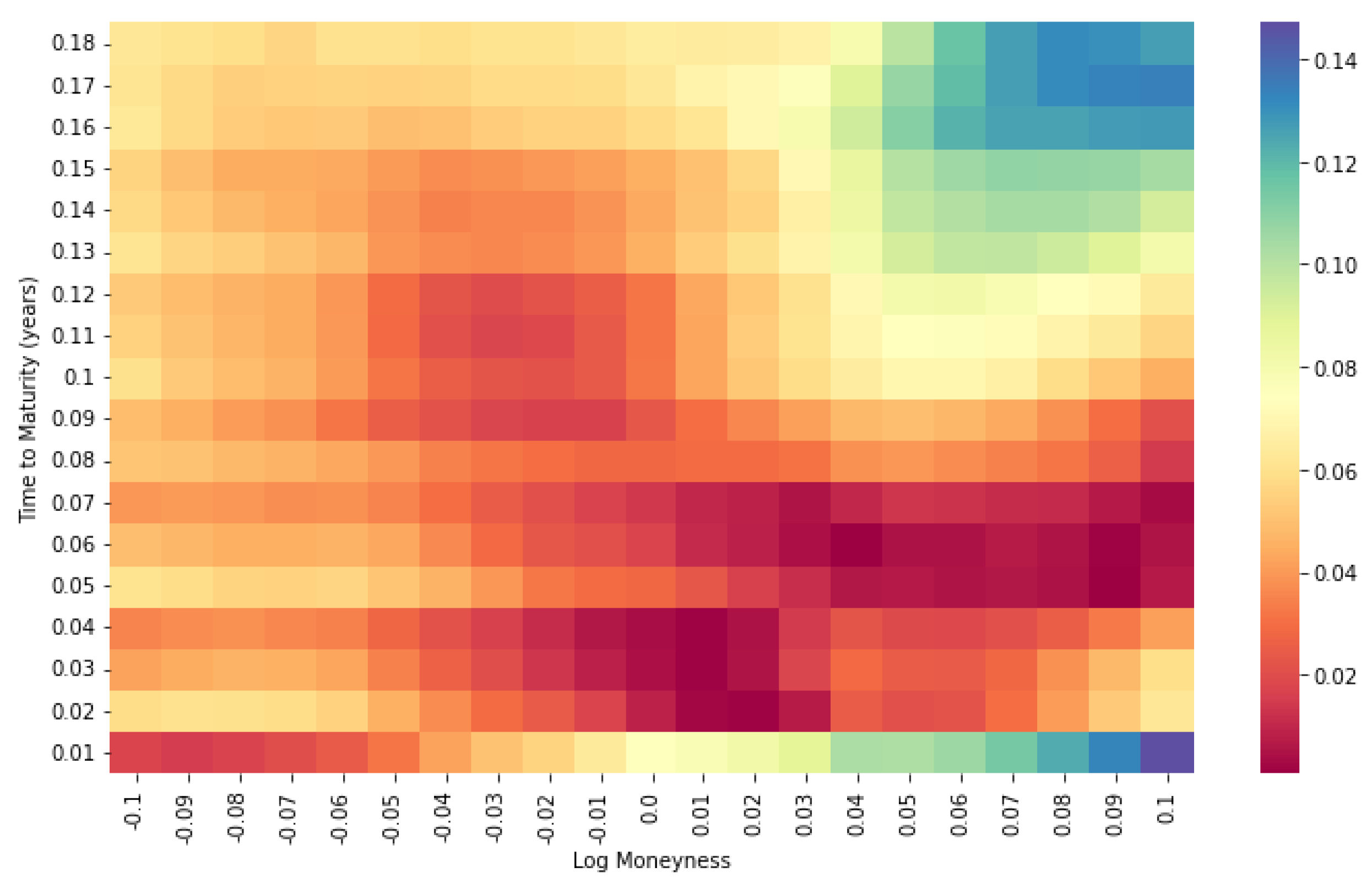
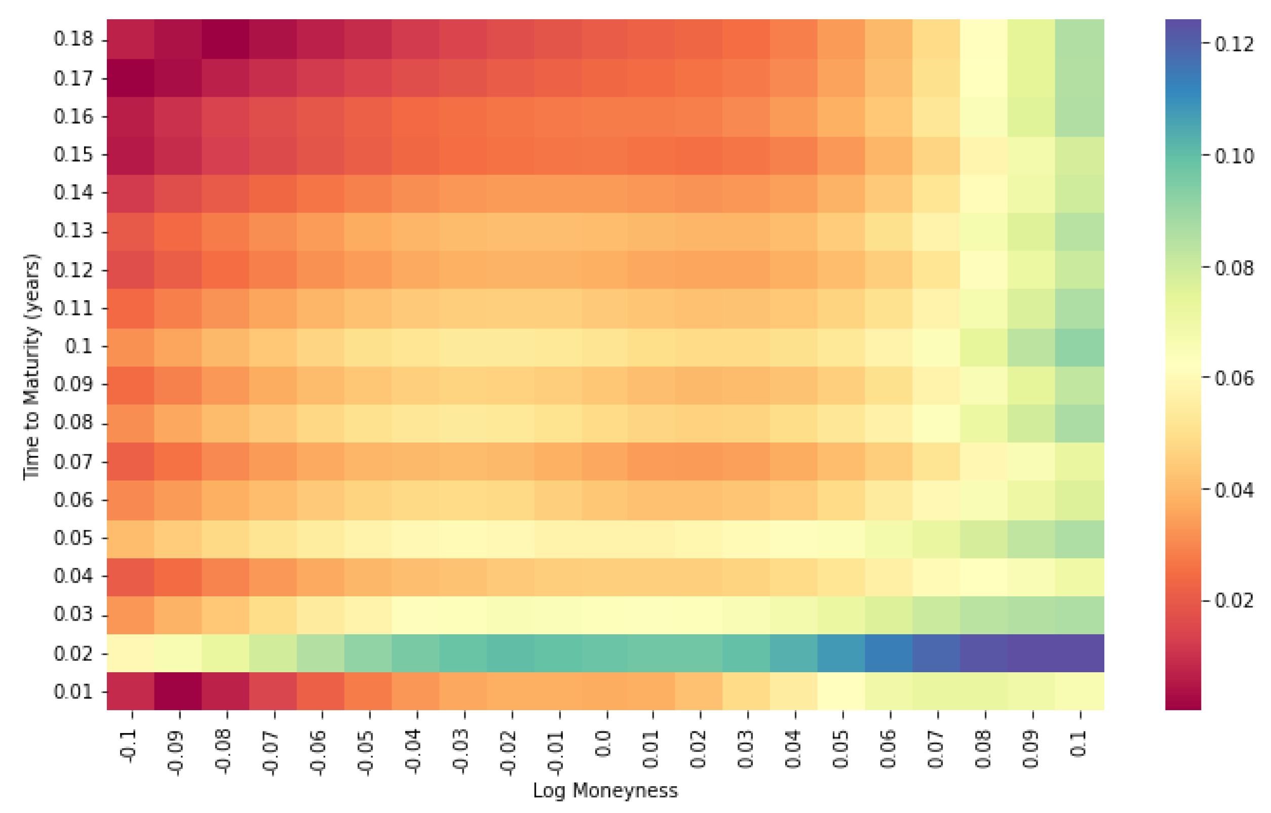
Looking at the computational time, we end up with a very import result: FCNN spend about 59 min while LSTM only 21. This huge difference suggests that LSTM might better explain the link between model parameters and the IV surface in a shorter time. This evidence is also confirmed by the errors computed on the test set and on a random dataset generated by setting the parameters of the model and varying only time to maturity and log-moneyness. The results are 9.7 × 10 6 and 3.6 × 10 6 , respectively. From Equation (29) we obtain the heatmaps with different time to maturity and log moneyness; we compute this error in a new dataset with random log moneyness and time to maturity and fixed model parameters. As the heatmap of interpolated relative errors shows, in both models there are small errors throughout most of the IV surface, with increased relative errors only for times on the short and long end, which may be attributed to less training due to less liquidity; see Figure 6 and Figure 7. The mean of DNN and LSTM are 0.09388463628 and 0.035987278, respectively.
To empirically check the goodness of the LSTM model error, we also analyzed it in a different way: we computed the difference between the value given by the NN on the test set and the true value in the dataset over the last value. The results are in Figure 8 where the normalized histogram of the relative errors in the test set is shown with quantiles. From this distribution we obtain a good approximation of φ with respect to φ N N .
Finally, the implied volatility surface generated by the two NN are shown in Figure 9.
Once the NN are trained, we are able to proceed with the calibration step. We apply the algorithm described in Algorithm 1 to initialize the parameters for the Heston model following Gatheral (2011); Table 2 reports the initialization parameters.
Using the above steps, we compute the market quotes. At this point, the deep calibration starts. First, we define a function that returns the implied volatility value and the Jacobian matrix of the NN with respect to a specific input. It will be used in the iteration step of the LM algorithm. Finally, deep calibration runs the algorithm, and after many iterations, we will get the calibrated parameters for the Heston model. A comparison between the obtained values is shown in Table 2. From the fitted values there is no clear evidence that LSTM specification outperforms the FCNN or vice-versa. Indeed, the absolute value of difference between calibrated and theoretical parameters is not better overall in neither case. However, considering the training time and the relative error in (29), we may conclude that the LSTM specification performs better.

7. Conclusions

PDEs play a fundamental role in solving many practical problems, from physics to financial mathematics. They can describe almost all time evolution models, but their solution could be problematic due to the “curse of dimensionality”. It happens because real world problems have a huge number of variables, making classic deterministic algorithms (Finite Element of Finite Difference) unfeasible. In addition, the presence of non-linear factors takes off any possibility to use probabilistic algorithms.
The growth of technology has given us powerful tools to overcome these problems. With deep learning and, in particular, with deep neural networks, we are now able to approximate the solution or part of them. In both experiments described in Raissi (2018) and Bayer and Stemper (2018), neural networks solve the course of the dimensionality problem.
The approach initially suggested by Raissi (2018) and further developed in this paper can be seen as an upgrade of the classical backward stochastic differential equation approximation provided in El Karoui et al. (1997). Furthermore, the solution of the algorithm is a function which can be evaluated not only in the initial point, but also in the whole space-time domain, see Figure 2, due to the independence between the parameters number of NN and the number of points needed to discretize the time domain. Because of its flexibility, we plan to extend the proposed NNs-based framework to consider second-order backward stochastic differential system of equations.
Concerning calibration, we have shown that the stochastic volatility model can be effectively approximated via NNs architectures, and also limited computational efforts, hence reducing execution times if compared with those related to standard numerical approaches. It is worth mentioning that, although our NN-scheme has been implemented as a regression tool, it approximates the implied volatility map with high accuracy. Moreover, to better explain the relationship between data, we showed that our LSTM-inspired solution (implemented via Keras) requires less training computation time, also with smaller loss error.
The same procedure might also be used to calibrate the optimal interest rate r. This could be conducted by using a priori on it by training the neural network on the r value.
In order to improve our performance, we also implemented a different approach, exploiting TensorFlow and building our neural network piece by piece. Nevertheless, the obtained numbers do not significantly improve that which we already obtained with our methods, despite the increased quantity of software/hardware resources needed to implement this new attempt.
Further research will be devoted to using more complex models, such as the Fractional Heston Model, to see if we are able to improve the results using more complex neural network.

Author Contributions

Formal analysis, L.D.P., E.L. and M.P.; Investigation, L.D.P., E.L. and M.P.; Methodology, L.D.P., E.L. and M.P.; Software, L.D.P., E.L. and M.P.; Writing—review & editing, L.D.P., E.L. and M.P. All authors have read and agreed to the published version of the manuscript.

Funding

This research received no external funding.

Data Availability Statement

The European option price’s time series are available at https://www.cboe.com/ (accessed on 13 September 2022).

Conflicts of Interest

The authors declare no conflict of interest.

Appendix A. Notation

W Standard Brownian motion
  
L n p ( [ 0 , T ] ) p [ 1 , ) , set of R n -valued progressively measurable
 processes Y s.t. E 0 T | Y s | p d s <
  
S 2 ( [ 0 , T ] )  space of continuous F -semimartingale Y s.t.
  E ( s u p t [ 0 , T ] | Y t | 2 ) <
  
L a d 2 ( [ 0 , T ] × Ω ; R k )  space of F -adapted process in L 2 ( [ 0 , t ] × Ω ; R k )
  
L T 2 ( R d )  space of F t -measurable random variables ξ s.t. E ( | ξ | 2 ) <
  
H T 2 ( R d )  space of predictable process Y s.t. | | Y | | 2 = E ( 0 T | Y t | 2 d t ) < )

Appendix B. Definition

Definition A1 
(Probability space). A probability space is a triple ( Ω , F , P ) where Ω is a abstract set, F is a σ algebra of subsets of the set Ω and P is a probability measure on Ω.
Definition A2 
(Random variable). A mapping X : Ω R n , n N , is called an n-dimensional random variable if, for each Borelian set B B ( B ) , we have that X 1 ( B ) F or, in other words, X is F m e a s u r a b l e .
Definition A3 
(Stochastic Process). A stochastic process is a family of random variables ξ ( t ) parameterized by t T , where T R is called parameter set.
Definition A4 
(Independent Increments). We say that a stochastic process ξ ( t ) , where t T , has independent increments if
ξ ( t 1 ) ξ ( t 0 ) , , ξ ( t n ) ξ ( t n 1 )
are independent for any t 0 < t 1 , , t n s.t. t 0 , t 1 , , t n T .
Definition A5 
(Stationary Increments). A stochastic process ξ ( t ) , where t T , is said to have stationary increments if for any s , t T with s t , the increment ξ ( t ) x ( s ) has the same probability distribution as ξ ( t s ) ξ ( 0 ) .
Definition A6 
(Martingale). A stochastic process X = { X t } { 0 is a F t -martingale w.r.t P if:
  • E P [ | X t | ] < , t 0 ;
  • E P [ X t + s | F t ] = X t , t , s 0
Definition A7 
(Adapted process). The process X is said to be adapted to the filtration F i i I if the random variable X i : Ω S is a ( F i , Σ ) -measurable function for each i I
Definition A8 
(Lèvy process). We can say that X = { X ( t ) } t 0 is a Lèvy process if:
1. 
X has independent increments, i.e., X t X s is independent of F s , 0 s < t <
2. 
X ( 0 ) = 0 a.s;
3. 
X has stationary increments, i.e., t , h X t + h X t has a distribution that is independent of t;
4. 
it is continuous in probability, i.e., t , ϵ lim s t P ( | X t X s | > ϵ ) = 0 ;
5. 
X t has cadlag trajectories, i.e., right continuous and with left limit defined everywhere.
Definition A9 
(Stopping time). A random variable τ taking values in [ 0 , T ] is called a stopping time if the event { τ t } F t t > 0 .
Definition A10 
(Pricing map). Consider a rough stochastic volatility model for an asset S with model parameters μ M R m and possibly incorporated market information ξ ε R m , then the fair price of a European Call option at time t = 0 is given by:
E [ S t ( μ , ξ M ] +
where ( M , T ) Θ R 2 are the moneyness and time to maturity. Letting:
I : = { ( μ , ξ ) × ( M , T ) | μ M , ξ ε , ( M , T ) T Θ } R m + k + 2
be the pricing input space, we then define the pricing map P 0 : I R + by:
( μ , ξ ) × ( M , T ) E [ S t ( μ , ξ M ] +
Definition A11 
(IV map). Let μ , ξ , M , T be defined as in Definition (A10). The Black and Scholes IV σ I V ( μ , ξ , M , T ) corresponding to the theoretical model price P 0 ( μ , ξ , M , T ) satisfies:
P 0 ( μ , ξ , M , T ) B S ( M , T , σ I V ( μ , ξ , M , T ) ) = ! 0 .
the function φ : I R + given by:
( μ , ξ , M , T ) σ I V ( μ , ξ , M , T ) )
is what we call the implied volatility map.

Note

1

References

  1. Abadi, Martín, Ashish Agarwal, Paul Barham, Eugene Brevdo, Zhifeng Chen, Craig Citro, Greg S. Corrado, Andy Davis, Jeffrey Dean, Matthieu Devin, and et al. 2016. Tensorflow: Large-scale machine learning on heterogeneous distributed systems. arXiv arXiv:1603.04467. [Google Scholar]
  2. Baydin, Atilim Gunes, Barak A. Pearlmutter, Alexey Andreyevich Radul, and Jeffrey Mark Siskind. 2018. Automatic differentiation in machine learning: A survey. Journal of Marchine Learning Research 18: 1–43. [Google Scholar]
  3. Bayer, Christian, and Benjamin Stemper. 2018. Deep calibration of rough stochastic volatility models. arXiv arXiv:1810.03399. [Google Scholar]
  4. Beck, Christian, Weinan E, and Arnulf Jentzen. 2019. Machine learning approximation algorithms for high-dimensional fully nonlinear partial differential equations and second-order backward stochastic differential equations. Journal of Nonlinear Science 29: 1563–619. [Google Scholar] [CrossRef] [Green Version]
  5. Bismut, Jean Michel. 1973. Conjugate convex functions in optimal stochastic control. Journal of Mathematical Analysis and Applications 44: 384–404. [Google Scholar] [CrossRef]
  6. Carleo, Giuseppe, and Matthias Troyer. 2017. Solving the quantum many-body problem with artificial neural networks. Science 355: 602–6. [Google Scholar] [CrossRef] [Green Version]
  7. Cybenko, George. 1989. Approximation by superpositions of a sigmoidal function. Mathematics of Control, Signals and Systems 2: 303–14. [Google Scholar] [CrossRef]
  8. El Karoui, Nicole, Shige Peng, and Marie Claire Quenez. 1997. Backward stochastic differential equations in finance. Mathematical Finance 7: 1–71. [Google Scholar] [CrossRef]
  9. Gatheral, Jim. 2011. The Volatility Surface: A Practitioner’s Guide. New York: John Wiley & Sons. [Google Scholar]
  10. Germain, Maximilien, Huyên Pham, and Xavier Warin. 2021. Neural networks-based algorithms for stochastic control and pdes in finance. arXiv arXiv:2101.08068. [Google Scholar]
  11. Han, Jiequn. 2016. Deep learning approximation for stochastic control problems. arXiv arXiv:1611.07422. [Google Scholar]
  12. Heston, Steven L. 1993. A closed-form solution for options with stochastic volatility with applications to bond and currency options. The Review of Financial Studies 6: 327–43. [Google Scholar] [CrossRef] [Green Version]
  13. Hochreiter, Sepp, and Jürgen Schmidhuber. 1997. Long short-term memory. Neural Computation 9: 1735–780. [Google Scholar] [CrossRef]
  14. Kingma, Diederik P., and Jimmy Ba. 2014. Adam: A method for stochastic optimization. arXiv arXiv:1412.6980. [Google Scholar]
  15. Li, Xinpeng, Yiqing Lin, and Weicheng Xu. 2019. On properties of solutions to black–scholes–barenblatt equations. Advances in Difference Equations 2019: 1–9. [Google Scholar] [CrossRef] [Green Version]
  16. Mao, Xuerong. 1995. Adapted solutions of backward stochastic differential equations with non-lipschitz coefficients. Stochastic Processes and Their Applications 58: 281–92. [Google Scholar] [CrossRef] [Green Version]
  17. Moré, Jorge J. 1978. The levenberg–Marquardt algorithm: Implementation and theory. In Numerical Analysis. Berlin: Springer, pp. 105–16. [Google Scholar]
  18. Pardoux, Etienne, and Shanjian Tang. 1999. Forward-backward stochastic differential equations and quasilinear parabolic pdes. Probability Theory and Related Fields 114: 123–50. [Google Scholar] [CrossRef]
  19. Raissi, Maziar. 2018. Forward-backward stochastic neural networks: Deep learning of high-dimensional partial differential equations. arXiv arXiv:1804.07010. [Google Scholar]
  20. Robbins, Herbert, and Sutton Monro. 1951. A Stochastic Approximation Method. The Annals of Mathematical Statistics 22: 400–7. [Google Scholar] [CrossRef]
  21. Rumelhart, David E., Geoffrey E. Hinton, and Ronald J. Williams. 1986. Learning representations by back-propagating errors. Nature 323: 533–36. [Google Scholar] [CrossRef]
  22. Sharma, Siddharth, Simone Sharma, and Anidhya Athaiya. 2020. Activation functions in neural networks. International Journal of Engineering Applied Sciences and Technology 04: 310–16. [Google Scholar] [CrossRef]
  23. Svozil, Daniel, Vladimir Kvasnicka, and Jiri Pospichal. 1997. Introduction to multi-layer feed-forward neural networks. Chemometrics and Intelligent Laboratory Systems 39: 43–62. [Google Scholar] [CrossRef]
  24. Wang, Xiaoqun. 2006. On the effects of dimension reduction techniques on some high-dimensional problems in finance. Operations Research 54: 1063–78. [Google Scholar] [CrossRef]
  25. Weinan, E, Martin Hutzenthaler, Arnulf Jentzen, and Thomas Kruse. 2019. On multilevel picard numerical approximations for high-dimensional nonlinear parabolic partial differential equations and high-dimensional nonlinear backward stochastic differential equations. Journal of Scientific Computing 79: 1534–71. [Google Scholar]
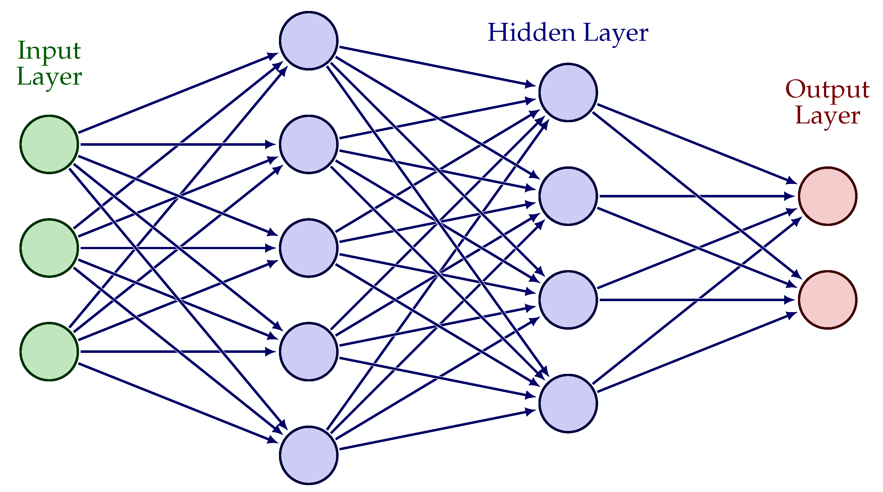
Figure 1. Example of Deep Neural Network Schema. In green the neurons of input layer, in blue the neurons of hidden layers and in red the neurons of output layer.
Risks 10 00227 g001
Figure 2. Evaluations of the learned solution Y t = u ( t , X t ) at representative realizations of the underlying high-dimensional process X t .
Risks 10 00227 g002
Figure 3. Relative error mean between exact u ( t , X t ) and approximate.
Risks 10 00227 g003
Figure 4. Liquidities by inverse bid-ask spread with traded European options. (a) Call; (b) Put.
Risks 10 00227 g004
Figure 5. Train loss and validation loss of training. (a) Loss of FCNN; (b) Loss of Multi layer LSTM.
Risks 10 00227 g005
Figure 6. Error between the theorical value and FCNN.
Risks 10 00227 g006
Figure 7. Error between the theoretic value and the LSTM.
Risks 10 00227 g007
Figure 8. Normalized histogram of RE on test set with quantiles.
Risks 10 00227 g008
Figure 9. Implied volatility surface. (a) IV FCNN; (b) IV LSTM.
Risks 10 00227 g009
Table 1. Marginal priors of the model parameters μ for synthetically generating D . The interest rate r is fixed.
ParameterMarginal
η U [ 0 , 5 ]
ρ U [ 1 , 0 ]
λ U [ 0 , 10 ]
υ ¯ U [ 0 , 1 ]
υ 0 U [ 0 , 1 ]
Table 2. Comparison between the theoretical parameters and the neural networks parameters.
ParameterTheoreticalFCNNLSTM
η 0.3877 0.3889 0.4124
ρ 0.7165 0.6871 0.7345
λ 1.3253 1.3421 1.105
ν ¯ 0.0354 0.0312 0.0401
ν 0 0.0174 0.0169 0.0171
Publisher’s Note: MDPI stays neutral with regard to jurisdictional claims in published maps and institutional affiliations.