Modeling Momentum and Reversals

Abstract

Stock prices are well known to exhibit behaviors that are difficult to model mathematically. Individual stocks are observed to exhibit short term price reversals and long term momentum, while their industries only exhibit momentum. Here we show that individual stocks can be modeled by simple mean reverting processes in such a way that these behaviors are captured, the model is arbitrage free, and market informational efficiency is preserved. Simulation shows that in such a market, when mean reversion is sufficiently high, strategies which use reversals would substantially outperform buy and hold strategies.

1. Introduction

There is a large array of literature that documents reversals and momentum in stock prices. For example, Hameed and Mian (2015) observe reversals in the best and worst subset of monthly performers within industries, whereas the industries themselves only exhibit momentum, as do stocks in the longer term. Figelman (2007) also observes long term stock momentum, albeit on a different time scale.

Many articles try to explain these behaviors by appealing to investor behavior. Daniel et al. (1998) try to explain these features via investor overconfidence and biased self-attribution. Kahneman and Tversky (1979) attribute such features to the certainty and isolation effects. Booth et al. (2016) attributes momentum and reversals to the interaction of price momentum with size related effects.

Here we develop a reduced form model for stock price movements that exhibits these behaviors. We show that reversals and momentum would be observed if stocks were mean reverting to an industry business cycle1. We analyze the model analytically and through simulation. Simulation shows that in such a market, strategies which use reversals would outperform buy and hold strategies, often by a factor of 2 or more in high mean reversion environments. We also show that this model is arbitrage free and does not violate market efficiency, thus demonstrating that reversals and momentum can exist in efficient markets.

Mean reversion as a general phenomenon is well known. Mean reversion is commonly posited for short rate models and mean reverting models are used in commodity option pricing. They are useful for modeling pairs trading, as well as analyzing the timing of entering and exiting positions Leung and Li (2015). More recently, mean reverting processes have shown up in the portfolio optimization literature Amédée-Manesme et al. (2019); Kitapbayev and Leung (2018); Zhang et al. (2020). Amédée-Manesme et al. (2019) considers mean reversion in real estate deriving from correlation to mean reverting interest rates. The other references consider assets that mean revert to a fixed constant long term mean. Our work here differs from the above literature in that the mean reversion is to a time dependent function capturing the business cycle rather than to a fixed constant. The models closest to the models we propose here show up in the commodity option pricing literature Geman (2005) and as the Black–Karasinski model in short rate modeling Brigo and Mercurio (2001), but not as equity price processes.

2. Industry and Stock Process Model

We proceed to develop what might be considered a reduced form model for stock price movements.

Consider $C_t$, the value of an industry at time t. We could model the industry value in a number of ways. If we assume the industry value is deterministic with a time dependent growth rate $g_t$, then

$$\begin{array}{c}\hfill d{C}_t=g_t{C}_{t}dt\end{array}$$

(1)

In this case, the industry value at time t is:

$$\begin{array}{c}\hfill C_t=C_0{e}^{{\int }_0^t{g}_{s}ds}\end{array}$$

(2)

If firm values follow the industry except for random perturbations away from the industry (noise), it is reasonable to assume not that the stock returns themselves are randomly perturbed, but that the firm value S itself deviates randomly from the industry, but is always equal to the industry on average. We can do that by defining

$$\begin{array}{cc}\hfill d{X}_t& =-a{X}_{t}dt+\sigma d{W}_t\hfill \end{array}$$

(3)

$$\begin{array}{cc}\hfill X_0& =0\hfill \end{array}$$

(4)

$$\begin{array}{cc}\hfill S_t& =C_t{e}^{{\alpha }_t+X_t}\hfill \end{array}$$

(5)

where W is Brownian motion, so that X is an Ornstein-Uhlenbeck process with mean reversion a and instantaneous volatility $\sigma$, and ${\alpha }_t$ is a deterministic drift chosen so that $E\left[e^{{\alpha }_t+X_t}\right]=1$. Solving the above stochastic differential equation for X yields, for times $t_1\le t_2$ that

$$\begin{array}{cc}\hfill X_{t_2}& =X_{t_1}{e}^{-a(t_2-t_1)}+e^{-a{t}_2}{\int }_{t_1}^{t_2}{e}^{at}\sigma d{W}_t\hfill \end{array}$$

(6)

Thus, X is a Gaussian process with mean and variance given by:

$$\begin{array}{cc}\hfill E\left[X_t\right]& =0\hfill \end{array}$$

(7)

$$\begin{array}{cc}\hfill \mathrm{var}\left[X_t\right]& ={\int }_0^t{e}^{-2at}{e}^{2as}{\sigma }^{2}ds\hfill \\ \hfill & =\frac{{\sigma }^2}{2a}\left(1-e^{-2at}\right)\hfill \end{array}$$

(8)

and $S_t$ is lognormal with mean

$$\begin{array}{cc}\hfill E\left[S_t\right]& =C_t{e}^{{\alpha }_t+\frac{\mathrm{var}\left[X_t\right]}{2}}.\hfill \end{array}$$

(9)

Choosing

$$\begin{array}{cc}\hfill {\alpha }_t& =-\frac{\mathrm{var}\left[X_t\right]}{2}\hfill \\ \hfill & =-\frac{{\sigma }^2}{4a}\left(1-e^{-2at}\right)\hfill \end{array}$$

(10)

then gives $S_t$ the desired mean.

Note that here we are transitioning from $C_t$ being the overall value of the industry to expressing the optimal value of a company in this industry. For simplicity, we assume all firms revert to this overall level so as to capture behavior between the industry and the economy. The relationship between the sizes of different firms could be captured by instead having each firm revert to the appropriate percentage of the total industry level, and accounting for how these percentages change over time.

Suppose a given industry has a cyclical growth rate. Say its growth rate $g_t$ is cyclical ranging from a low of l to a high of h with a period of p years, so that

$$\begin{array}{c}\hfill g_t=\frac{l+h}{2}+\frac{h-l}{2}sin(2\pi t/p).\end{array}$$

(11)

If its value strictly follows this growth rate, then its value is

$$\begin{array}{c}\hfill C_t=C_0{e}^{\frac{l+h}{2}t+\frac{(h-l)p}{4\pi }(1-cos(2\pi t/p))}.\end{array}$$

(12)

This amounts to assuming that there is an underlying deterministic hidden variable driving the value of the industry and that it has cyclic growth.

So, the model we will be considering is n stocks in a given industry, all of which are mean reverting to an overall cyclic industry level:

$$\begin{array}{cc}\hfill g_t& =\frac{l+h}{2}+\frac{h-l}{2}sin(2\pi t/p)\hfill \end{array}$$

(13)

$$\begin{array}{cc}\hfill d{C}_t& =g_t{C}_{t}dt\hfill \end{array}$$

(14)

$$\begin{array}{cc}\hfill d{X}_{i,t}& =-a_i{X}_{i,t}dt+{\sigma }_{i}d{W}_{i,t}\hfill \end{array}$$

(15)

$$\begin{array}{cc}\hfill S_{i,t}& =e^{-\frac{{\sigma }^2}{4a}\left(1-e^{-2at}\right)+X_t}\hfill \end{array}$$

(16)

where the $W_i$ are uncorrelated Brownian motions. In our simulations, we will select particular values of h and l, and use the same mean reversion and volatility for all of the stocks.

3. Model Properties

3.1. Empirical Behavior

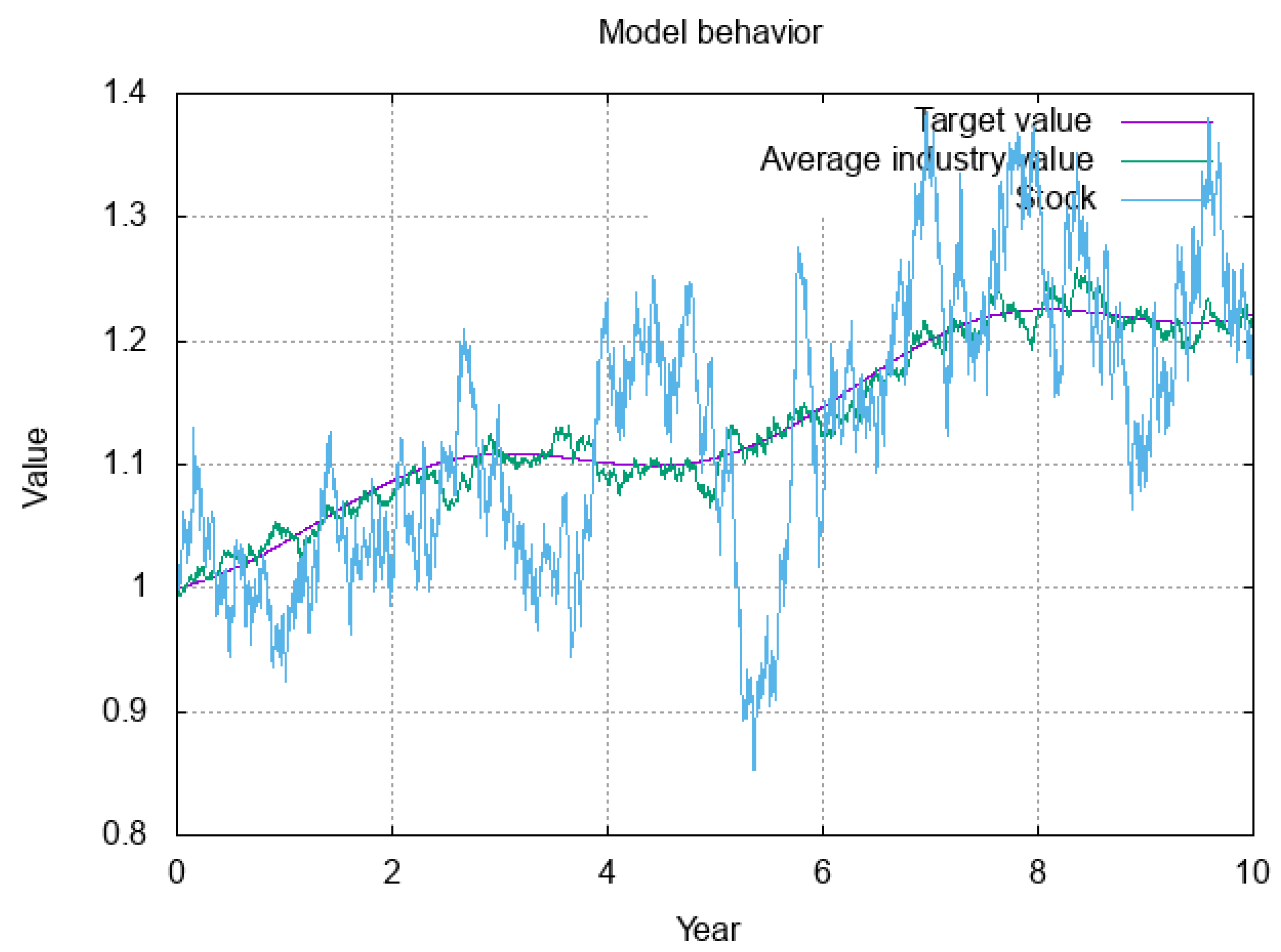
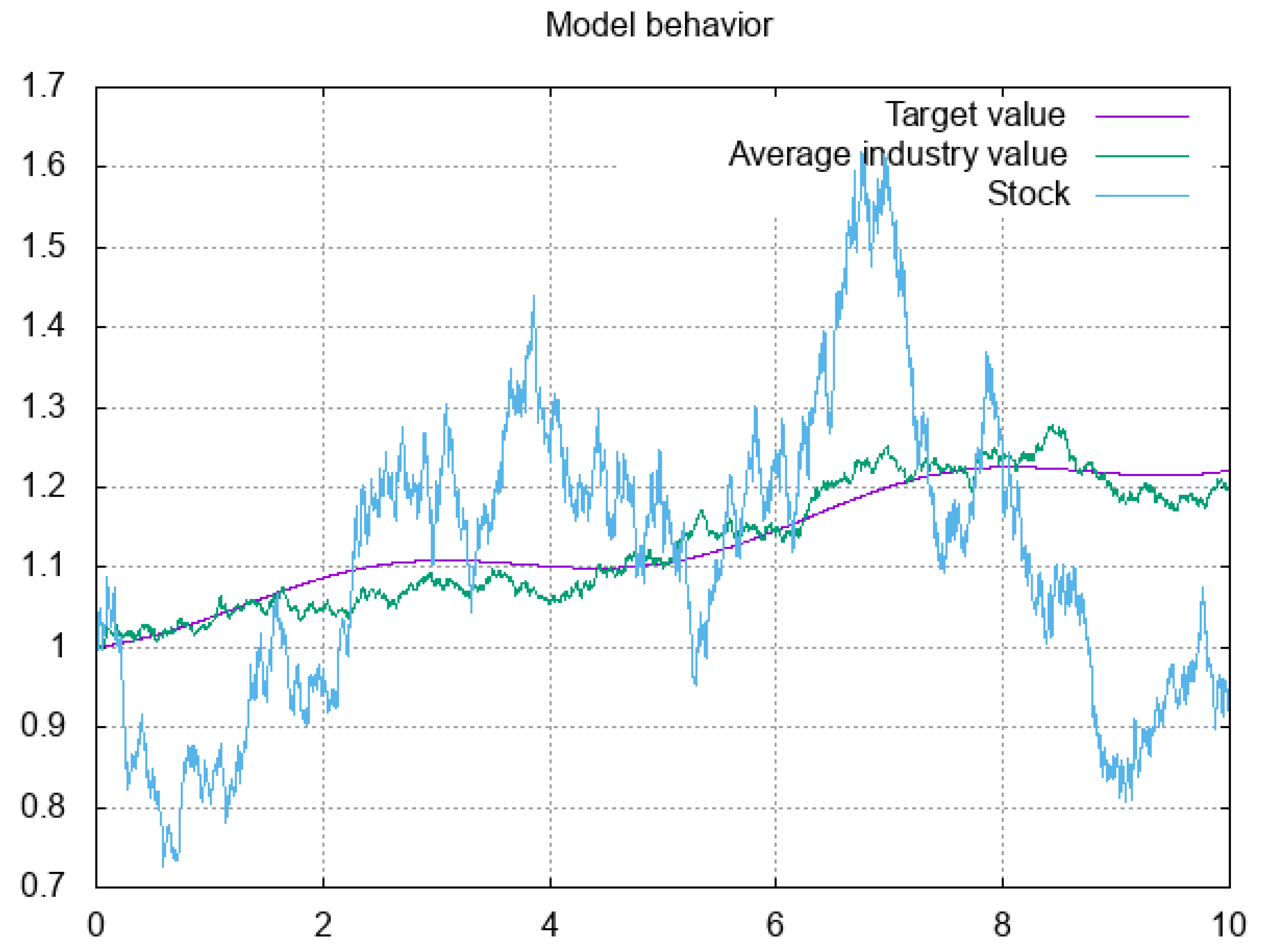
To illustrate the model behavior, we consider an industry with 30 companies. The industry follows $C_1$ with a 5 year cycle, a low rate of return of −1% and a high rate of return of 5%. Each stock has a volatility of 20%. Figure 1 and Figure 2 show the underlying dynamics with a mean reversion of 5 and of 1, respectively. We display the deterministic industry firm level, a sample path for the average stock value, and a sample path for one of the stocks in the industry. The average firm deviates around the average deterministic level, as do individual firms, albeit with much higher volatility. With lower mean reversion, the stock takes much longer to return to the industry level, and the industry does not follow the deterministic level as closely.

3.2. Bounded Variance

For a process Y following geometric Brownian motion, with

$$\begin{array}{cc}\hfill dY& =\mu Ydt+\sigma YdW\hfill \end{array}$$

(17)

for constants $\mu$ and $\sigma$, we have that

$$\begin{array}{cc}\hfill dlnY& =\left(\mu -\frac{{\sigma }^2}{2}\right)dt+\sigma d{W}_t,\hfill \end{array}$$

(18)

so the variance of $lnY$ is ${\sigma }^{2}t$, which grows without bound.

In our case,

$$\begin{array}{c}\hfill dlnS=\left(\frac{C^{\prime }}{C}+{\alpha }^{\prime }\right)dt+dX\end{array}$$

(19)

so the variance of $lnS$ equals the variance of X, which is bounded.

One might object to the model on these grounds, as this differs from the common practice of assuming stocks follow geometric Brownian motion, and thus have unbounded growth of log variance. However, there is little evidence to support such behavior of the long term variance. In practice, we can at best attempt to estimate the variance of $ln{S}_t$ from one historically observed path. For time periods greater than a year, we typically have very few samples, or overlapping (correlated) samples, or samples that span over substantial, world changing events. Not to mention the fact that changes in drift will impact sample variances. All of these issues reduce the confidence we have in assuming the variance of $ln{S}_t$ grows linearly with t, and thus of holding bounded variance as a point against this model.

3.3. Momentum and Reversals

Because the stock price process is mean reverting to $C_t$, the drift of $S_t$ is negative when $S_t>C_t$, and is positive when $S_t<C_t$. This constitutes a reversal. Since the rate of reversion is a, the reversal roughly occurs on a time scale of $1/a$. So, strong reversals on a monthly basis would constitute a mean reversion on the order of 6 to 12. Smaller mean reversions will exhibit reversals to a lesser degree.

On the other hand, the industry itself, being the sum of the values of the companies in the industry, will have greatly dampened reversal behavior. It will only exhibit reversal behavior when a large percentage of the companies have inflated values that are not compensated for by substantially deflated values of the remaining companies.

On larger time scales, since the process mean reverts to $C_t$, when the business cycle is booming, all of the industry stocks will exhibit momentum in that they are mean reverting to $C_t$ which itself exhibits momentum. Similarly, when the industry is in the bust part of the cycle, all of the industry stocks will exhibit poor long term performance.

Since reversals at the industry level are dampened, its momentum will be exhibited both on a small time scale as well as on long time scales.

3.4. Arbitrage and Market Efficiency

There has been much discussion of market efficiency since the ground breaking work of Fama (1970). Discussion has largely been about the extent to which the markets exhibit various degrees of efficiency, and the properties exhibited by efficient markets. For a general summary, see Shiller (2015).

More recently, there has been work on the relationship between market efficiency, martingale properties and the condition of a market being arbitrage free. This was first discovered by Samuelson (1965) and further elaborated on by Jensen (1978). Most recently, Jarrow and Larsson (2020) clarified and formalized the relationship between arbitrage and market efficiency. They showed that a market is informationally efficient in the sense of Fama (1970) if there exists a change of measure making the stock processes over the money market account martingales. The existence of such a change of measure also shows that the market is arbitrage free.

To see that market efficiency holds for this model, it suffices to show that there exists a change of measure making X a martingale. This suffices because it reduces us to the case where S is geometric Brownian motion with deterministic drift. The change of measure making X a martingale would have to be given by changing measure to make $W^{\prime }$ Brownian motion, where

$$\begin{array}{cc}\hfill d{W}^{\prime }& =-\frac{aX}{\sigma }dt+dW\hfill \end{array}$$

(20)

We follow the argument given by Kolmo and Eldredge (2012). By Corollary 5.14, Chapter 3 of Karatzas and Shreve (1998), it suffices to show that there exists an unbounded and increasing sequence $t_i$ with $t_0=0$ such that

$$\begin{array}{cc}\hfill E\left[e^{\frac{1}{2}{\int }_{t_i}^{t_{i+1}}\frac{a^2{X}_t^2}{{\sigma }^2}dt}\right]& <\infty \hfill \end{array}$$

(21)

for all $i\ge 0$.

Given $S\ge 0$ and $ϵ>0$, and applying Jensen’s inequality to the above exponential expression, we have that

$$\begin{array}{cc}\hfill e^{\frac{1}{2}{\int }_S^{S+ϵ}\frac{a^2{X}_t^2}{{\sigma }^2}dt}& =e^{\frac{1}{ϵ}{\int }_S^{S+ϵ}\frac{ϵa^2{X}_t^2}{2{\sigma }^2}dt}\hfill \\ \hfill & \le \frac{1}{ϵ}{\int }_S^{S+ϵ}{e}^{\frac{ϵa^2{X}_t^2}{2{\sigma }^2}}dt\hfill \end{array}$$

(22)

By Tonelli’s theorem, we can change the order of integration, so

$$\begin{array}{cc}\hfill E\left[{\int }_S^{S+ϵ}{e}^{\frac{ϵa^2{X}_t^2}{2{\sigma }^2}}dt\right]& ={\int }_S^{S+ϵ}E\left[e^{\frac{ϵa^2{X}_t^2}{2{\sigma }^2}}\right]dt.\hfill \end{array}$$

(23)

Thus, it suffices to find a constant $ϵ>0$ such that for all S, the right hand side of Equation (23) is finite. Then we can choose $t_i=iϵ$.

Since $X_t\sim N\left(0,\frac{{\sigma }^2}{2a}\left(1-e^{-2at}\right)\right)$, let ${\gamma }_t=\sqrt{\frac{{\sigma }^2}{2a}\left(1-e^{-2at}\right)}$, and $Z_t=X_t/{\gamma }_t$. Then $Z_t\sim N(0,1)$, so

$$\begin{array}{cc}\hfill E\left[e^{\frac{ϵa^2{X}_t^2}{2{\sigma }^2}}\right]& =E\left[e^{\frac{ϵa^2{\gamma }_t^2}{2{\sigma }^2}{Z}_t^2}\right]\hfill \\ \hfill & =\frac{1}{\sqrt{1-\frac{ϵa^2{\gamma }_t^2}{{\sigma }^2}}}\hfill \end{array}$$

(24)

provided that

$$\begin{array}{cc}\hfill 1-\frac{ϵa^2{\gamma }_t^2}{{\sigma }^2}& >0\hfill \end{array}$$

(25)

because $Z_t^2$ is chi-squared with one degree of freedom, so we know its moment generating function.

Solving for $ϵ$, we see that Equation 25 holds if

$$\begin{array}{cc}\hfill ϵ\left(1-e^{-2at}\right)& <\frac{2}{a}\hfill \end{array}$$

(26)

Since, for $t\ge 0$, $0\le \left(1-e^{-2at}\right)<1$, it suffices to select $ϵ=\frac{1}{a}$. Then the integrand on the right hand side of Equation 23 is continuous and bounded, and hence the integral is finite.

We conclude that the model admits an equivalent martingale measure with respect to the money market account. It then follows that the market is arbitrage free and, from Jarrow and Larsson (2020), that the model proposed here satisfies the efficient market hypothesis. We conclude that momentum and reversals can exist in efficient markets, at least in the above sense.

4. Buy Losers, Sell Winners

Due to the mean reversion, it is likely that good performance will be followed by bad performance and vise-versa. This will occur roughly on a time frame of $1/a$. If one knew the industry level $C_t$, the mean reversion a, and the volatility $\sigma$, then one could determine exactly the drift of each stock, and make an optimal decision as to which stocks to buy and which stocks to short. However, it is difficult to determine these parameters, so we will not know for sure whether the drift of $S_t$ exceeds that of the industry or lags that of the industry.

In practice, reversals are invested in based on the previous period’s returns. The strategy is to buy those with poor recent performance (buy the losers) and sell those with high recent performance (sell the winners). If reversals occur in this industry, then such a strategy should outperform the industry average. We call this the “reversals” strategy.

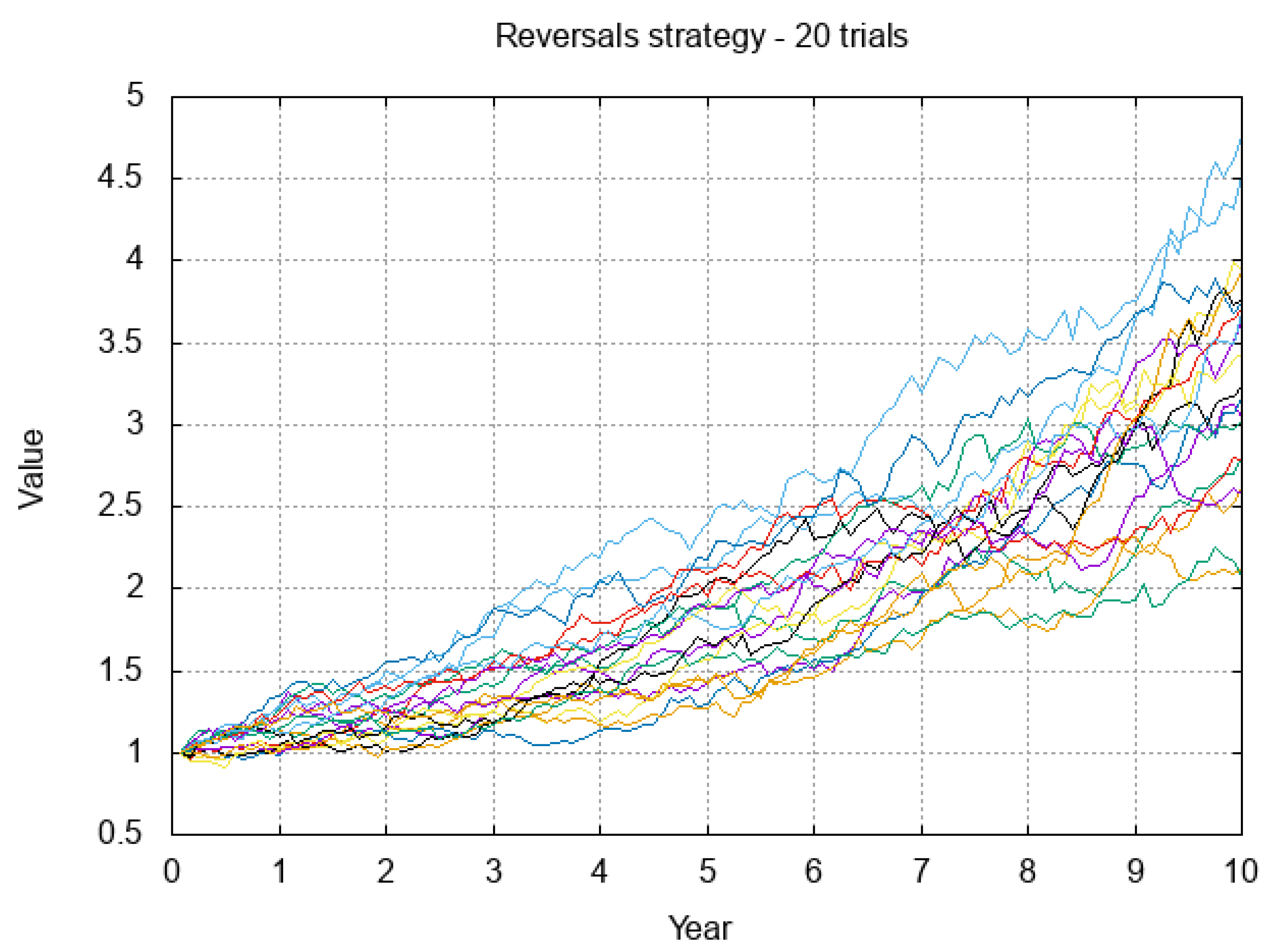
We confirm that reversals consistently occur in our model through simulation. For an industry with 30 stocks, and stock and market parameters as detailed above, we simulate the stock processes and calculate the value of the strategy which each month buys the 9 stocks (30% of the industry) whose previous month’s performance was worst, and shorts the 9 stocks with the best previous month’s performance. We repeat this experiment 20 times. Figure 3 graphs the value of the strategy over time in each of the 20 experiments over a 10 year period in the case where the mean reversion is 2. Figure 4 does the same in the case where the mean reversion is 1.

Table 1. Return statistics of the reversals strategy after 10 years for 20 industry simulations. We run the simulations for mean reversions of 1.0 and 2.0.

Statistic	MR = 1	MR = 2
mean return	6.5%	12.5%
return std	3.0%	2.5%
min return	1.1%	7.6%
25%ile return	4.1%	10.9%
50%ile return	6.8%	12.8%
75%ile return	8.4%	14.1%
max return	13.0%	16.9%

gives the mean, standard deviation and percentiles of the annualized return distribution achieved over the 20 simulations after 10 years.

With a mean reversion of 2, we observe an annualized continuous return between 7.6% and 16.9%, substantially higher than the overall industry average with the above parameters, which is about 2%. With a mean reversion of 1, the improvements are much more modest, with 4 scenarios exhibiting returns less than 4%, the largest return being 13%, and most scenario returns between 4% and 9%. One scenario returns only 1.1%, substantially below the market return of 2%. Improving on that under low mean reversion would require adjusting the strategy.

The behavior as a function of the mean reversion is given in Figure 5. Because the reversals strategy holds fewer stocks, it’s return has a higher standard deviation than holding the market. In general, the market return closely follows overall underlying return for $C_t$, which is about 2%. The performance of the reversals strategy improves on this when the mean reversion is large enough. At a mean reversion of 0.75, the average strategy return is 4.1%, double that of the market, albeit with a standard deviation of 2.8%. At a mean reversion of 1.0, the mean return is 6.5%, with a standard deviation of 3.8%. A mean reversion of 2 yields a mean return of 12% with a standard deviation of 3.1%.

5. Summary

Motivated by the observation of reversals and momentum in the stock market, we considered a stock process model where each stock in an industry reverts to an underlying deterministic cyclic level representing the industry’s business cycle. Mathematical considerations show that in such a model, one would observe short term reversals and long term momentum, while the industry would just exhibit momentum. We showed that such a model is arbitrage free, which also demonstrates that momentum and reversals can exist in efficient markets (as defined by Jarrow and Larsson (2020)).

The above analysis was tested through simulation. In simulations with the industry following a 5 year cycle with returns cycling from −1% to 5%, and stocks with volatility of 20%, we observed that once mean reversion is above about 1.0, a reversal strategy of buying the bottom 30% of the stocks (in terms of the previous month’s performance) and selling the top 30% would substantially outperform buy and hold strategies with high probability. At a mean reversion of 1, such a strategy yields a mean return of 6.5% versus a return of about 2% for the market. A mean reversion of 2 yields a mean return of 12.5% with a standard deviation of 2.5%.

References

- Amédée-Manesme, Charles-Olivier, Fabrice Barthélémy, Philippe Bertrand, and Jean-Luc Prigent. 2019. Mixed-asset portfolio allocation under mean-reverting asset returns. Annals of Operations Research 281: 65–98. [Google Scholar] [CrossRef]
- Brigo, Damiano, and Fabio Mercurio. 2001. Interest Rate Models: Theory and Practice. Berlin: Springer. [Google Scholar]
- Cerra, Valerie, Antonio Fatas, and Sweta Chaman Saxena. 2020. Hysteresis and Business Cycles. Washington, DC: International Monetary Fund. [Google Scholar]
- Daniel, Kent, David Hirshleifer, and Avanidhar Subrahmanyam. 1998. Investor psychology and security market under- and overreactions. The Journal of Finance 53: 1839–85. [Google Scholar] [CrossRef]
- Fama, Eugene F. 1970. Efficient capital markets: A review of theory and empirical work. Journal of Finance 25: 383–417. [Google Scholar] [CrossRef]
- Fernández-Villaverde, Jesús, and Pablo A. Guerrón-Quintana. 2020. Uncertainty shocks and business cycle research. Review of Economic Dynamics 37: S118–46. [Google Scholar] [CrossRef] [PubMed]
- Figelman, Ilya. 2007. Stock Return Momentum and Reversal. The Journal of Portfolio Management 34: 51–67. [Google Scholar] [CrossRef]
- Geman, Hélyette. 2005. Commodities and Commodity Derivatives: Modeling and Pricing for Agriculturals, Metals and Energy. Chichester: John Wiley & Sons. [Google Scholar]
- Geoffrey Booth, G., Hung-Gay Fung, and Wai Kin Leung. 2016. A risk-return explanation of the momentum-reversal “anomaly”. Journal of Empirical Finance 35: 68–77. [Google Scholar] [CrossRef]
- Hameed, Allaudeen, and G. Mujtaba Mian. 2015. Industries and Stock Return Reversals. Journal of Financial and Quantitative Analysis 50: 89–117. [Google Scholar] [CrossRef]
- Jarrow, Robert, and Martin Larsson. 2020. Informational efficiency with trading constraints: A characterization. SIAM Journal on Financial Mathematics 11: 959–73. [Google Scholar] [CrossRef]
- Jensen, Michael. 1978. Some anomalous evidence regarding market efficiency. Journal of Financial Economics 6: 95–101. [Google Scholar] [CrossRef]
- Kahneman, Daniel, and Amos Tversky. 1979. Prospect Theory: An Analysis of Decision under Risk. Econometrica 47: 263–92. [Google Scholar] [CrossRef]
- Karatzas, Ioannis, and Steven Shreve. 1998. Brownian Motion and Stochastic Calculus, 2nd ed. New York: Springer Science & Business Media, vol. 113. [Google Scholar]
- Kitapbayev, Yerkin, and Tim Leung. 2018. Mean Reversion Trading with Sequential Deadlines and Transaction Costs. International Journal of Theoretical and Applied Finance 21: 1850004. [Google Scholar] [CrossRef]
- Kolmo, and Nate Eldredge. 2012. Can I Apply the Girsanov Theorem to an Ornstein-Uhlenbeck Process? Available online: https://math.stackexchange.com/questions/133691/can-i-apply-the-girsanov-theorem-to-an-ornstein-uhlenbeck-process (accessed on 10 June 2022).
- Leung, Tim, and Xin Li. 2015. Optimal Mean Reversion Trading: Mathematical Analysis and Practical Applications. Singapore: World Scientific. [Google Scholar]
- Samuelson, Paul. 1965. Proof that properly anticipated prices fluctuate randomly. Industrial Management Review 6: 41–49. [Google Scholar]
- Shiller, Robert J. 2015. Irrational Exuberance. Princeton: Princeton University Press. [Google Scholar]
- Zarnowitz, Victor. 1992. Recent Work on Business Cycles in Historical Perspective. In Business Cycles: Theory, History, Indicators, and Forecasting. Chicago: National Bureau of Economic Research, University of Chicago Press, pp. 20–76. ISBN 0-226-97890-7. [Google Scholar]
- Zhang, Jize, Tim Leung, and Aleksandr Aravkin. 2020. Sparse mean-reverting portfolios via penalized likelihood optimization. Automatica 111: 108651. [Google Scholar] [CrossRef]