Financial Technical Indicator and Algorithmic Trading Strategy Based on Machine Learning and Alternative Data

Abstract

The aim of this paper is to introduce a two-step trading algorithm, named TI-SiSS. In the first step, using some technical analysis indicators and the two NLP-based metrics (namely Sentiment and Popularity) provided by FinScience and based on relevant news spread on social media, we construct a new index, named Trend Indicator. We exploit two well-known supervised machine learning methods for the newly introduced index: Extreme Gradient Boosting and Light Gradient Boosting Machine. The Trend Indicator, computed for each stock in our dataset, is able to distinguish three trend directions (upward/neutral/downward). Combining the Trend Indicator with other technical analysis indexes, we determine automated rules for buy/sell signals. We test our procedure on a dataset composed of 527 stocks belonging to American and European markets adequately discussed in the news.

1. Introduction

The automated stock picking/trading algorithms have recently gained an increasing relevance in the financial industry. The possibility of processing information from different conventional and unconventional sources gives to economic agents the opportunity to make great profits combining such information with classical financial indicators. After the advent of Big Data, new powerful computers and technologies, artificial intelligence (AI), and data science (DS) have not only increased their roles in finance but also in many different disciplines, such as cybersecurity, marketing, economics, and many others.

Frequently used algorithms for trading strategies privilege the usage of historical prices from stock markets as a tool to make decisions (buy and sell) in financial markets. Among these studies, we mention academic papers that combine supervised/unsupervised machine learning methods with information inferred directly from financial time series. For instance, Allen and Karjalainen (1999) proposed a genetic algorithm to learn technical trading rules that are strictly connected to the level of returns and volatility. More precisely, according to this work, the investor should take a long position when positive returns and low daily volatility occur and stay out of the market in the presence of negative returns and high volatility. Although Allen and Karjalainen (1999) suggested the possibility of extending their approach by including other types of information such as fundamental and macro-economic data, the main ingredients for obtaining a trading signal are the volatility and the returns. Applying the support vector machine, Lee (2009) proposed an algorithm for the identification of the direction of change in the daily NASDAQ index based on a set composed of closing prices of 20 futures contracts and nine spot indexes. Moreover, Chong et al. (2017) analyzed three unsupervised feature extraction methods (i.e., principal component analysis, autoencoder, and the restricted Boltzmann machine) to predict future market behavior using exclusively high-frequency intraday stock returns as input data. Starting from the hypothesis that financial time series contain all private/public information, Barucci et al. (2021) recently developed a trading algorithm based on financial indicators that are identified as outliers of the following series: returns, trading volume growth, bid–ask spread, volatility, and serial correlation between returns and trading volumes. These indicators have been used to identify a market signal (buy, neutral, or sell) for each security and a corresponding trading strategy (for completeness we suggest Ballings et al. 2015, for a comparison among different machine learning methods widely applied in finance for the stock price direction prediction).

However, due to the presence of different sources, a challenge for an automated trading algorithm is to take into account the investors’ opinions that some funds’ managers could underestimate by following strategies based exclusively on financial market data. For this reason, a new paradigm for constructing a trading algorithm is rising among academics and practitioners. Indeed, despite the market efficient hypothesis Fama (1970), many authors documented not only the possibility to predict future movements based on the past financial prices but also to identify a market trend using the amount of data available in unconventional sources such as social networks, blogs, thematic forum, online newspapers, and many others. These data, named hereafter Alternative Data, refer to qualitative and quantitative information and represent how a particular company (or financial instruments) is perceived by the market and how popular it is among investors. For instance, Jaquart et al. (2020) analyzed the literature on Bitcoin prediction through machine learning and identified four groups of predictors: technical (e.g., returns, volatility, volume, etc.), blockchain-based (e.g., number of bitcoin transactions), sentiment-/interest-based (e.g., bitcoin Twitter sentiment), and asset-based (e.g., returns of a connected market index) features. Among many authors, we mention, for example, Bollen et al. (2011), who investigated whether the public mood, assessed through daily Twitter posts, predicts the Bitcoin market. Starting from the observation that the increasing digitization of textual information, news, and social media have become major resources for gathering information on important financial events, Yang et al. (2017) developed a trading strategy using tweets sentiment and genetic programming optimization. Recently, Duz and Tas (2021) confirmed that firm-specific Twitter sentiment contains information for predicting stock returns and this predictive power remains significant after controlling news sentiment. Their research leads to the possibility of exploiting the social media sentiment in a trading strategy.

The aim of our work is twofold. Firstly, we contribute to the literature that studies the possibility of identifying a trend for a stock using Alternative Data and standard financial indicators. Indeed, similarly to Barucci et al. (2021), we propose a procedure based on the identification of the market trend for a specific stock. However, our classification (upward/neutral/downward) includes financial indicators and two metrics that quantify all information contained in Alternative Data. Secondly, we develop a stock picking/trading algorithm based on the results of the classification procedure.

The main instruments for our two-step trading (classification) strategy are Sentiment and Popularity metrics. These two quantities, published daily by FinScience1, are obtained by searching over 1.5 million web pages, extrapolating, interpreting, and analyzing their contents in order to identify valuable information. Sentiment, which takes values from −1 to 1, assesses the perception of the company, while Popularity, which assumes only positive values, measures investors’ interest in a topic.

The remainder of the paper is organized as follows. Section 2 reviews technical analysis market indicators used as inputs for our analysis with a discussion of the extreme gradient boosting and light gradient boosted machine used in the classification step. Section 3 introduces the Sentiment and Popularity metrics developed in FinScience; then, we discuss a supervised classification problem with the explanation of the solution for the creation of labels. Afterwards, we create a new, reliable, FinScience-metrics-based financial technical indicator that has the aim of predicting the price trend one day forward in the future. Finally, we conduct a comparison with an alternative trading strategy developed by FinScience and we also provide the gross/net performances for the most/least capitalized companies in a dataset. Section 4 concludes.

2. Technical Analysis Indicators and Machine Learning Algorithms

In this section, we describe the technical analysis indicators that will be used in the empirical part of this paper. We also briefly review the mathematical aspects of the two machine learning algorithms that we consider in our analysis: extreme gradient boosting (XGBoost) and light gradient boosted machine (LightGBM).

2.1. Technical Analysis Indicators

We classify the technical analysis indicators into two groups. The first one contains such indicators that, combined with the Sentiment and Popularity metrics, construct the Trend Indicator for each company in our dataset. By means of the XGBoost or LightGBM algorithms, the aim of the Trend Indicator is to recognize the future trend of market prices. More precisely, it returns three labels (“0”, ”1”, and “2”) where the labels “2”, “1”, and “0” denote upward, neutral, and downward trends, respectively. These technical indicators are:

1.

The Simple Moving Average (SMA), which is the sample mean of the close daily prices over a specific time interval (see Ellis and Parbery 2005, for more details). Therefore, to assess the short-, medium-, and long-term price directions, we include in our analysis SMA for 7, 80, and 160 days, respectively.

2.

The Average True Range (ATR) measures the price variation over a specified time interval. We refer to Achelis (2001) for its formal definition. In the empirical analysis, we focus on the effect of the variability in a short time interval, i.e., 7 days.

3.

The Relative Strength Index (RSI) measures the magnitude of the price changes Levy (1967). This indicator ranges from 0 to 100, with two thresholds indicating the oversold at level 30 and overbought at level 70. In our analysis, we include this index with a 7-day time-horizon.

4.

The Donchian Channel (DC) is used to detect strong price movements, looking for either a candlestick breaking the upper ceiling (for bullish movements) or the lower floor (for bearish ones).

All the aforementioned indicators were used as inputs in the machine learning supervised models, except the DC indicator, whose variations represent the output of the models. If the DC predicted variation is positive, then Trend Indicator assumes label “2”, label “0” if DC variation is negative, and label “1” if DC’s line is flat. For DC, we consider a 5-day time horizon.

The second family contains the indicators that, combined with the Trend Indicator, will be used in a signal buying/selling strategy. More precisely, they are used as inputs in our stock picking/trading algorithm. In this second group, we include the SMA indicator and the technical analysis indicators reported below:

1.

The Average Directional Index (ADI) measures the trend’s strength but without telling us whether the movement is up or down. The ADI ranges from 0 to 100, and a value above 25 points out the fact that the trend of the price company is strong enough for being traded.

2.

The Momentum Indicator (MOM) is an anticipatory indicator that measures the rate of the rise or fall of stock prices (see Thomsett 2019, and references therein).

In the empirical analysis, we use these indexes with a 7-day time-horizon. Our classification is motivated by the fact that SMA, ATR, RSI, and DC are widely used for capturing the price movements while the remaining indicators are able to capture the buying/selling time. In fact, the ADI indicates the existence of a trend movement while MOM tells us the direction of such movement; therefore, a change of MOM sign could be translated in a buying/selling signal.

2.2. Extreme Gradient Boosting and Light Gradient Boosted Machine Algorithms

In this section we present the basic theory behind the selected models: the XGBoost and the LightGBM algoritms. Both numerical procedures come from the same macro-family of decision-tree-based procedures, but they are the most complicated and performant models since they represent the most advanced level of boosting.

The XGBoost algorithm, developed by Chen and Guestrin (2016), is characterized by the following steps:

• It computes second-order gradients to understand the direction of gradients themselves.
• It uses ${\mathrm{L}}^1$, ${\mathrm{L}}^2$ regularizations and tree pruning to prevent overfitting.
• It parallelizes on your own machine for improving the velocity of the computations.

Letting $x_1,\dots ,x_n$ be the vector inputs containing n features and $y_1,\dots ,y_n$ the corresponding observed outputs, a tree ensemble model combines K trees to obtain the estimated outputs, that is:

$$\widehat{y_i}=\sum _{k=1}^K{f}_k\left(x_i\right)$$

1.

where each $f_k$ is a prediction from the k-th decision tree. With this model construction, the train phase is carried out by minimizing a regularized loss function between the observed and predicted outputs. For a multiclassification problem, that is our case, the multiclass logistic loss function (mlogloss) can be used. Let the true labels for a set of samples be encoded as a 1-of-J binary indicator matrix Y, i.e., $y_{i,j}$ = 1 if sample i has label j taken from a set of J labels. Let P be a matrix of probability estimates, with $p_{i,j}=\mathrm{Pr}(y_{i,j}=1)$. Then, the mlogloss L is defined as:

$$L=-{\displaystyle \frac{1}{N}}\sum _{i=1}^N\sum _{j=1}^M{y}_{i,j}log\left(p_{i,j}\right).$$

2.

Moreover, another important aspect is the regularization phase, in which the model controls its complexity, preventing the overfitting problem. The XGBoost algorithm uses the following regularizing function:

$$\mathsf{\Omega }=\gamma T+{\displaystyle \frac{1}{2}}\lambda \sum _{j=1}^T{{\omega }_j}^2$$

(3)

where T is the number of leaves on a tree, ${\omega }_j\in {\mathbb{R}}^T$ is the score on the j-th leaf of that tree, $\gamma$ and $\lambda$ are, instead, the parameters used for controlling the overfitting, respectively, setting the minimum gain split threshold and degree of regularization for ${\mathrm{L}}^1$ or ${\mathrm{L}}^2$. Combining (2) and (3), we have the objective function used in the minimization problem:

$$\mathrm{Obj}=\sum _{i}l(\widehat{y_i},y_i)+\sum _k\mathsf{\Omega }\left(f_k\right)$$

(4)

where the first sum is used for controlling the predictive power; indeed, $l\left(\widehat{y_i},y_i\right)$ is a differentiable convex loss function that measures the difference between the prediction $\widehat{y_i}$ and the target $y_i$, while the remaining term in (4) is used for controlling the complexity of the model itself. The XGBoost procedure exploits the gradient descent algorithm to minimize the quantity in (4): it is an iterative technique that computes the following equation at each iteration (given an objective function).

$${\displaystyle \frac{\partial \mathrm{Obj}(y,\widehat{y})}{\partial \widehat{y}}}$$

Then, the prediction $\widehat{y}$ is improved along with the direction of the gradient, to minimize the objective (actually, in order to make XGBoost convert faster, it also takes into consideration the second-order gradient using the Taylor approximation since not all the objective functions have derivatives). Therefore, in the end, removing all the constant terms, the resulting objective function is   

$${\mathrm{Obj}}^{\left(t\right)}=\sum _{i=1}^n[g_i{f}_t\left(x_i\right)+{\displaystyle \frac{1}{2}}{h}_i{f}_t^2\left(x_i\right)]+\mathsf{\Omega }\left(f_t\right)$$

(5)

where $g_i={\displaystyle \frac{\partial l(y_i,{\widehat{y}}^{(t-1)})}{\partial {\widehat{y}}^{(t-1)}}}$ and $h_i={\displaystyle \frac{{\partial }^{2}l(y_i,{\widehat{y}}^{(t-1)})}{\partial {\widehat{y}}^{(t-1)}}}$.

Therefore, (5) is the objective function at the t-th step and the goal of the model is to find an $f_t$ that optimizes this quantity.

The main problem is to obtain a tree that improves predictions along with the gradient. To find such a tree it is necessary to answer to two further questions:

1.

How can we find a good tree structure?

2.

How can we assign prediction scores?

First, let us assume we already have the answer to the first question and let us try to answer the second question. It is possible to define a tree as

$$f_t\left(x\right)={\omega }_{q\left(x\right)}$$

(6)

where ($q:{\mathbb{R}}^m\to T$) is a “directing” function which assigns every data point to the $q\left(x\right)$-th leaf, such as $F=\{f\left(X\right)={\omega }_q\left(x\right)\}$. Therefore, it is possible to describe the prediction process as follows:

• Assign the data point x to a leaf by q.
• Assign the corresponding score ${\omega }_{q\left(x\right)}$ on the $q\left(x\right)$-th leaf to the data point.

Then, it is necessary to define the set that contains the indices of the data points that are assigned to the j-th leaf as follows:

$$I_j=\left\{i\right|q\left(x_i\right)=j\}$$

Thus, now it is possible to rewrite the objective function as

$$\begin{array}{ccc}\hfill {\mathrm{Obj}}^{\left(t\right)}& =& \sum _{i=1}^n[g_i{f}_t\left(x_i\right)+{\displaystyle \frac{1}{2}}{h}_i{f}_t^2\left(x_i\right)]+\gamma T+{\displaystyle \frac{1}{2}}\lambda \sum _{j=1}^t{\omega }_j^2\hfill \\ & =& \sum _{j=1}^T[(\sum _{i\in I_j}^{}{g}_i){\omega }_j+{\displaystyle \frac{1}{2}}(\sum _{i\in I_j}^{}{h}_i+\lambda ){\omega }_j^2]+\gamma T\hfill \end{array}$$

(7)

In (7), the first part has a summation over the data points, but in the second one the summation is performed leaf by leaf for all the T leaves. Since it is a quadratic problem of ${\omega }_j$, for a fixed structure $q_{\left(x\right)}$, the optimal value is

$${\omega }_j^{*}={\displaystyle \frac{{\sum }_{i\in I_j}^{}{g}_i}{{\sum }_{i\in I_j}^{}{h}_i+\lambda }}$$

and, therefore, simply substituting, the corresponding value of the objective function is

$${\mathrm{Obj}}^{\left(t\right)}=-{\displaystyle \frac{1}{2}}\sum _{j=1}^T{\displaystyle \frac{{\left({\sum }_{i\in I_j}^{}{g}_i\right)}^2}{{\sum }_{i\in I_j}^{}{h}_i+\lambda }}+\gamma T$$

(8)

where the leaf score ${\omega }_j$ is always related to the first and second order of the loss function g and h and the regularization parameter $\lambda$. This is how it is possible to find the score associated with a leaf assuming to know the structure of a tree.

Now, we move back to the first question: how can we find a good tree structure? Since this is a difficult question to answer, a good strategy is to split it into two sub-questions:

1.

How do we choose the feature split?

2.

When do we stop the split?

Starting from question number one, the first thing to say is that in any split the goal is, of course, to find the best split-point that will optimize the objective function; therefore, for each feature it is crucial to first sort the numbers, then scan the best split-point and finally choose the best feature.

Every time that a split is performed, a leaf is transformed into an internal node having leaves with different scores than the initial one.

Clearly, the principal aim is to calculate the gain (or the eventual loss) obtained from such a split. Usually, in other tree-based algorithms, the computation of this gain is generally made through the Gini index or entropy metric, but in the XGBoost this calculation is based on the objective function. In particular, XGBoost exploits the set of indices I of data points assigned to the node, where $I_L$ and $I_R$ are the subsets of indices of data points assigned to the two new leaves. Now, recalling that the best value of the objective function on the j-th leaf is (8) without the first summation and the T value in the last term, the gain of the split is:

$$\mathit{gain}={\displaystyle \frac{1}{2}}\left[{\displaystyle \frac{{\left({\sum }_{i\in I_L}{g}_i\right)}^2}{{\sum }_{i\in I_L}^{}{h}_i+\lambda }}+{\displaystyle \frac{{\left({\sum }_{i\in I_R}{g}_i\right)}^2}{{\sum }_{i\in I_R}^{}{h}_i+\lambda }}-{\displaystyle \frac{{\left({\sum }_{i\in I}{g}_i\right)}^2}{{\sum }_{i\in I}^{}{h}_i+\lambda }}\right]-\gamma$$

where:

• ${\displaystyle \frac{{\left({\sum }_{i\in I_L}{g}_i\right)}^2}{{\sum }_{i\in I_L}^{}{h}_i+\lambda }}$    is the value of the left leaf;
• ${\displaystyle \frac{{\left({\sum }_{i\in I_R}{g}_i\right)}^2}{{\sum }_{i\in I_R}^{}{h}_i+\lambda }}$    is the value of the right leaf;
• ${\displaystyle \frac{{\left({\sum }_{i\in I}{g}_i\right)}^2}{{\sum }_{i\in I}^{}{h}_i+\lambda }}$    is the objective of the previous leaf;
• $\gamma$ is the parameter which controls the number of leaves (i.e., the complexity of the algorithm).

To understand whether when transforming one leaf into two new leaves there is an improvement of the objective or not, it is enough to look at the value (positive or negative) of this gain. Therefore, in conclusion, the XGBoost algorithm, to build a tree, first finds the best split-point recursively until the maximum depth (specifiable by the user) is reached and then it prunes out the nodes with negative gains with a bottom-up order.

LightGBM is a fast, distributed, high-performance tree-based gradient boosting framework developed in Ke et al. (2017). The most important features of this algorithm that differentiate it from XGBoost are the faster training speed and the fact that it supports parallel, distributed, and GPU learning and that it is capable of handling large-scale data. Another main difference between LightGBM and XGBoost is the way in which they grow a tree: the first one uses leaf-wise tree growth, expanding those leaves that bring a real benefit to the model, while the second uses level-wise tree growth, expanding the tree one level at a time and then cutting off the unnecessary branches at the end of the process.

The first thing that makes LightGBM faster in the training phase is the way it sorts the numbers: this algorithm takes the inputs and divides them into bins, reducing a lot of the computation effort needed to test all the possible combinations of splits. This process, called histogram or bin way of splitting, clearly makes computations much faster than the ones of XGBoost. The second improving characteristic of this algorithm is called exclusive feature bundling (EFB), which reduces the dimension of the features that are mutually exclusive. For example, if there are two features, green and red, which correspond to the color of a financial candle, taking either value 1 or 0 based on the corresponding candlestick’s color, then these features are mutually exclusive since a candle cannot be green and red at the same time. Thus, this process creates a new bundled feature with a lower dimension, using new values for identifying the two cases, which in this situation are number 11 for the green candle and number 10 for the red one. Therefore, by reducing the dimensionality of some of the input features, the algorithm is able to run faster, since it has fewer features to evaluate. The third characteristic that differentiates LightLGBM from XGBoost is the so-called gradient-based one side sampling (GOSS), which helps the LightLGBM algorithm to iteratively choose the sample to use for the computations. Suppose that the dataset used has 100 features, then the algorithm computes 100 gradients $G_1,G_2,\dots ,G_{100}$ and sorts them in descending order, for example, $G_{73},G_{24},\dots ,G_8$. Then, the first 20% of these records are taken out and an additional 10% is also randomly taken from the remaining 80% of gradient records. Therefore, since the gradients are descendingly ordered, the algorithm takes only the 10% of the features on which it performs well and the 20% of those features on which it performs poorly (high gradient means high error), thus, on which it still has a lot to learn. Afterwards, these two percentages of features are combined together, creating the sample on which the LGBM trains, calculates the gradients again, and again applies the GOSS in an iterative way.

3. Materials and Methods

In this section, we present our two-step trading algorithm. First of all, we describe the main features of the dataset. We discuss the construction and the characteristics of Popularity and Sentiment metrics that have been published daily since 2019 for each company in the dataset. Using these two metrics, we show the Python implementation for the construction of the Trend Indicator and we report some results about its ability in market phase prediction. Further, we present our strategy, named Techincal Indicator—Signal Screener Strategy (TI-SiSS), for the identification of buying/selling signals. A component of TI-SiSS is the Trend Indicator that, combined with SMA, gives us trend-increasing stocks suitable for our strategy (filtering phase). For completeness, the timing phase is composed of Popularity variation and Sentiment level and provides us with buying/selling time instants. Then, we compare TI-SiSS with a similar strategy that does not include the Trend Indicator. Finally, we analyze gross and net performances of TI-SiSS for the five most/least capitalized companies in the dataset. Figure 1 shows a flow diagram that describes our new two-step algorithm.

3.1. Dataset

In our analysis, we consider a dataset containing the daily market closing prices for 527 companies. The period of observation ranges from 25 September 2019 to 18 February 20222. Figure 2 shows the distribution of companies for industrial sectors and geographical areas. The most represented sector is the Information Technology, with 117 companies while the USA companies are 91% of the dataset.

Table 1. Main information about the top 5 most/least capitalized stocks in the dataset. MDD stands for maximum drawdown.

Stock	Mrk. Cap. (bn)	Max/Min Pop.	Max/Min Sent.	Mean	S.D.	Skew.	Kurt.	MDD
Apple	2260	$1.91\times {10}^7$/$9.87\times {10}^6$	0.32/−0.25	$1.98\times {10}^{-3}$	0.022	−0.246	6.000	−70.5%
Microsoft	1710	$9.87\times {10}^6$/$3.45\times {10}^5$	0.30/−0.21	$1.25\times {10}^{-3}$	0.021	−0.465	10.662	−61.6%
UnitedHealth	467	$4.99\times {10}^5$/8.650	0.64/−0.64	$5.18\times {10}^{-4}$	0.021	−0.653	15.298	−62.4 %
J&J	422	$8.19\times {10}^5$/196	0.52/−0.49	$5.18\times {10}^{-4}$	0.014	−0.017	8.343	−40.0%
Exxon	412	$9.94\times {10}^5$/432	0.49/−0.59	$4.25\times {10}^{-4}$	0.025	−0.098	4.286	−66.2%
Tejon Ranch	3.844	9304/0	0.72/−0.69	$-4.5\times {10}^{-6}$	0.027	0.529	6.924	−37.1%
Entravision	3.482	1808/0	0.85/−0.66	$1.6\times {10}^{-3}$	0.044	$-2.8\times {10}^{-3}$	2.974	−87.6%
Community Health	2.802	$1.48\times {10}^4$/0	0.76/−0.66	$2.6\times {10}^{-3}$	0.057	0.469	4.039	−85.5%
Provident Financial	1.035	$1.05\times {10}^4$/0	0.96/−0.66	$-2.5\times {10}^{-4}$	0.029	−0.364	10.233	−48.2%
Jones Soda	0.286	3244/0	0.67/−0.64	$8.9\times {10}^{-4}$	0.070	0.584	6.887	−90.9%

reports the main statistics for the five most/least market capitalized stocks and we observe that the daily log-returns show generally a negative skewness with a high kurtosis, denoting a departure from the normality assumption.

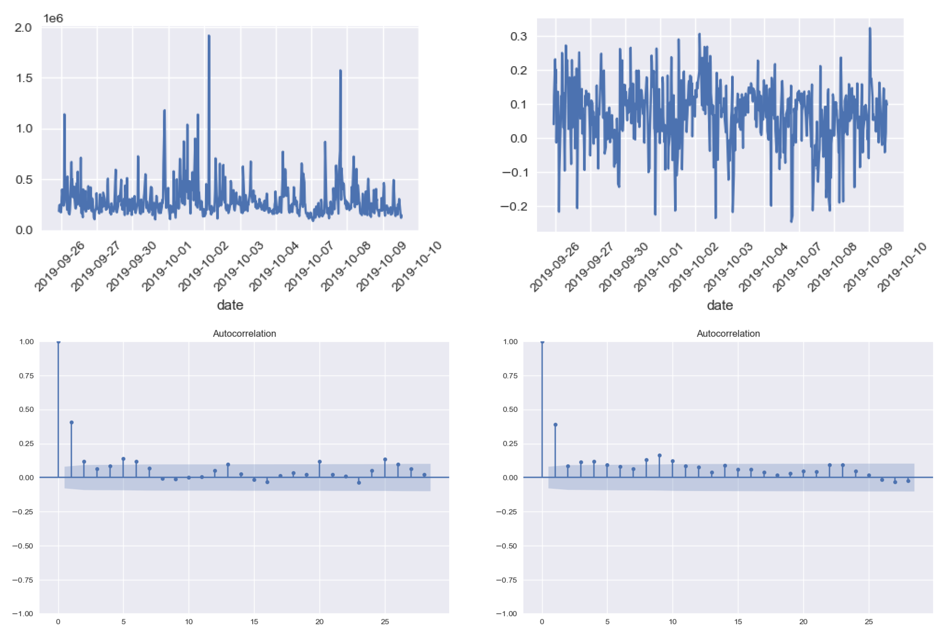
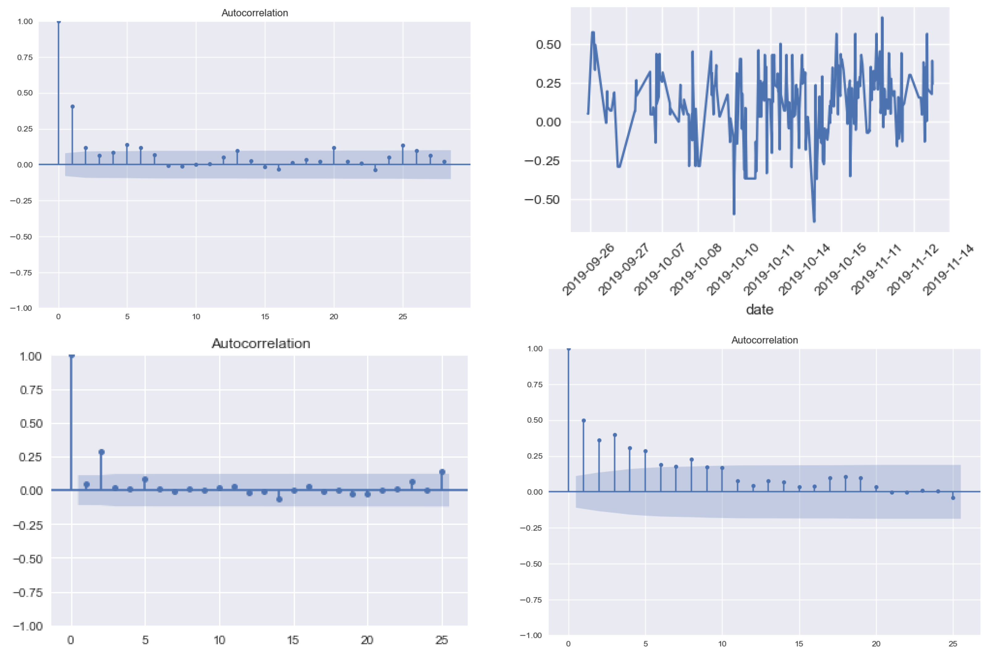
3.2. Popularity and Sentiment Metrics

FinScience retrieves content from the web: about 1.5 million web pages are visited every day on 35,000 different domains. The content of these pages is extracted, interpreted, and analyzed to identify valuable information and sources. The advantage of this approach in web analysis is that it can intercept any kind of topic: it gathers data and information spread by companies, news sources, and through social media.

The data gathering phase involves the collection of data from different web sources: websites, social network pages, news, and blogs. Web urls are conveyed in the database through social media networks such as Twitter, Reddit, Stocktwits, etc. Through the use of blacklists that are constantly kept up to date, data sources that are considered spam or unreliable are removed. After this first phase of data collection, contents are extracted from web pages and preprocessed via a first level of data cleansing to remove “noise” (nonrelevant information) and via the extraction of the main body: this is the input to the next phase of data processing.

At this stage, natural language processing (NLP) methods are carried out. Contents collected during the data gathering phase are subjected to an NLP analysis that allows to identify objects (companies, people, locations, topics, etc.) disseminated and discussed on the web. The DBPedia ontology is used and its named entity recognition (NER)—automatic annotation of entities in a text—is able to associate pieces of text to members of the abovementioned ontology. The ontology is based on the DBpedia Knowledge Graph, which encompasses cleansed data from Wikipedia in all languages. Over the years, such ontology evolved into a successful crowd-sourcing effort with the DBpedia community continuously contributing to the ontology schema. It now contains about 800 classes, numerous properties, and is cross-domain. Based on this ontology, the entities mentioned are identified in the online content and create the structured data that are used as building blocks of the time series associated with what they call “signals” (which can be companies, people, locations, topics, or a combination of them), which enables to identify companies and trends that are spreading in the digital ecosystem as well as analyze how they are related one to each other.

In particular, what is possible to learn from Alternative Data is conveyed and summarized into several metrics, but for the purposes of this research, only the following are taken into consideration:

• Company Digital Popularity measures the level of diffusion of a digital signal on the web. It is obtained by aggregating the diffusion metrics of the news mentioning the company and can take only positive values. The diffusion metric of a news article is quantified by taking into account the number of times the link is shared on social media and also the relevance of the company inside the text. It basically measures how popular a company/stock is among investors.
• Company Sentiment measures the user’s perception concerning the company and can take values in the interval [−1, 1], boundaries included. The sentiment metric of the company on a specific date is represented by a weighted average of the sentiment scores of all news mentioning the company, where the weight is the popularity of the articles.

It is through the use of these two metrics that an attempt will be made to construct a new technical financial indicator.

Popularity and Sentiment Analysis for the Most and the Least Capitalized Companies

In this section, we analyze some features of Sentiment and Popularity metrics for Apple and Jones Soda (simply Jones from here on). These two stocks are the most and the least capitalized companies in the dataset. Our aim is to provide a brief statistical analysis for the time series of these two metrics. Similar results were obtained for each stock in the dataset and are available upon request. As expected,

Table 2. Main statistics for Popularity and Sentiment for Apple and Jones.

Stat.	Apple		Jones
	Pop.	Sent.	Pop.	Sent.
Mean	$0.259\times {10}^6$	0.072	96.844	0.010
St.Dev.	$0.173\times {10}^6$	0.095	267.536	0.242
Skew.	3.437	−0.579	6.765	−0.447
Kurt.	20.309	0.852	66.113	0.002

confirms that an more capitalized company is more popular than a less capitalized one among market operators (i.e., the agents talk more about Apple than Jones). Moreover, the higher Sentiment expected value for Apple denotes that the most capitalized has a good reputation in the considered period (i.e., the Apple news generally improves its public image). It is worth noting that the negative sign of the skewness for Sentiment denotes a low number of strongly negative news even though the majority of them have been positive, leading to a positive mean.

From Figure 3 and Figure 4, the paths of Sentiment and Popularity seem to suggest a stationary behavior in all cases. To further investigate this fact, we consider an augmented Dickey–Fuller test. The null hypothesis is the unit-root against a trend-stationary alternative hypothesis. The p-value for both metrics and both stocks is strictly smaller than 5%, suggesting a stationary behavior. The highest p-value (0.000485) is obtained for the Jones Sentiment.

Both figures report also the autocorrelation functions. At least one lag is statistically significant, denoting an autoregressive dependence structure for these two metrics. In all cases, the first lag is always significant, except for the Jones Popularity that shows a significant nonzero second lag.

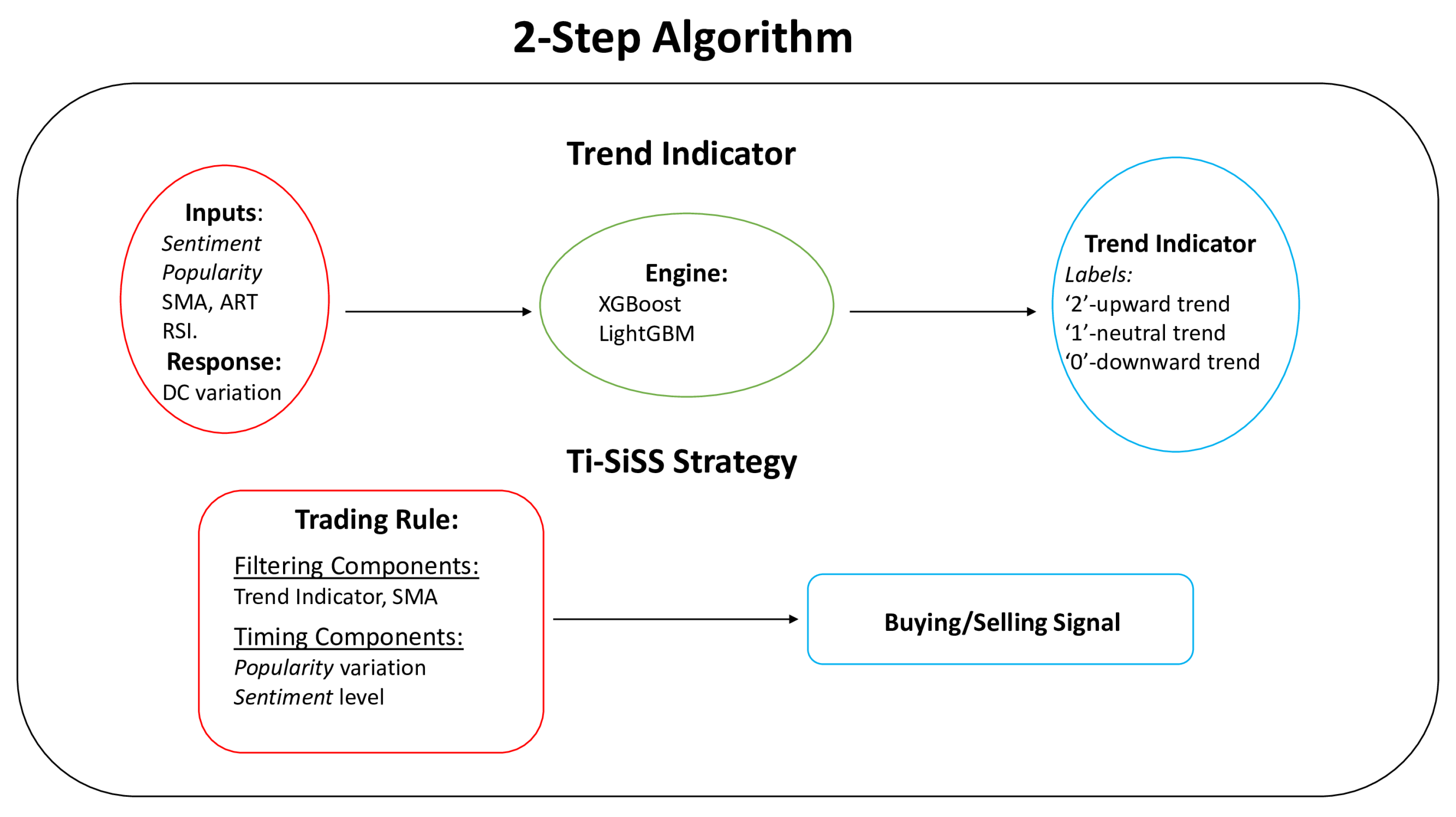
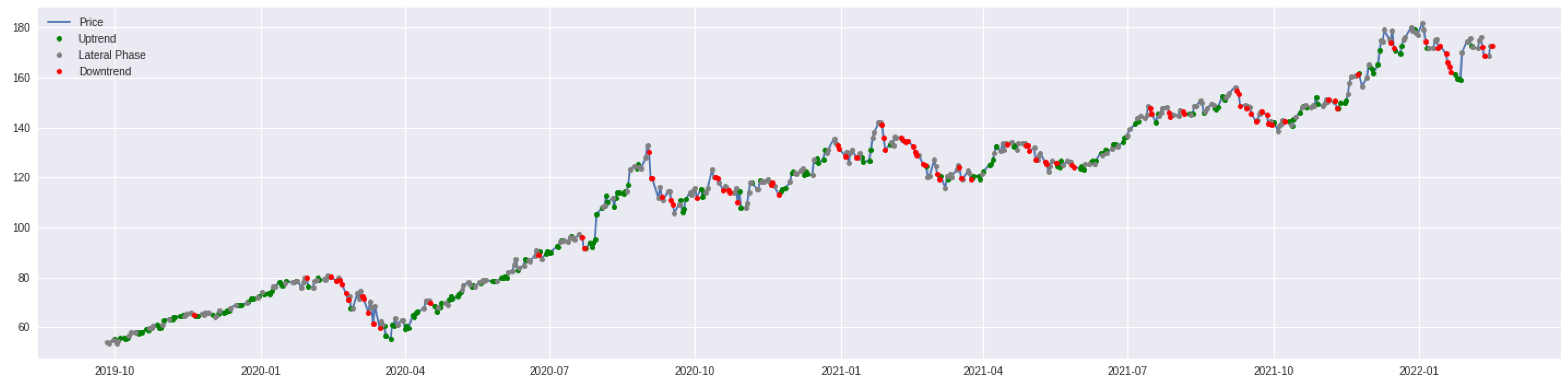
3.3. Trend Indicator

The issue that this research has to face is a classification problem that can be solved through a supervised approach since price directions (creating trends) can be categorized into bullish, bearish, and sideways movements.

3.3.1. Preprocessing Phase

Generally, a common and widely used technique to detect the trend of prices is to calculate simple returns and then investigate the sign of each daily return to asses the price movement. However, this procedure would be too granular, making the labels too sensitive and therefore losing sight of a slightly longer-term trend (weekly), which is quite useful information in trading.

Therefore, in order to better catch the weekly trend of prices, we decided to use a traditional financial indicator in a new, unusual way: the Donchian Channel. However, not all the three lines of this indicator are necessary for detecting a trend and therefore we use only the Upper Channel (UC): it is shifted back in time for the number of input periods to perfectly overlap to the prices, and then its daily variations are taken and saved in a new dataset column. In this way, since the top line of the Donchian Channel is a broken line, it makes it possible to detect the sideways phases that will have a daily variation equal to zero. Therefore, by exploiting the signs of the returns of the UC, it is possible to assign to each day a label describing the kind of movement made by the price, and the result is as in Figure 5, where green dots represent upward price movements, red dots are downward ones, and gray dots represent the lateral phases.

However, our goal is to create predictive models and, therefore, the data we are really interested in are not the label at time t, but rather the label at time $t+1$. For this reason, we create a new column, called Target: this column is nothing more than the result of moving back one period in the column containing the labels. In this way, at each time instant we will have all the data corresponding to that day (which will make up the set of explanatory variables) and the label data of the next day (which will be our response variable, i.e., the output). Thus, in the training phase, the model will take as input the set of explanatory variables, and with them it will try to predict tomorrow’s label, it will check the result, and, in case of discrepancy, it will adjust the parameters.

3.3.2. Trend Indicator Creation through Python

First of all, using the Python package XGBoost (2022) it is necessary to tune the hyperparameters to find the best possible combination and therefore to fit to the data the best possible model. The first parameters to be set among the following possible values are the number of boosting rounds, boosting learning rate, and the learning objective:

• n_estimators: (50, 100, 200, 300, 500, 1000, 2000).
• learning_rate: (0.05, 0.10, 0.15, 0.2, 0.25, 0.3).
• objective: (multi:softprob, ’multi:softmax).

Once these primary hyperparameters are chosen, we also need to set the ones controlling the overfitting of the model, namely, gamma (that encourages the tree pruning if the gain of the branch taken into consideration is lower than the prespecified values of $\gamma$) and the maximum depth of each base learner:

• $\gamma$: (0, 0.1, 0.2, 0.3, 0.5, 1).
• max_depth: (5, 10, 15, 20, 25, 30, 50, 100).

Therefore, after this hyperparameters tuning, the resulting XGBoost model is

XGBClassifier(objective= ’multi:softprob’,n_estimators= 100,
learning_rate= 0.15,gamma= 0,max_depth= 10,random state= 0)

Regarding the LightGBM model, run through the Python package LightGBm (2022), the reasoning is pretty much the same as the one just made for XGBoost, and the hyperparameters to tune with the corresponding possible values are:

• n_estimators: (50, 100, 200, 300, 500, 1000, 2000).
• learning_rate: (0.05, 0.10, 0.15, 0.2, 0.25, 0.3).
• max_depth: (5, 10, 15, 20, 50, 100).
• subsample_for_bin: (5.000, 10.000, 100.000, 200.000, 300.000, 500.000).
• min_split_gain: (0, 0.1, 0.3, 0.5, 1).

Hence, the final best LightGBM model is the following one:

LGBMClassifier(objective= ’softmax’,n_estimators= 300,learning_rate=
0.3,max_depth= 15,subsample_for_bin= 200,000,min_split_gain= 0,random
state= 123)

Now that the best models are defined, we need to place our attention on the kind of data that will be the input of these models. All the most important features upon which all the others are constructed (i.e., adjusted close prices, popularity, and sentiment) are time series: this means that the order of the data is fundamental. Therefore, it is not possible to split them randomly into training and test set because, in this way, you would lose the original order and consequently also the very meaning of the data themselves. Therefore, for each title we take the first 90% of the series as training set and the remaining 10% as test set (these extreme percentages are chosen due to a limited length of the time series data, approximately 3 years): in this way, the intrinsic meaning of the series is maintained for both sets.

However, both XGBoost and LightGBM, when taking an input, return the predictions for the whole test set at once but we know that the further we move into the future with predictions, the less accurate they will be. For this reason, both models are implemented with the so-called rolling technique. This procedure consists of starting with the entire dataset, dividing it, as previously specified, into training and test sets, defining a number of days in the future for which we want the predictions (just one day, i.e., the prediction of tomorrow), and then iteratively performing the following steps:

1.

Use the entire training set for train the model.

2.

Use the trained model to make predictions for the entire test set.

3.

Extract and save the first prediction (i.e., the prediction of tomorrow).

4.

Add the first data point of the test set to the training set.

5.

Go back to step 1 and continue until there are no more data points in the test set.

Hence, both models are embedded in such rolling algorithm to have, every day, the best possible prediction (full code available in Appendix A: Algorithms A1 and A2).

3.3.3. Model Selection and Results

It is probable that not all features have the same relevance and importance within models: some may be irrelevant and may not add valuable information to how much there already is. Therefore, it is also important to perform another kind of tuning, which is also referred to as feature selection. In fact, for improving the capability of XGB or LGBM to make predictions, to speed up their running time and to avoid overfitting, it is crucial to give them as input only those attributes that actually give them gain, excluding the others, to prevent the models from “wasting time” evaluating unnecessary and useless features.

Therefore, the attributes used for creating technical indicators (e.g., adjusted high, low, and open prices) are excluded a priori, and then several combinations of inputs are tested for both XGB and LGBM over the sample dataset, namely:

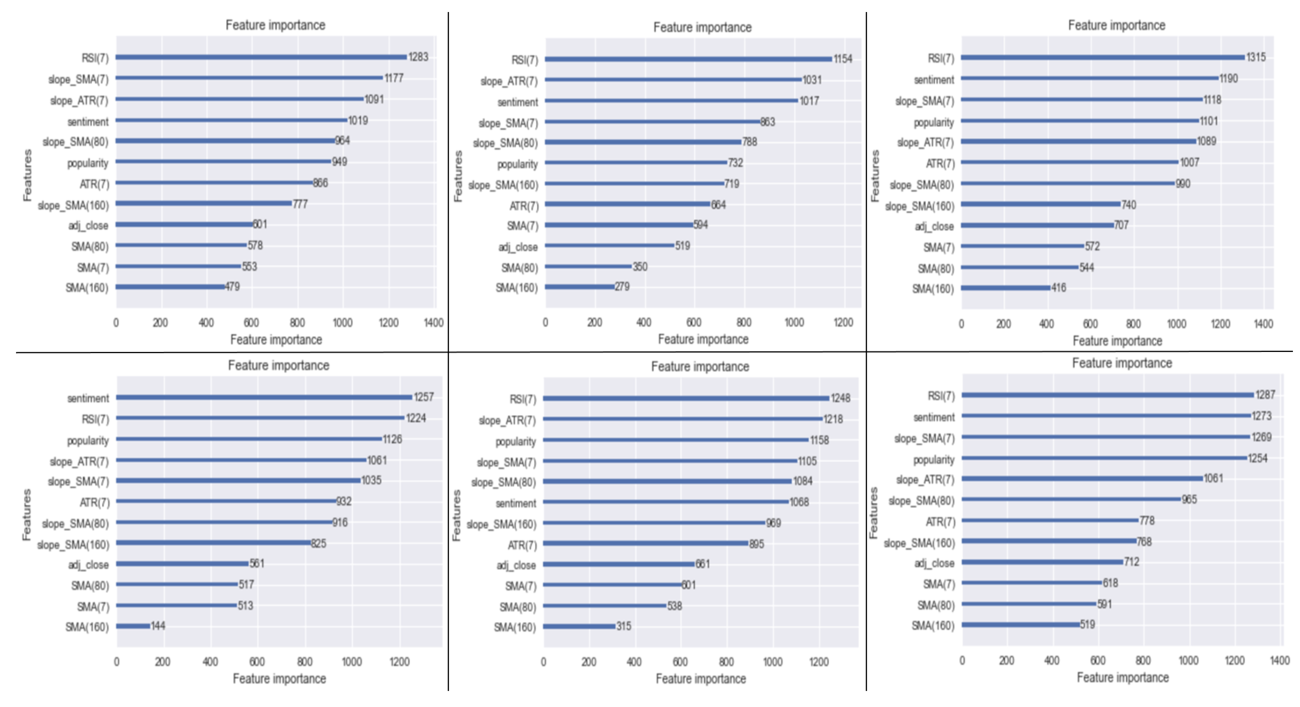
• Model 1: model with all the inputs; closing price, sentiment and its variations, popularity and its variations, SMA(7) and its slope, SMA(80) and its slope, SMA(160) and its slope, ART(7) and its slope, RSI(7) and its slope, Labels${}_t$.
• Model 2: model with all the inputs except for the point value of the simple moving averages (but maintaining their slopes); closing price, sentiment and its variations, popularity and its variations, SMA(7)’s slope, SMA(80)’s slope, SMA(160)’s slope, ART(7) and its slope, RSI(7) and its slope, Labels${}_t$.
• Model 3: model with all the inputs except for the point value of the simple moving averages (but maintaining their slopes) and the variations of sentiment and popularity; closing price, sentiment, popularity, SMA(7)’s slope, SMA(80)’s slope, SMA(160)’s slope, ART(7) and its slope, RSI(7) and its slope, Labels${}_t$.
• Model 4: model with all the inputs except for the variations of sentiment/popularity; closing price, sentiment, popularity, SMA(7) and its slope, SMA(80) and its slope, SMA(160) and its slope, ART(7) and its slope, RSI(7) and its slope, Labels${}_t$.
• Model 5: model with all the inputs except for any value related to the metrics; closing price, SMA(7) and its slope, SMA(80) and its slope, SMA(160) and its slope, ART(7) and its slope, RSI(7) and its slope, Labels${}_t$.

Looking at the average accuracies obtained by each model over the test sets, the best input combination turned out to be the one represented by Model 4, namely, the one with all inputs but with the sentiment and popularity daily variations (but with their point values). Therefore, both XGBoost and LightGBM with this specific input combination are tested over the entire dataset through a powerful virtual machine provided by Google Cloud Platform (GCP), obtaining the following results.

As can be assessed from

Table 3. Results of XGBoost and LightGBM over the entire dataset.

	XGBoost	LightGBM
Tot. Stocks	527	527
N. Stocks < 33%	8	10
N. Stocks > 33%	519	517
Average accuracy	53.95%	53.64%
Running time	6:15 h	3:30 h

, both models performed better than a random gambler (who has a 33% of probability of guessing price trends, since the three possible scenarios are upward movement, downward movement, or sideways phase) in about 518 stocks over 527. Moreover, both XGBoost and LightGBM have an average accuracy well above the minimum threshold of 33%, both being between 53.5% and the 54%. Therefore, our two models have similar performances in terms of accuracy, but not in terms of speed: in fact, the LightGBM took almost the half of XGBoost’s time for making the same computations and maintaining the same accuracy. Moreover, looking at the following explanatory examples, we can also make further considerations over the prediction capability of these models.

Figure 6 and Figure 7 represent the predicted outcome (green) versus the real one (blue): the bullish price trend has label 2, the sideways phase has label 1, while the downwards movement is labeled as 0. In this way, the graph is least confusing as possible: when the line is down prices are falling, when it is in the middle then prices are lateralizing, and when it is up the prices are also up. However, we know that, when using a predictive model, there always are errors, but it is also true that not all the errors have the same severity. In this situation, there are two main types of error:

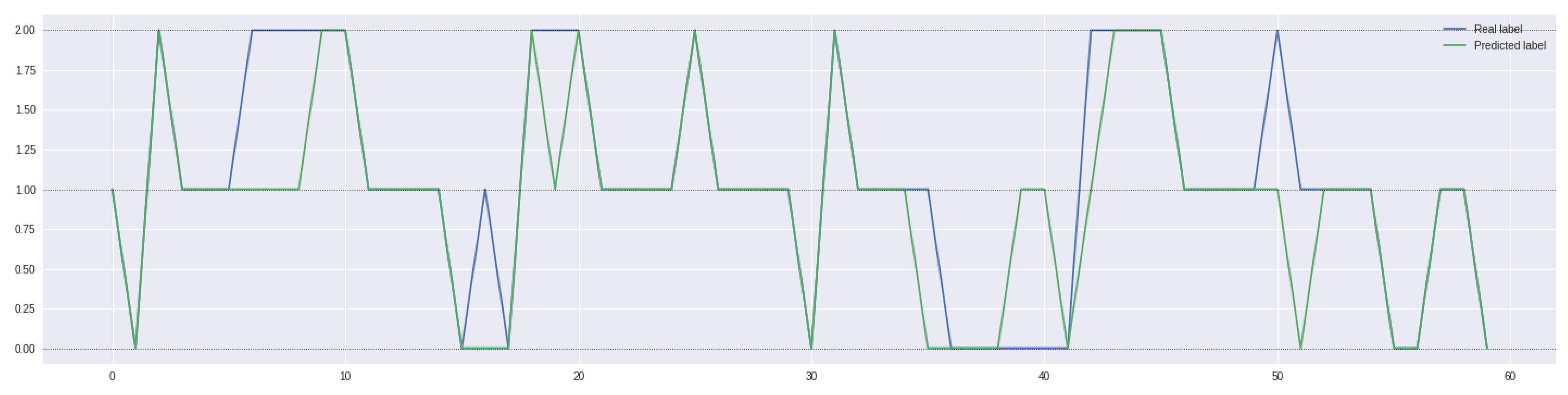
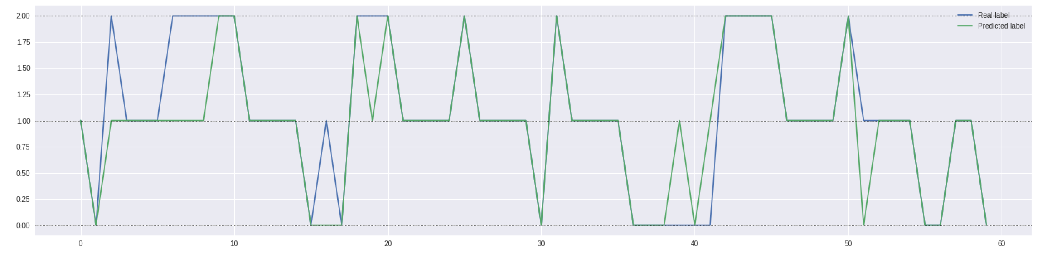
1.

One, representing the case in which the model predicts an ongoing price trend (either positive or negative) and the actual value is a sideways phase (and vice versa);

2.

Another, in which the model predicts an ongoing price trend (either positive or negative) and the actual value is the exact opposite situation.

Moreover, another parameter should also be taken into account: how long a model persists in the error. Unfortunately, the XGBoost, when it makes errors, persists more than LightGBM, as can be seen from

Figure 6 and Figure 7: looking at the period between time step 35 and 45 of both, it is shown how the XGBoost predicts the wrong situation for a longer time than the LightGBM, while the latter immediately corrects the prediction and then anticipates the next bullish trend. The XGBoost corrects its errors slower than LightGBM in the entire dataset.

Therefore, combining all the considerations made so far, we can decree the LightGBM as the best model between the two.

However, what about the metrics? Did they really have an impact within the models? First of all, let us focus only on the best selected model and, to answer to these questions, let us see how the inputs affected the model. Indeed, Figure 8 represents the ranked variables of six different stocks.

Again, these examples of feature importance plots are extendable to the entire dataset and, more in general, at least one metric between Sentiment and Popularity is always in the first half of attributes by utility in the model. Therefore, the digital metrics actually played an important role in the construction of our predictive model.

Summarizing, now we have a new financial technical indicator, called Trend Indicator, that has the following characteristics:

• Created through the machine learning model LightGBM;
• Embedded within a rolling algorithm;
• Capable of reaching an average accuracy of 53.64% (much greater than the threshold of 33%);
• Alternative-data strongly dependent.

Now it is necessary to understand how to use this indicator in a trading strategy.

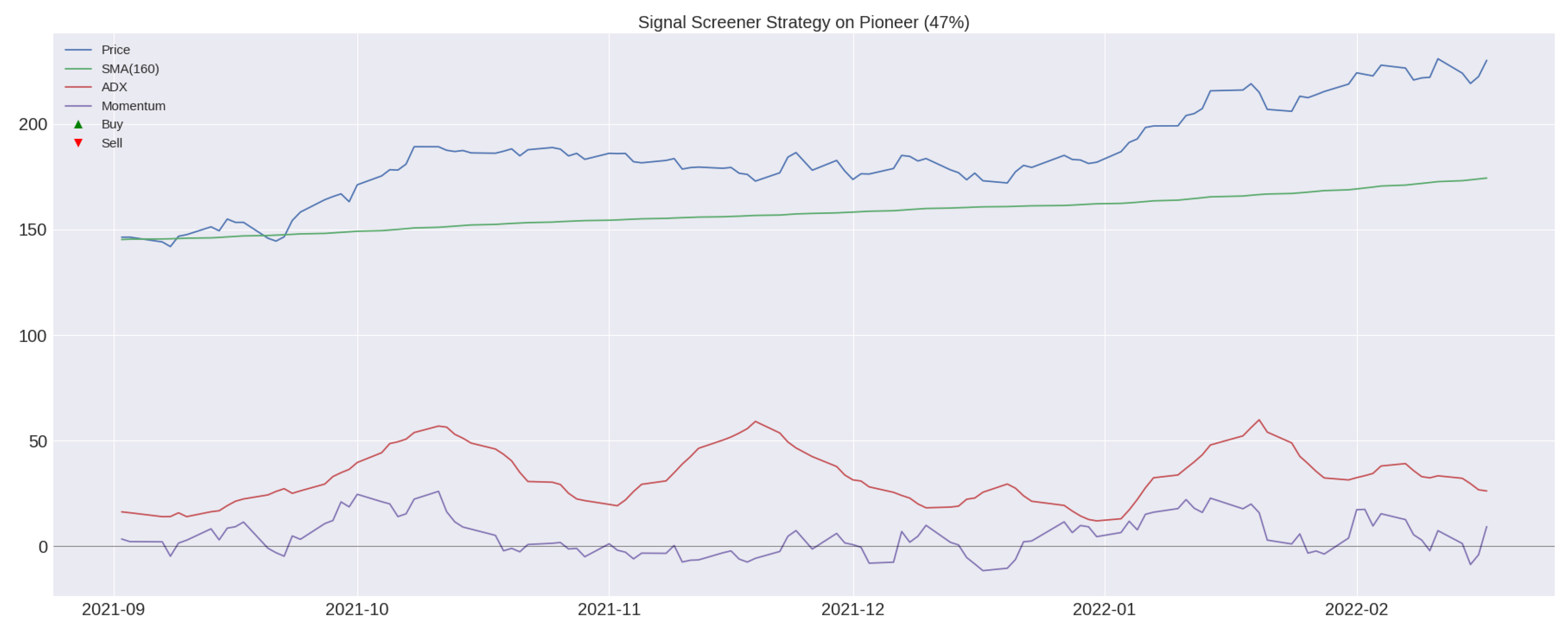
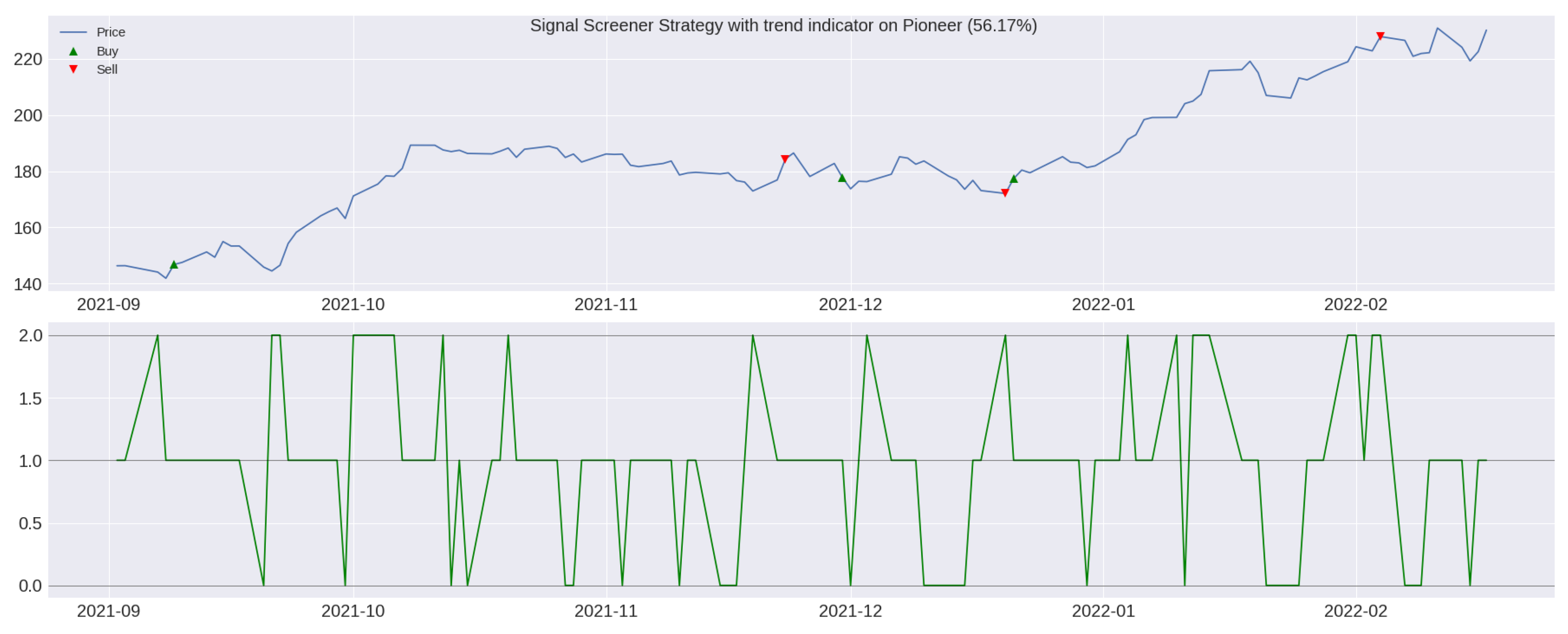
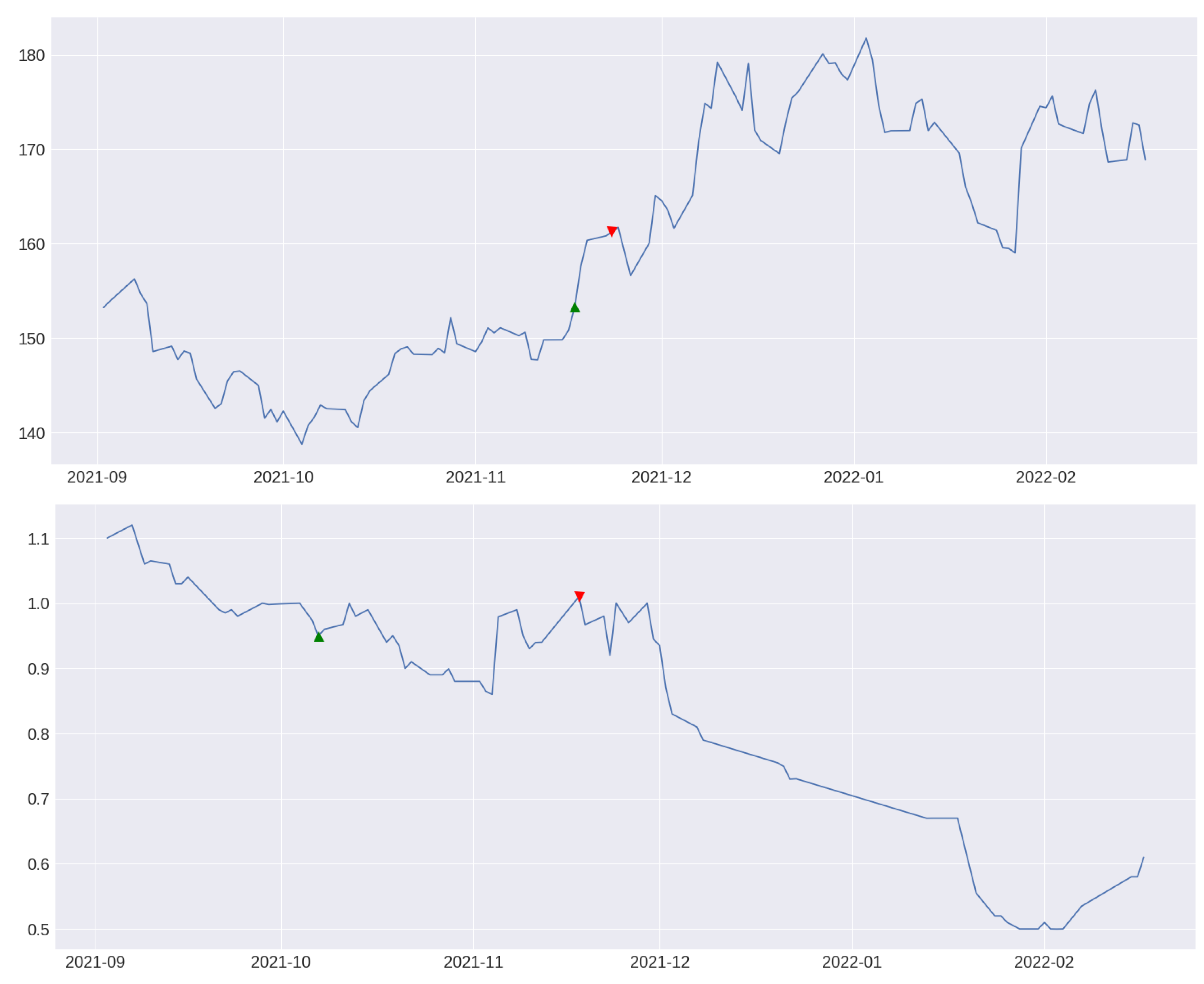
3.4. Algorithmic Trading Strategy: TI-SiSS

To understand whether the Trend Indicator works in a real-world scenario or not, it is necessary to use it in a trading strategy and then evaluate the corresponding results. Therefore, we created two algorithmic trading strategies based on the Signal Screener: this is a feature of the FinScience platform that allows you to view, monitor, and filter sentiment, popularity, and their changes for each security. In addition, so-called alerts can be set up, which are customized notifications based on what the user wants to monitor that make these strategies easily applicable and timely.

The first strategy is called TI-SiSS (Trend Indicator—Signal Screener Strategy, full code available at the end of the paper: Algorithm A3) and, as the name states, it is the one that exploits the information provided by our indicator, while the second strategy is simply the SiSS (Signal Screener Strategy, full code available at the end of the paper: Algorithm A4) to emphasize the fact that it does not use the Trend Indicator.

As shown in

Table 4. Filtering component for both TI-SiSS and SiSS.

SiSS	TI-SiSS
Slope SMA(160) > 0	Slope SMA(160) > 0
Slope ADX Line > 0	Trend Indicator ≥ 1
Momentum > 0

, both strategies are composed of two macro-components, namely, the Filtering component, which identifies among all the possible stocks those that are suitable for our strategies, and the Timing component, which provides some objective rules for opening and closing positions. The filtering component, which is what differs between the two strategies, is composed as follows:

Both strategies require an upward sloping moving average at 160 periods because both of them want to trade in the same direction of the long term and, since the strategies only perform long operations, such long-term must be bullish. Then, the TI-SiSS exploits the Trend Indicator while the SiSS uses ADX and momentum together, since the combination of these two indicators provides the same information as the Trend Indicator, even if our indicator should provide this information a day in advance.

As shown in

Table 5. Timing component for both TI-SiSS and SiSS. $DP{V}_t$ is the value of Popularity at time t; $MA\_DP{V}_t\left(7\right)$ denotes the sample mean of the Popularity over the interval $\left[t-6,t\right]$.

Buy	Sell
$DP{V}_t>MA\_DP{V}_t\left(7\right)$	$DP{V}_t>MA\_DP{V}_t\left(7\right)$
${\displaystyle \frac{DP{V}_t}{DP{V}_{t-1}}}-1\ge 100\%$	${\displaystyle \frac{DP{V}_t}{DP{V}_{t-1}}}-1\ge 100\%$
$Sentimen{t}_t>0.05$	$Sentimen{t}_t<-0.05$

, the timing component, instead, is equal for both the strategies and provides objective rules for buying and selling a stock.

Therefore, both strategies buy when the current value of Popularity is greater than its moving average at seven periods, the change in popularity with respect to the previous available data is at least 100%, and the sentiment is positive. On the other hand, they sell when the same conditions occur, but with a negative sentiment.

Hence, both strategies have the same aim: exploit bullish price movements through long positions. Moreover, by construction, the TI-SiSS and SiSS are easy to compare with each other since they act in the same way and the only difference between them is the way they select the stocks over which they trade on.

Unfortunately, comparing these two strategies is not as straightforward as it could seem. Indeed, while the SiSS has only static computations, making it easily testable in back-test, the TI-SiSS has a structural problem: since the Trend Indicator is based on a machine learning model, it needs as large a history as possible to produce accurate predictions. As a result, TI-SiSS in the first part of the back-test will be neither reliable nor truthful due to the limited training set, while it will perform with the accuracy previously described once the training set is about 80% of the history of each stock. For this reason, it was decided to compare the two strategies by looking only at the returns of the last 20% of observation dates for each stock in our dataset. Clearly, considering only 20 percent of a stock is equivalent to considering just a part for the whole, which is not, and does not claim to be, a complete yardstick, even though it provides a good starting point for making some general assessments on TI-SiSS and SiSS.

Hence, testing the strategies only on the last 20% of observing dates for each stock (test set), we obtain the results in

Table 6. TI-SiSS and SiSS results over the last 20%.

	SiSS	TI-SiSS
Tot. stocks	527	527
N. stocks with trades	134	309
N. stocks with positive returns	104	207
N. stocks with negative returns	30	102
Variance of returns	55.3%	84.02%
Average return	1.98%	3.12%

.

Therefore, for 527 stocks, 134 and 309 stocks trades applied SiSS and TI-SiSS, respectively. Looking at the results, the SiSS had 104 (30) positive (negative) returns, while TI-SiSS had 207 positive and 102 negative results. Therefore, we assess that the TI-SiSS is riskier than the SiSS, as also confirmed by a higher variance of the returns, but this risk is repaid by a higher average gain, rebalancing the whole scenario.

Finally, it is interesting to analyze how the two strategies behave on the same stock see Figure 9 and Figure 10. For this comparison, we cannot use the aforementioned five most/least capitalized stocks since there were no operations of the SiSS in the last 20% of the time period. For this reason, we conduct this comparison on Pioneer Natural Resources Co., (Irving, TX, UAS) which has an average value of market capitalization (56 billion)among the 527 companies in the considered dataset. Then, in this case, TI-SiSS performed better, anticipating the market with the opening of the first trade (the first green triangle) and then achieving a better final return.

Gross and Net Profit Analysis for a TI-SiSS Strategy

We conclude this part by discussing the performances of the TI-SiSS strategy applied to the five most and least capitalized companies. As also remarked above, for this analysis we consider the test set period that is composed of the 20% of observed days of each stock. Therefore, the first date of the test set is around 1 September 2021 for all 527 companies3. In general, for the five most/least capitalized assets we have no more than four trade signals. For example, as shown in Figure 11, we observe only two signals for Apple and Jones, which gives us an overall positive gain.

Using the buying/selling signals for each stock in

Table 7. Gross performances for a TI-SiSS trading strategy for the most/least capitalized companies.

	Operations	Apple	Microsoft	United Health	J&J	Exxon
1st	Buying	100	100	100	100	100
2nd	Selling	105.160	110.076	99.799	104.850	104.717
3rd	Buying	-	-	-	104.850	-
4th	Selling	-	-	-	106.886	-
MDD		0	−7.500%	−0.201%	−3.791%	−0.488%
		Tejon	Entravision	Community Health	Provident	Jones
1st	Buying	100	100	100	100	100
2nd	Selling	99.406	109.144	85.868	97.844	106.316
3rd	Buying	99.406	109.144	85.868	97.844	-
4th	Selling	99.138	104.626	116.883	99.668	-
MDD		−9.302%	−25.926%	−25%	−5.392%	−13.333%

, we construct the corresponding TI-SiSS strategy with EUR 100 as initial wealth. If we consider the five most capitalized companies, the TI-SiSS strategy returns a positive performance in all cases except for United Health asset. The highest gain is achieved for Microsoft (more than 10% of the initial wealth). Table 7 reports the maximum drawdown (MDD) for the performances and we note that the TI-SiSS is able to provide a gain even when there are some strong downward movements in the stock price behavior (for instance, see Microsoft among the most capitalized). For the five least capitalized companies, we have a loss only in two cases, with the highest gain for Community Health, and when comparing the performances with the MDD we observe that, in all cases, our strategy gives much better results.

Table 8. Net performances for a TI-SiSS trading strategy for the most/least capitalized companies. To determine the net performance, we consider 1% of wealth as a multiplicative transaction cost for each buying/selling operation.

	Operations	Apple	Microsoft	United Health	J&J	Exxon
1st	Buying	100	100	100	100	100
2nd	Selling	104.108	108.975	98.802	103.801	103.670
3rd	Buying	-	-	-	102.763	-
4th	Selling	-	-	-	103.708	-
		Tejon	Entravision	Community Health	Provident	Jones
1st	Buying	100	100	100	100	100
2nd	Selling	98.412	108.053	85.009	96.865	105.253
3rd	Buying	97.428	106.972	84.159	95.897	-
4th	Selling	96.193	101.518	114.411	96.798	-

analyzes the performances of the TI-SiSS strategy, introducing a multiplicative transaction cost that is 1% of wealth. The transaction cost is applied for each buying/selling signal. The conclusions in Table 7 are confirmed.

4. Conclusions

Using Alternative Data, we were able to construct a new financial technical indicator, named Trend Indicator, for each stock in the dataset. Alternative Data refers to unique information content not previously known to financial markets in the investment process. Investors, vendors, and research firms use the term to refer to information that is different from the usual government- or company-provided data on the economy, earnings, and other traditional metrics. Alternative Data are big and often unstructured data coming from different sources, mainly digital (i.e., blogs, forums, social or e-commerce platforms, maps, etc.), and whose analysis implies an algorithmic approach, unique expertise, and cutting-edge technology.

Using Alternative Data, FinScience daily publishes two alternative data metrics obtained by applying NLP algorithms such as entity extraction and classification: Sentiment and Popularity. These two quantities were used for the construction of our “Trend Indicator” (for each stock) that leads to the TI-SiSS strategy. To check the profitability of the TI-SiSS, we compared it to the SiSS strategy. The latter provided positive results and is the natural competitor of our strategy. Moreover, we conducted a gross/net performance analysis of the TI-SiSS for the five most/least capitalized companies in the dataset. It is worth noting that TI-SiSS is able to provide a gain even though there are some strong downward movements in the stock price behavior (see, for instance, Microsoft, for which we observed the lowest value of the maximum drawdown while the corresponding TI-SiSS’s gain was the largest one among the five most capitalized stocks). A possible drawback of our trading strategy may be given by the choice of the underlying news: in some cases, it could not necessarily be related to financial topics. Moreover, a possible bias comes from the presence of fake news which might be present on social media.

Further investigation is needed to improve the strategy by including other sources or by testing our strategy on intraday stock data and considering different markets.

References

- Achelis, Steven B. 2001. Technical Analysis from A to Z, 1st ed. New York: McGraw Hill. [Google Scholar]
- Allen, Franklin, and Risto Karjalainen. 1999. Using genetic algorithms to find technical trading rules. Journal of Financial Economics 51: 245–71. [Google Scholar] [CrossRef]
- Ballings, Michel, Dirk Van den Poel, Nathalie Hespeels, and Ruben Gryp. 2015. Evaluating multiple classifiers for stock price direction prediction. Expert Systems with Applications 42: 7046–56. [Google Scholar] [CrossRef]
- Barucci, Emilio, Michele Bonollo, Federico Poli, and Edit Rroji. 2021. A machine learning algorithm for stock picking built on information based outliers. Expert Systems with Applications 184: 115497. [Google Scholar] [CrossRef]
- Bollen, Johan, Huina Mao, and Xiaojun Zeng. 2011. Twitter mood predicts the stock market. Journal of Computational Science 2: 1–8. [Google Scholar] [CrossRef]
- Chen, Tianqi, and Carlos Guestrin. 2016. Xgboost: A scalable tree boosting system. Paper presented at 22nd Acm Sigkdd International Conference on Knowledge Discovery and Data Mining, San Francisco, CA, USA, August 13–17. [Google Scholar]
- Chong, Eunsuk, Chulwoo Han, and Frank C. Park. 2017. Deep learning networks for stock market analysis and prediction: Methodology, data representations, and case studies. Expert Systems with Applications 83: 187–205. [Google Scholar] [CrossRef]
- Duz Tan, Selin, and Oktay Tas. 2021. Social media sentiment in international stock returns and trading activity. Journal of Behavioral Finance 22: 221–34. [Google Scholar] [CrossRef]
- Ellis, Craig A., and Simon A. Parbery. 2005. Is smarter better? A comparison of adaptive, and simple moving average trading strategies. Research in International Business and Finance 19: 399–411. [Google Scholar] [CrossRef]
- Fama, Eugene F. 1970. Efficient capital markets: A review of theory and empirical work. Journal of Finance 25: 383–417. [Google Scholar] [CrossRef]
- Jaquart, Patrick, David Dann, and Carl Martin. 2020. Machine learning for bitcoin pricing—A structured literature review. Paper presented at WI 2020 Proceedings, Potsdam, Germany, March 8–11; Berlin: GITO Verlag, pp. 174–88. [Google Scholar]
- Ke, Guolin, Qi Meng, Thomas Finley, Taifeng Wang, Wei Chen, Weidong Ma, Qiwei Ye, and Tie-Yan Liu. 2017. Lightgbm: A highly efficient gradient boosting decision tree. Paper presented at 31st Conference on Neural Information Processing Systems (NIPS 2017), Long Beach, CA, USA, December 4–9. [Google Scholar]
- Lee, Ming-Chi. 2009. Using support vector machine with a hybrid feature selection method to the stock trend prediction. Expert Systems with Applications 36: 10896–904. [Google Scholar] [CrossRef]
- Levy, Robert A. 1967. Relative strength as a criterion for investment selection. The Journal of Finance 22: 595–610. [Google Scholar] [CrossRef]
- LightGBm. 2022. Python Package. Available online: https://lightgbm.readthedocs.io/en/v3.3.2/ (accessed on 10 October 2022).
- Thomsett, Michael C. 2019. Momentum Oscillators: Duration and Speed of a Trend. In Practical Trend Analysis: Applying Signals and Indicators to Improve Trade Timing, 2nd ed. Berlin: De Gruyter. [Google Scholar]
- XGBoost. 2022. Python Package. Available online: https://xgboost.readthedocs.io/en/stable/python/index.html (accessed on 3 November 2022).
- Yang, Steve Y., Sheung Yin Kevin Mo, Anqi Liu, and Andrei A. Kirilenko. 2017. Genetic programming optimization for a sentiment feedback strength based trading strategy. Neurocomputing 264: 29–41. [Google Scholar] [CrossRef]