Abstract
We develop a novel quantum algorithm for approximating the price of a discrete floating-strike Asian option based on an underlying valuation tree. The paths of the tree are encoded in bit-representation into a qubit register, where quantum state preparation is used to load the corresponding distribution onto the states. We implement the expectation value of the option pricing formula as a composition of the price probabilities, the payout and an indicator function, mapping their respective values to amplitudes of additional qubits. Thus, the underlying no longer has to be discretized into the same bit values for different times, resulting in smaller quantum circuits. The algorithm may be used with quantum amplitude estimation, enabling a quadratic speed-up over classical Monte Carlo methods.
1. Introduction
Due to the progress in developing quantum computers, the research in the field of industrial applications has intensified in recent years. One important branch of industry is the financial sector, in which a number of very complex and computer-intensive applications can be found, e.g., the evaluation of insurance portfolios or the pricing of structured financial products. Accordingly, the use of a quantum computer for both applications is investigated, in e.g., Egger et al. (2021). In the field of derivative pricing, the article by Rebentrost et al. (2018) is considered to be one of the first influential works. They present a way to price plain vanilla and Asian options in a Black–Scholes framework using quantum computing. In theory, quantum computers have the potential for a quadratic speed-up with respect to the number of computational steps compared to classical Monte Carlo methods used for option pricing. Because current quantum hardware is still small, many quantum algorithms are of hybrid character, meaning a mixture of classical computer applications and quantum computations. Therefore quantum speed-up must still be shown. Stamatopoulos et al. (2020) focus their research on the possibilities and performance of the currently available noisy intermediate-scale quantum (NISQ, cf. Preskill (2018)) hardware to price multi-asset and path-dependent options. Especially latter ones are subject to further research, as they are harder to price than path-independent ones and therefore more promising for the speed-up that quantum computers promise. Likewise, in a Black–Scholes framework, Chakrabarti et al. (2021) present an algorithm which precomputes standard normal distributions into quantum states and uses affine transformations to obtain the asset’s path-dependent return distributions. In addition to this new method, they also derive bounds on required resources for established quantum algorithms in finance to reach a practical quantum advantage. Another approach, followed by Miyamoto and Kubo (2021), is to solve partial derivative equations (PDE) for option prices by using the finite difference method. They define grit points for the logarithmic value of the underlying at maturity and calculate its value by using a discretized operator based on the PDE to describe the evolution. The quantum computer is used to calculate the resulting systems of equations. Pricing multi-dimensional derivatives with the help of discretizing their price PDEs is a method Kubo et al. (2022) use as well. The novelty being that a variational quantum algorithm (VQA) is used to calculate the development of the underlying. This allows obtaining helpful results even for small-scaled quantum computers with only a few qubits available. To demonstrate the possibilities of the currently small quantum computers, Woerner and Egger (2019) made an application study using real hardware to calculate the risk measures of a financial portfolio. Since the resources of current quantum computers are quite limited, simplifications in the financial models are necessary. One such method is the principal component analysis where a quantum alternative exists as well. Martin et al. (2021) use a Heath–Jarrow–Morton framework for modeling forward rates and in doing so show how the model is adapted to the quantum computer. The application of a quantum gradient estimation algorithm to calculate financial indicators of sensitivity, so-called Greeks, is illustrated by Stamatopoulos et al. (2022). They present different approaches and investigate their complexity with respect to the requirements of quantum computers. We adopt a similar approach as in Blank et al. (2021). They consider a discrete stochastic process and develop a quantum algorithm to calculate its characteristic function. This derives the whole probability distribution for the stochastic trajectories resulting in a valuation tree approach for pricing derivatives. The work by Vazquez and Woerner (2021) also has to be mentioned, who show an efficient way to prepare quantum states when employing amplitude estimation and present their findings on a Heston model for option pricing using real hardware.
The presented research shows that quantum computing becomes more and more relevant for financial questions as the development of the hardware progresses. Currently, simulators of quantum computers and real quantum computers are used to make first experiences with this technology and learn how classically well understood problems can be solved with the help of the quantum technology. In our work, we aim at contributing to this development in this exact way. As a use case, we choose an Asian option, which puts some challenges to pricing due to its path-dependence. Asian options, sometimes equivalently called traded average price options (TAPOs), are derivatives that are commonly used in the energy and metal sector for hedging purposes. Using this as an example, we show how the classical approach of a valuation tree can be decomposed into three modules in order to be adapted to the requirements of a quantum computer. Each of the three calculation steps individually can already be evaluated on real quantum computers. As the hardware is still not powerful enough for the whole problem at once, our evaluations are performed with the help of a simulator for a quantum computer. Nevertheless, our results show that in the future, the whole algorithm will be applicable on a real quantum computer. The decomposition of the algorithm comprises the calculation of the underlying’s probability distribution, the evaluation of the payoff and the encoding of an indicator function.
This new approach results in substantially less qubits used per time step. By encoding the underlying as probabilities and not in a bit representation, the derivative can be priced in a very efficient way. The paper is structured as follows. After presenting the mathematically formulated problem and the general ideas of our algorithm to solve this problem in Section 2, we give a quick overview on the underlying techniques used on a quantum computer in Section 3. Afterwards, in Section 4, we present our implementation in detail. We finish our research by illustrating the results of the entire algorithm for different problem sizes on a quantum computer simulator in Section 5. The paper closes with a discussion of our work in Section 6.
2. Problem and Algorithm
Let be an underlying, stochastic security price process in a financial model with arbitrary, but known, distribution. Assume the financial model to be free of arbitrage and that there exists some equivalent martingale measure (EMM) . Additionally, let the first moment of exist (at least under ). Then, the fair price of a discrete floating-strike Asian option with maturity T and n time steps is given by (see, e.g., Korn et al. (2010))
where is the risk-neutral EMM, is a suitable filtration, and is the deterministic discount factor at time t. For simplicity, we assume a zero-interest situation, for all . Additionally, as only the risk-neutral measure is relevant for our computations, for clarity, we may assume that for some physical measure . To summarize, our objective is the computation of
Be aware that a fixed-strike Asian option can be priced with the upcoming algorithm as well as it is less complex using a constant strike K instead of the variable .
General Idea
Recall that the dynamics of the underlying security are known. We will now approximate this security by using a valuation tree with two distinct discretizations. The first discretization will be completed with respect to time, where we will only use the time steps needed for the Asian option, using the index i to refer to this for the remainder. The second discretization has to be completed in the range of our underlying for each respective time step. Here, at time , the underlying will only be able to equal a finite amount of values , where is the number of discretization points, i.e., nodes. Even though the discretization may change depending on , we write k instead of for notational simplicity. Generally, the index k will be used to refer to all discretizations that do not refer to time. We combine different layers by defining transition probabilities to approximate the continuous underlying.
One example for a valuation tree would be the Cox–Ross–Rubinstein model by Cox et al. (1979), where a binomial tree is used to approximate a log-normally distributed underlying. It has to be stated that for our implementation, we are not only limited to binomial trees; all scenario trees, with discretely many edges, may be employed.
We denote each possible distinct path through the valuation tree with and . Consequently, there exist paths. Let be the number of qubits needed to represent all possible paths. If , we may set the upcoming probability of the respective additional paths for . This now enables us to approximate Equation (1) via
where the different functions are accordingly defined as
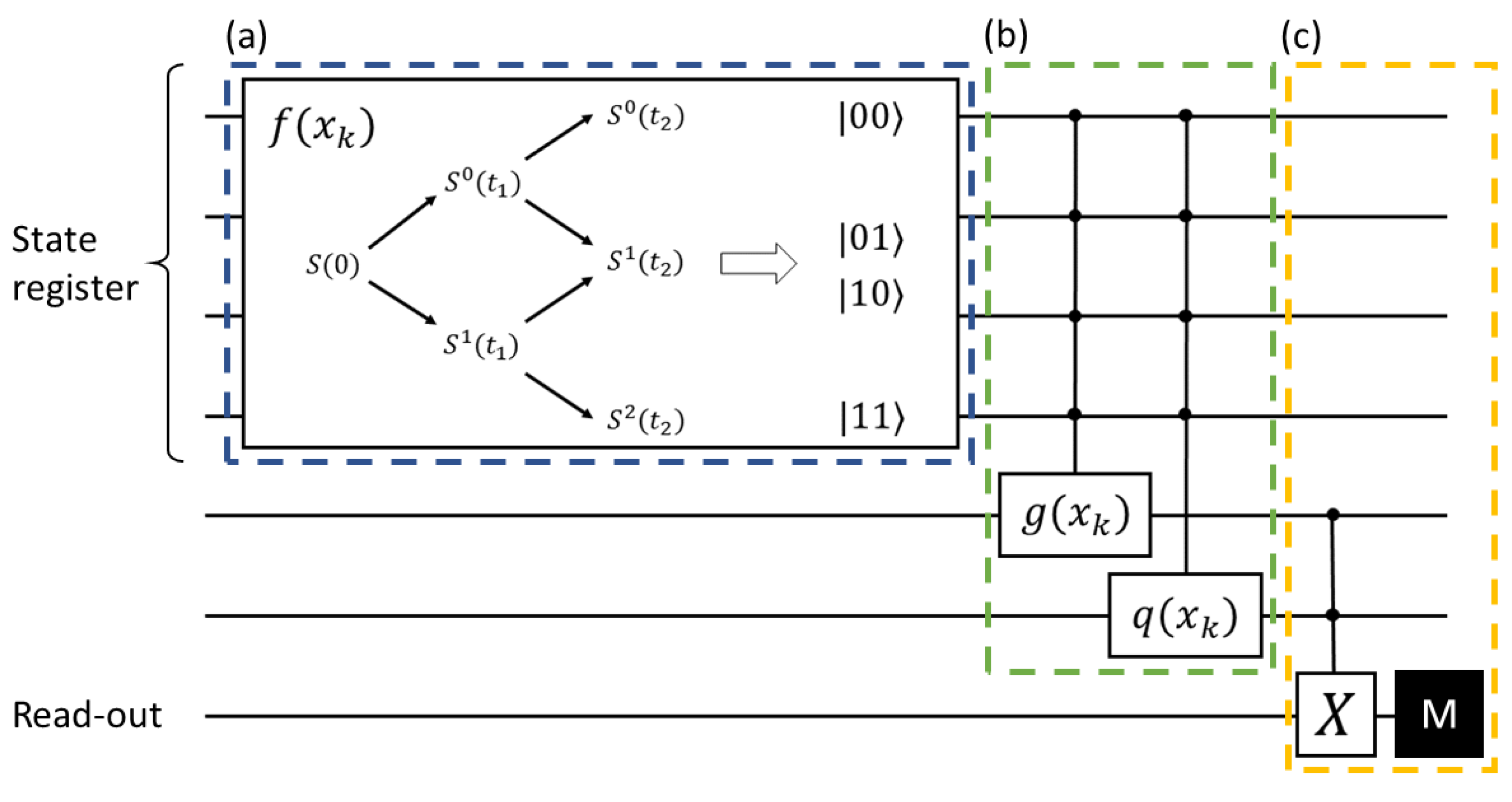
We present a visualization of the proposed algorithm in Figure 1. We start by computing the possible values of the underlying in our scenario on a classical computer. Then, an N qubit state register is allocated to represent all paths of the underlying that may possibly occur during an evolution period comprising n time steps, as shown in Figure 1a. The qubits’ weights (amplitudes) are prepared to correspond to the respective asset probabilities denoted by the function f. The functions g and q for the payoff are then implemented separately as unitary transformations controlled by the N qubit state register in Figure 1b. In Figure 1c, they are recombined to calculate the scaled Asian option price, which can be read out by repeated measurements. A post-processing step ensures correct re-scaling. Using quantum parallelism, the option payoffs of all paths can be evaluated simultaneously.
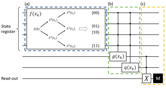
Figure 1.
A visualization of the upcoming algorithm as a quantum circuit model. The horizontal lines represent the used qubits. The black circles show the function’s dependence on the respective qubits. (a) The given valuation tree is mapped to a qubit register, encoding in the qubit states the asset’s path values . The underlying’s path probabilities are associated with the qubit’s state probabilities. (b) Depending on the path, the payoff and indicator function are implemented on different qubits. (c) The functions are combined on a read-out qubit and finally measured.
3. Quantum Programming
3.1. Qubits
A qubit is a two-dimensional vector with the condition that . We may write the qubit in Dirac notation as
where the index denotes the specific qubit, are the computational basis states and represents a combination of them. We call a and b the amplitudes of their respective states, and the probability of measuring the qubit in the respective state is given by the squared, absolute value of the amplitude.
A quantum register consists of N qubits and may be represented as the sum of its computational basis states
Here, |k⟩ is the binary representation of integer k. For additional clarity, we sometimes write the number of qubits as an upper index, e.g., we write for an N-qubit register with each qubit being in basis state |0⟩. The condition on the amplitudes for a quantum register accordingly changes to .
3.2. Quantum Circuits
A quantum circuit is a model for quantum computations where a computation is a sequence of gates applied to a set of qubits akin to a bit-based circuit used in classical computing. Quantum gates are algorithmic steps to the qubits and mathematically expressed by applying unitary matrices to the vector representation of the qubits. In this paper, we will primarily make use of the Hadamard gate H used for creating an equal superposition. Moreover the X-gate which switches amplitudes, the -gate and their conditional variants are used respectively. They are defined as:
The controlled operations act on two qubits and are therefore represented by matrices. The included single-qubit transformation U is only applied to the target qubits if the control qubit is found in state 1.
3.3. Measurement
Determining the state of a qubit is accomplished by repeated measurements. In quantum computing, we generally refer to measurements with respect to the computational basis states, but theoretically, other measurement bases are possible. When a qubit is measured, its probability of being in state |1⟩ is given by
where we defined a new notation for easier readability. Here, U is the matrix corresponding to the used quantum circuit. It is now easy to see that applying the operator for will generate the result of . Because of this, we will restrict ourselves to the use of -gate for ease of understanding. Circuit optimizations employing complex-valued rotations may be possible.
3.4. Arithmetics with Amplitudes
Almost every quantum circuit is built up of smaller subcircuits, each implementing a different part of the computation. It can generally be distinguished between two different approaches of data encoding when studying these subcircuits: an amplitude-based approach and a bit-based approach. The bit-based approach encodes data in multiple qubits, where after measurement, each qubit can be viewed as a bit (due to it collapsing to either 0 or 1), similar to classical computing. The amplitude-based approach encodes data as amplitudes, making the information available by measuring the number of times a certain state happens. By doing this, there is no restriction on some discretization that has to be chosen for the bit-encoding. Hence, we may encode arbitrary values of our underlying for different time steps and use arithmetics on an amplitude level to combine them precisely. Therefore, we are quickly going to state one of the main results used for the presented algorithm, the addition of amplitudes as presented in Vazquez and Woerner (2021).
For n operators generating the state
we are able to construct quantum circuits where the probability of our target qubit being in state |1⟩ is given by
We can also implement a subtraction of amplitudes by employing another -gate. In other words, for quantum circuits and implementing a qubit to be measured in state |1⟩ with a probability of and , respectively, we may construct with
Note that we can retrieve the needed addition or subtraction by proper rescaling of the resulting probability. An example circuit for is given in Figure 2.

Figure 2.
Visualization of the quantum circuit implementing the operator for calculating the difference of two functions implemented by the operators . Note that both functions may also depend on some state register if needed. The last Hadamard application uncomputes the qubit .
4. Quantum Algorithm
4.1. Encoding the Paths
For the implementation of the algorithm on a quantum computer, we have to find a mapping of all possible paths through the valuation tree to a qubit register. The employed qubit register will be referred to as the state register for the remainder of this article, and it consists of N qubits. Assume that in our valuation tree, all nodes of the previous level are connected to the nodes of the current level. One example of such a mapping would be to represent the possible values of with a state (in binary representation) of a qubit register. Doing this for all time steps , we may combine them to denote the entire state register by , where are the computational basis states. Each can then be understood as a path taken through the approximating tree consisting of the individual .
In the following, we will present how each of the functions in Section 1 may be implemented as a quantum circuit with a single path given as an input state. If properly constructed, we can eventually set our state register |s⟩ as a superposition over all the paths to obtain the simultaneous computation.
4.2. Encoding the Probabilities
Assume we have an operator P that does the following transformation to our state register:
Then, the path probabilities are directly encoded in the amplitude of their respective state, and operators mapping from the state register have the needed probability. Constructing this operator P as a quantum circuit is generally referred to as quantum state preparation, and for arbitrary functions f, it requires an exponential number of gates (cf. Shende et al. 2006; Plesch and Brukner 2011). Finding operators efficiently implementing P is a widely researched problem with various algorithms available, e.g., Grover and Rudolph (2002); Zoufal et al. (2019); Holmes and Matsuura (2020), and Zhang et al. (2021). Therefore, let us assume an appropriate operator to be given.
4.3. Encoding the Payoff
As previously explained, the algorithm uses the classically computed for the implementation of the option value. To encode them on a qubit amplitude, we need to ensure that all values are in . This can be completed by using an appropriate scaling technique. For this purpose, let and define the transformation
We first focus on implementing the mean of our underlying. Using uniformly controlled rotations, a technique introduced by Möttönen et al. (2004) and further developed by Shende et al. (2006), we may construct operators implementing
Employing Equation (10), we can construct an operator with
where is the amount of additional ancillary qubits needed. These are qubits that are only used for auxiliary purposes and are not directly depending on the input. Often, they are reusable at a later point when employing an uncomputing process.
Furthermore, using Equation (11), , and two additional qubits and , we are able to build an operator G with
Note that we constructed G in such a way that all the necessary information is loaded on state . Combining G with the probability loading operator P from (12), we obtain the following probability of measuring the success state :
where N is the number of qubits in , and for the last equality, we used Equation (13). We may now retrieve by the appropriate re-scaling.
Let V be another operator implementing some amplitude . We want to multiply with the previously constructed by, for example, employing a Toffoli gate. This introduces an error term of . We can subtract this error term at the cost of another factor of by employing an additional amplitude subtraction, which accordingly yields
We will use this method to combine with the positive part introduced in the next part.
4.4. Encoding the Positive Part
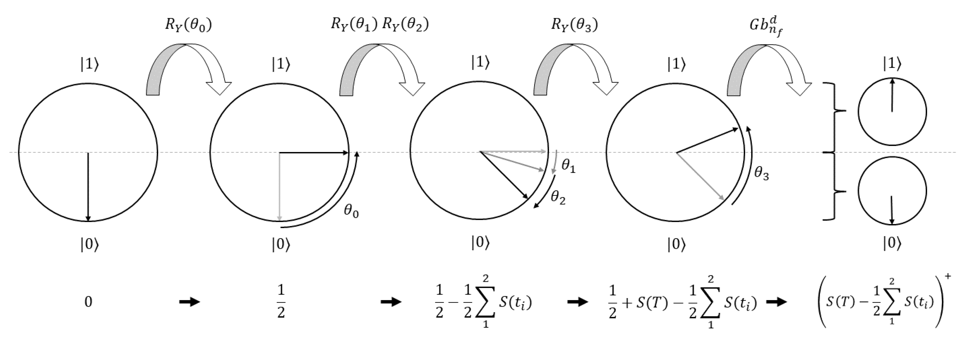
Remember that all the constructed values are encoded in probabilities and not in qubit states. Because of this, accessing them is difficult and generally completed using measurements. This complicates a possible implementation of the positive part. Nevertheless, Koppe and Wolf (2022) showed how to construct a quantum circuit that implements the positive part depending on some input angle of an -gate. We may employ this technique by carefully encoding the needed option payoff as the final angle of a series of rotations. A visual representation of our encoding and how this constructs the needed input angle is shown in Figure 3. To be more precise, we construct a circuit with approximation level D implementing
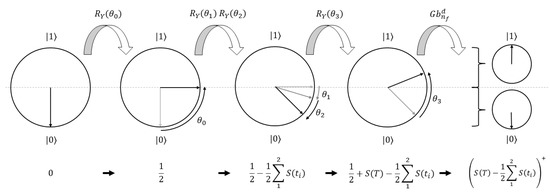
Figure 3.
Representation of the quantum algorithm implementing the positive part of the value at maturity for . As the -gate only rotates about the Y-axis, we can illustrate the employed rotations by showing the relevant 2-dimensional Bloch sphere of the used qubit. The used rotations are shown above, and the corresponding values are shown below. In the last step, the employed gearbox circuit sets a qubit in state |1⟩ for angles above and in state 0 for angles below , ultimately implementing the needed function as shown in Equation (22).
The right-hand side of Equation (19) contains the limit value of a Fourier series
For the evaluation of the probability, the order of the Fourier expansion has to be decided for being able to implement a simultaneous computation. Due to the periodicity of the right-hand side, only cosine terms are needed. We denote the resulting circuit we employ by . As the circuit employs -gates, we may use the fact that to implement the angle used for Equation (19) as a sum of individual angles with
where , with , being a scaled-down version of . In other words, each asset value now corresponds to a rotation resulting in
4.5. Concatenate Circuits and Resulting Computation
Let us now concatenate the above circuits as a new circuit Z combining their respective target qubits using a multi-controlled X-gate on a new target qubit we denote as . The resulting probability is then given as
When executing the quantum circuit Z multiple times and counting the number of times state was measured, we obtain an estimator for the probability and may retrieve an estimator for the fair option price by rescaling the result as
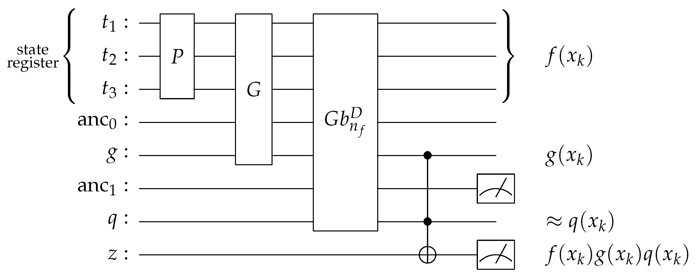
The complete quantum circuit is presented in Figure 4.

Figure 4.
A visual representation of the quantum circuit to price a floating-strike Asian option for . For and , the probability of measuring them in state |1⟩, given the state register is in state , is shown at the right-hand side. We abbreviated the ancillary qubit registers needed for the circuit parts G and with and , respectively. Note that, as described in Equation (22), the is approximated.
4.6. Amplitude Estimation and Quantum Speed-Up
The quantum speed-up for computing expectation values derives from the use of quantum amplitude estimation (AE) introduced by Brassard et al. (2000). Given an operator Z implementing the transformation
AE allows us to estimate the probability of the state being measured with a convergence speed of , where is the number of circuit executions. Montanaro (2015) presented that if this amplitude is carefully constructed to represent an expectation value, this estimator converges faster than classical Monte Carlo methods converging with . By construction, our quantum circuit is compatible with AE; therefore, a quantum speed-up could be achieved. Further information on AE for derivative pricing can be found in Chakrabarti et al. (2021).
4.7. Dividing the Circuit into Subcircuits to Reduce Depth
It is possible to divide our circuit into smaller subcircuits and recombine their results to be able to omit the scaling factor of introduced by the amplitude arithmetics and to reduce depth, i.e., the number of gates employed in a single quantum circuit. This can be helpful as current quantum devices have a high rate of error per two-qubit gate. One such division can be made for . Let us define two new functions by
We construct new circuits where instead of g we use , resulting in circuits no longer employing the amplitude subtraction. We may subtract their results on a classical computer to obtain
Moreover, we may split the subcircuit implementing the Fourier approximation, where as a result, each term of the series corresponds to a new subcircuit. As this is a technical detail, we already assumed this for the computations performed above.
5. Results
Application to Binomial Model
We will apply the presented algorithm to the Rendleman and Bartter (1979) binomial model, which is a binomial model with equal probabilities for up and down jumps, and which satisfies the moment conditions for the application of Donsker’s theorem (cf. Korn et al. 2010, Theorem 4.17). Due to current hardware restrictions, we evaluate the algorithm on a quantum computer simulator. We employ the previous notation for our Asian option and choose time steps of length with maturity set to . Our underlying starts at , and for each time , we assume our underlying to evolve under the risk-neutral measure with
where
Each used in the valuation tree will be included in our Asian option. As in (2), we assume a zero interest, i.e., . We choose . We simulated our quantum algorithm for time steps, approximation levels for the indicator function to calculate the positive part, and we varied the number of terms used in the Fourier expansion.
The most important decision when employing our algorithm is the qubit mapping of the valuation tree to the state register. In this case, we aimed for minimal qubit depth, introducing one qubit for each time step. Measuring this qubit in state |0⟩ or |1⟩, respectively, corresponds to the upper or lower path taken. The ensuing state register consists of n qubits. Setting the state register in a uniform superposition with the help the Hadamard gates encodes the probability of directly, omitting the need for an additional circuit implementing P. Each of the possible values of our underlying can be uniquely mapped to a series of up or down decisions, enabling a straightforward implementation of the conditional payoff with and . In our implementation, we are not able to employ amplitude estimation due to circuit depth restrictions of the simulator.
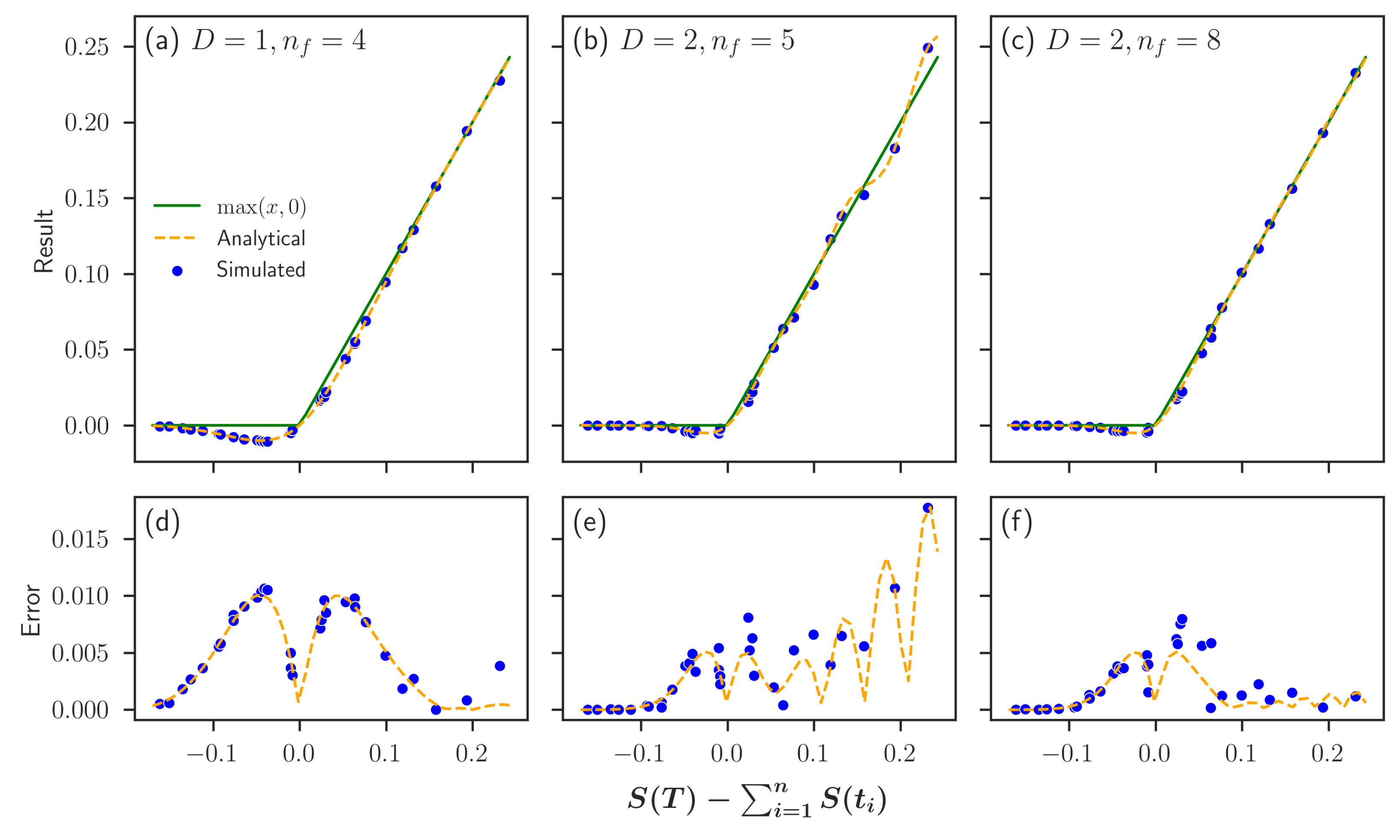
To begin with, we set our state register in each of its computational basis states corresponding to a single path taken to see the approximation for the corresponding option value. In the upper row of Figure 5, the analytical probability as well as the circuit result for shots are shown for . In the lower row, the corresponding errors are visualized. One circuit shot refers to one execution of the quantum circuit resulting in a single measurement. Observe that for approximation level of the positive part presented in Figure 5d, the error is comparatively large about 0, but it vanishes for outer values. As most evaluated values are about 0, decreasing the error about 0 is crucial. As expected, the error decreases significantly for approximation level . Nevertheless, the better approximation of the positive part also introduces the need for more terms in the Fourier expansion, the influence of which can be seen when comparing Figure 5e,f.
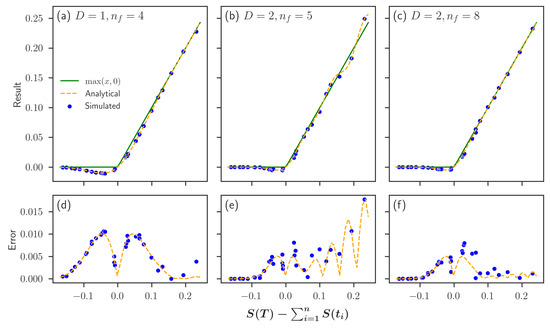
Figure 5.
Comparison of different approximation levels D and terms in the Fourier series when evaluating an Asian option on a quantum computer simulator for different paths of the underlying valuation tree. In (a–c), we compare the circuit result (blue) for executions to the analytical value (orange) we expect, and we try to approximate the option payoff (green). In (d–f), we present the respective absolute errors of the circuit and analytical results to the option payoff.
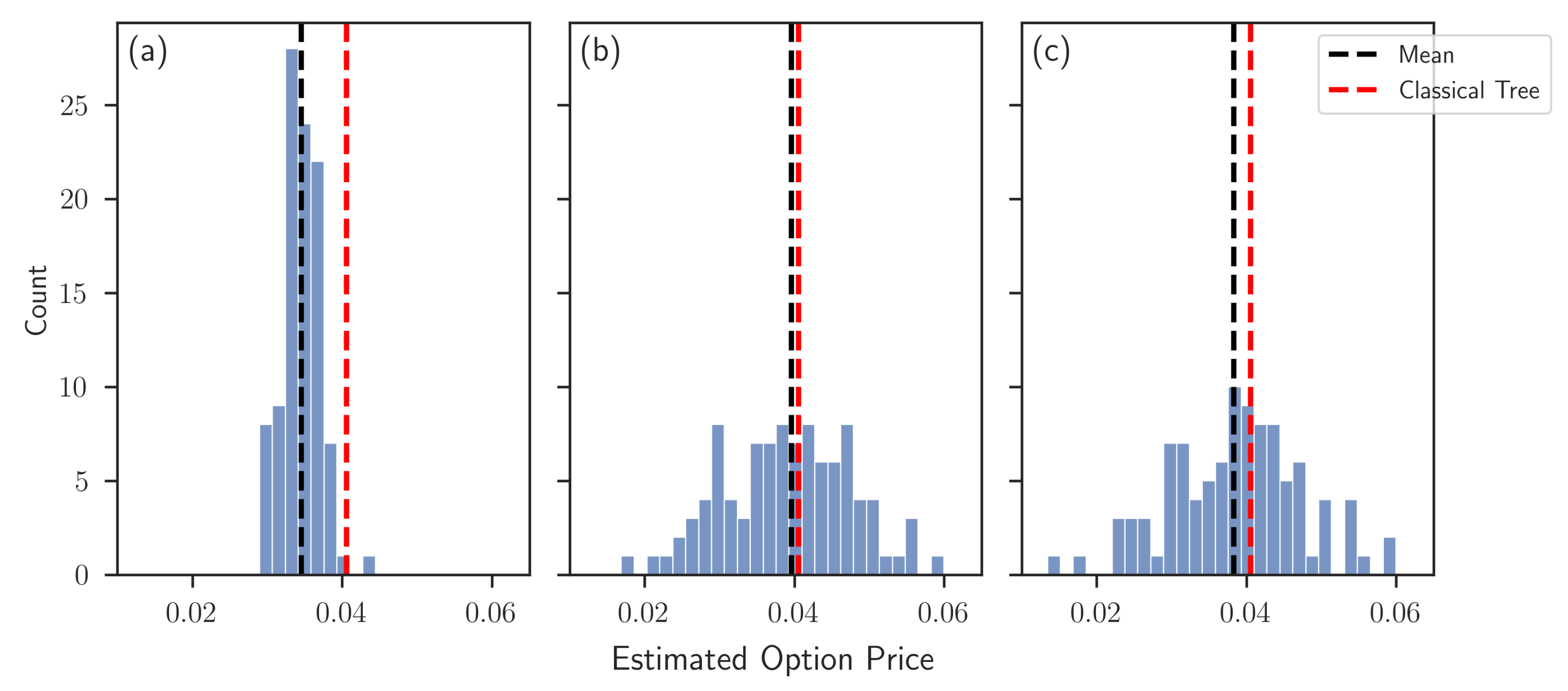
Subsequently, the state register is set to an equal superposition using Hadamard gates, enabling the simultaneous evaluation of each path. In Figure 6, results for the full pricing algorithm are shown for various parameter combinations. Each data point was generated by circuit shots, and each histogram consists of 100 different data points. The respective mean in black (which consequently corresponds to a quantum circuit being executed times) and the exact result of the classically evaluated binomial tree in red are depicted for each data set. Multiple observations can be made. In Figure 6a, approximation level results in a noticeable bias, cf. Figure 5a. By increasing the approximation level to in Figure 6b,c, the bias is reduced. Figure 6b uses a Fourier expansion with terms, and as a result, the under-estimation for paths with payoff about 0 is leveled by outer payoffs, cf. Figure 5b. Increasing the terms of the Fourier expansion to in Figure 6c decreases the outer errors as shown in Figure 5c. Consequently, the under-estimation for payoffs about 0 is no longer leveled, and the total bias increases again. Note that the over-estimation, hence, the smaller bias of Figure 5b, depends on the payoff range. When employing the algorithm for other valuation trees, additional under-estimations are possible.
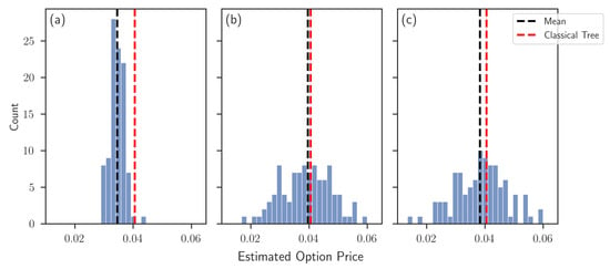
Figure 6.
Histograms of quantum simulator results for full pricing algorithm with state register in uniform superposition, i.e., simultaneous computation of all paths for time steps, gearbox approximation levels D and terms in the Fourier expansion : (a) , (b) , and (c) . 100 circuit results are presented, where each result consists of circuit executions.
In Table 1, we present the -gate count and qubit amount needed for each of the three used parameter combinations, which are currently the main criteria for a quantum circuit to be implementable on real NISQ hardware. Current state-of-the-art quantum hardware can execute circuits with reliable results with up to 30 -gate applications. Note that in our implementation, we split the main circuit into multiple subcircuits, each implementing a term for the Fourier series approximation and or , respectively. Because of this, the -gate count is the same for variants (b) and (c). The metric is dominated by the uniformly controlled rotations each requiring -gate applications as proven in Shende et al. (2006). The linear scaling in the amount of qubits needed can also be seen, increasing only in the qubits needed for the path encoding and the ancillary qubits needed for the implementation of G.

Table 1.
Required -gate counts and circuit width (number of used qubits) for a single subcircuit and number of subcircuits used in the presented algorithm with parameters (a) , (b) and (c) , for a varying number of time steps n.
6. Discussion
We developed a novel quantum circuit to efficiently price discrete floating-strike Asian options using quantum computing. The implementation uses a combination of amplitude-based arithmetics and the application of an amplitude-based unit step function to efficiently construct the fair price of the option as the amplitude of a quantum state. Additional quantum algorithms may be employed, resulting in the possibility of a quantum speed-up if larger, fault-tolerant quantum hardware becomes available in the future. This research further presents the applicability of quantum computing in the area of finance, risk management and insurance, and it should increase awareness of the upcoming changes in computational methods provided by quantum technology. The algorithm has been simulated using the Qiskit simulator by Sajid et al. (2021), showing that the expected results can be produced. The method may be generalized to use for other derivative pricing algorithms that are sensitive to discretization errors. Depending on the implementation of the valuation tree, a comparatively small amount of qubits suffices for the construction. As there are quantum computers being developed with limited qubit availability (cf. Pezzagna and Meijer 2021), this might prove to be a major advantage.
Subject to further research could be the application to different types of options such as the cliquet option (cf. Bernard and Li 2013) used for example in life insurance contracts. As they are financed by surpluses of the general account, they allow both participation at the capital market and investing the premiums rather safely in the general account. Alternatively, the employment of different quantum circuits for the more optimized implementation of the various functions is of interest. A different application of our technique would be the combination of the presented approach of using an amplitude-based positive part with established quantum algorithms utilizing a bit-based encoding. This could reduce circuit depth and qubit amounts, bringing us one step further to quantum advantage.
Author Contributions
Conceptualization, M.-O.W.; methodology, M.-O.W. and J.K.; validation, M.-O.W.; formal analysis, M.-O.W. and R.H.; data curation, M.-O.W. and J.K.; writing, M.-O.W. and R.H. and J.K.; visualization, M.-O.W. All authors have read and agreed to the published version of the manuscript.
Funding
This work was supported by the project AnQuC-3 of the Competence Center Quantum Computing Rhineland-Palatinate (Germany).
Data Availability Statement
The Python code used for data generation is available upon request.
Acknowledgments
We would like to thank Ralf Korn for general advice and constructive discussions regarding financial mathematics. We further acknowledge Luminita Mihaila for fruitful discussions on quantum computing.
Conflicts of Interest
The authors declare no conflict of interest.
References
- Bernard, Carole, and Wenbo V. Li. 2013. Pricing and hedging of cliquet options and locally capped contracts. SIAM Journal on Financial Mathematics 4: 353–71. [Google Scholar] [CrossRef]
- Blank, Carsten, Daniel K. Park, and Francesco Petruccione. 2021. Quantum-enhanced analysis of discrete stochastic processes. NPJ Quantum Information 7: 1–9. [Google Scholar] [CrossRef]
- Brassard, Gilles, Peter Hoyer, Michele Mosca, and Alain Tapp. 2000. Quantum amplitude amplification and estimation. AMS Contemporary Mathematics Series 305: 53–68. [Google Scholar] [CrossRef]
- Chakrabarti, Shouvanik, Rajiv Krishnakumar, Guglielmo Mazzola, Nikitas Stamatopoulos, Stefan Woerner, and William J. Zeng. 2021. A Threshold for Quantum Advantage in Derivative Pricing. Quantum 5: 463. [Google Scholar] [CrossRef]
- Cox, John C., Stephen A. Ross, and Mark Rubinstein. 1979. Option pricing: A simplified approach. Journal of Financial Economics 7: 229–63. [Google Scholar] [CrossRef]
- Egger, Daniel J., Jakub Mareček, and Stefan Woerner. 2021. Warm-starting quantum optimization. Quantum 5: 479. [Google Scholar] [CrossRef]
- Grover, Lov, and Terry Rudolph. 2002. Creating Superpositions that Correspond to Efficiently Integrable Probability Distributions. Available online: https://arxiv.org/abs/quant-ph/0208112 (accessed on 13 November 2022).
- Holmes, Adam, and Anne Y. Matsuura. 2020. Efficient quantum circuits for accurate state preparation of smooth, differentiable functions. Paper presented at the 2020 IEEE International Conference on Quantum Computing and Engineering (QCE), Denver, CO, USA, October 12–16; pp. 169–79. [Google Scholar] [CrossRef]
- Koppe, Jonas, and Mark-Oliver Wolf. 2022. An amplitude-based implementation of the unit step function on a quantum computer. arXiv arXiv:2206.03053. [Google Scholar] [CrossRef]
- Korn, Ralf, Elke Korn, and Gerald Kroisandt. 2010. Monte Carlo Methods and Models in Finance and Insurance. Boca Raton: CRC Press. [Google Scholar]
- Kubo, Kenji, Koichi Miyamoto, Kosuke Mitarai, and Keisuke Fujii. 2022. Pricing multi-asset derivatives by variational quantum algorithms. arXiv arXiv:2207.01277. [Google Scholar]
- Martin, Ana, Bruno Candelas, Ángel Rodríguez-Rozas, José D. Martín-Guerrero, Xi Chen, Lucas Lamata, Román Orús, Enrique Solano, and Mikel Sanz. 2021. Toward pricing financial derivatives with an ibm quantum computer. Physical Review Research 3: 013167. [Google Scholar] [CrossRef]
- Miyamoto, Koichi, and Kenji Kubo. 2021. Pricing multi-asset derivatives by finite difference method on a quantum computer. arXiv arXiv:2109.12896. [Google Scholar] [CrossRef]
- Montanaro, Ashley. 2015. Quantum speedup of monte carlo methods. Proceedings of the Royal Society A: Mathematical, Physical and Engineering Science 471: 20150301. [Google Scholar] [CrossRef] [PubMed]
- Möttönen, Mikko, Juha J. Vartiainen, Ville Bergholm, and Martti M. Salomaa. 2004. Quantum circuits for general multiqubit gates. Physical Review Letters 93: 130502. [Google Scholar] [CrossRef] [PubMed]
- Pezzagna, Sébastien, and Jan Meijer. 2021. Quantum computer based on color centers in diamond. Applied Physics Reviews 8: 011308. [Google Scholar] [CrossRef]
- Plesch, Martin, and Časlav Brukner. 2011. Quantum-state preparation with universal gate decompositions. Physical Review A 83: 032302. [Google Scholar] [CrossRef]
- Preskill, John. 2018. Quantum Computing in the NISQ era and beyond. Quantum 2: 79. [Google Scholar] [CrossRef]
- Rebentrost, Patrick, Brajesh Gupt, and Thomas R. Bromley. 2018. Quantum computational finance: Monte Carlo pricing of financial derivatives. Physical Review A 98: 022321. [Google Scholar] [CrossRef]
- Rendleman, Richard J., and Brit J. Bartter. 1979. Two-state option pricing. The Journal of Finance 34: 1093–110. [Google Scholar] [CrossRef]
- Sajid, Anis, Abby Mitchell, Héctor Abraham, AduOffei, Rochisha Agarwal, Gabriele Agliardi, Merav Aharoni, Vishnu Ajith, and Ismail Yunus Akhalwaya. 2021. Qiskit: An open-source framework for quantum computing. [Google Scholar] [CrossRef]
- Shende, Vivek V., Stephen S. Bullock, and Igor L. Markov. 2006. Synthesis of quantum-logic circuits. IEEE Transactions on Computer-Aided Design of Integrated Circuits and Systems 25: 1000–10. [Google Scholar] [CrossRef]
- Stamatopoulos, Nikitas, Daniel J. Egger, Yue Sun, Christa Zoufal, Raban Iten, Ning Shen, and Stefan Woerner. 2020. Option pricing using quantum computers. Quantum 4: 291. [Google Scholar] [CrossRef]
- Stamatopoulos, Nikitas, Guglielmo Mazzola, Stefan Woerner, and William J. Zeng. 2022. Towards quantum advantage in financial market risk using quantum gradient algorithms. Quantum 6: 770. [Google Scholar] [CrossRef]
- Vazquez, Almudena Carrera, and Stefan Woerner. 2021. Efficient state preparation for quantum amplitude estimation. Physical Review Applied 15: 034027. [Google Scholar] [CrossRef]
- Woerner, Stefan, and Daniel J. Egger. 2019. Quantum risk analysis. NPJ Quantum Information 5: 15. [Google Scholar] [CrossRef]
- Zhang, Xiao-Ming, Man-Hong Yung, and Xiao Yuan. 2021. Low-depth quantum state preparation. Physical Review Research 3: 043200. [Google Scholar] [CrossRef]
- Zoufal, Christa, Aurélien Lucchi, and Stefan Woerner. 2019. Quantum generative adversarial networks for learning and loading random distributions. NPJ Quantum Information 5: 103. [Google Scholar] [CrossRef]
Publisher’s Note: MDPI stays neutral with regard to jurisdictional claims in published maps and institutional affiliations. |
© 2022 by the authors. Licensee MDPI, Basel, Switzerland. This article is an open access article distributed under the terms and conditions of the Creative Commons Attribution (CC BY) license (https://creativecommons.org/licenses/by/4.0/).

