Inhomogeneous Financial Markets in a Low Interest Rate Environment—A Cluster Analysis of Eurozone Economies

Abstract

In the present paper, we investigate the financial homogeneity of the euro area economies by contrasting eurozone countries’ responses to monetary policy steps to the theoretical assumptions of the liquidity trap phenomenon. Our assumption is that the euro area economies are not completely homogeneous. Hence, in a zero-interest rate environment, the asset holding decisions of economic agents exhibit detectable differences across countries. We verify our assumptions using Eurostat data. We use the financial asset stocks of the euro area countries to cluster the countries concerned. Previous literature has not examined changes in the ratio of financial assets to GDP, nor differences in structural changes in the total stock of financial assets under the zero lower bound. The paper uses k-centers cluster analysis based on Euclidean distance for detecting changes in the portfolio holdings of eurozone economic actors owing to economic crises and monetary policy responses. The results confirm that euro area financial markets are fragmented. There are significant differences across asset markets of different Eurozone countries, both during and after the crisis. Despite some similarities in the portfolio rearrangement across countries, the ECB’s monetary policy does not have a uniform impact on euro area financial markets, and notable differences prevail in the financial asset structures of the economies concerned.

1. Introduction

Keynes integrated monetary theory into general economic theory. He broke with the dichotomous approach of classical and neoclassical economists. He examined the effectiveness of monetary policy and the limits of monetary policy. In light of his liquidity preference theory, he assumed that below a certain level of interest rates, monetary policy becomes ineffective because of the portfolio choices of economic agents. Today, economists unanimously refer to this phenomenon as the liquidity trap. A liquidity trap occurs when the market interest rate falls to a low level. This diverts economic agents’ intentions away from other elements of wealth holding and towards money holding (Keynes 1936).

Keynes based his theory of the liquidity trap on the empirical phenomenon that, despite moderate interest rates in the 1930s, the economy failed to recover and investment activity failed to pick up. He sought solutions to the problems of the British economy in the 1930s and made economic policy recommendations. The ineffectiveness of monetary policy in achieving near-zero interest rates was, for several decades, to become the subject of a rather theoretical debate.

Its practical economic policy relevance came about in the context of the stagnation of the Japanese economy since the early 1990s and the monetary responses to support growth. The theoretical debate also flared up again (Werner 2005; Tatay and Tatay 2020). In Japan, an increase in the money supply did not even induce the proportional increase in prices assumed under monetary neutrality, besides being ineffective on real economic performance (Krugman et al. 1998; Itoh and Shimoi 2000; Ueda 2001).

Bibow (2013) argues that liquidity preference theory is misunderstood and underemphasized by many. Bibow cites Keynes’ liquidity preference theory as a highly relevant theory. He also saw it as a way to assess the phenomena of the 2008 global financial crisis (Lhuissier et al. 2020).

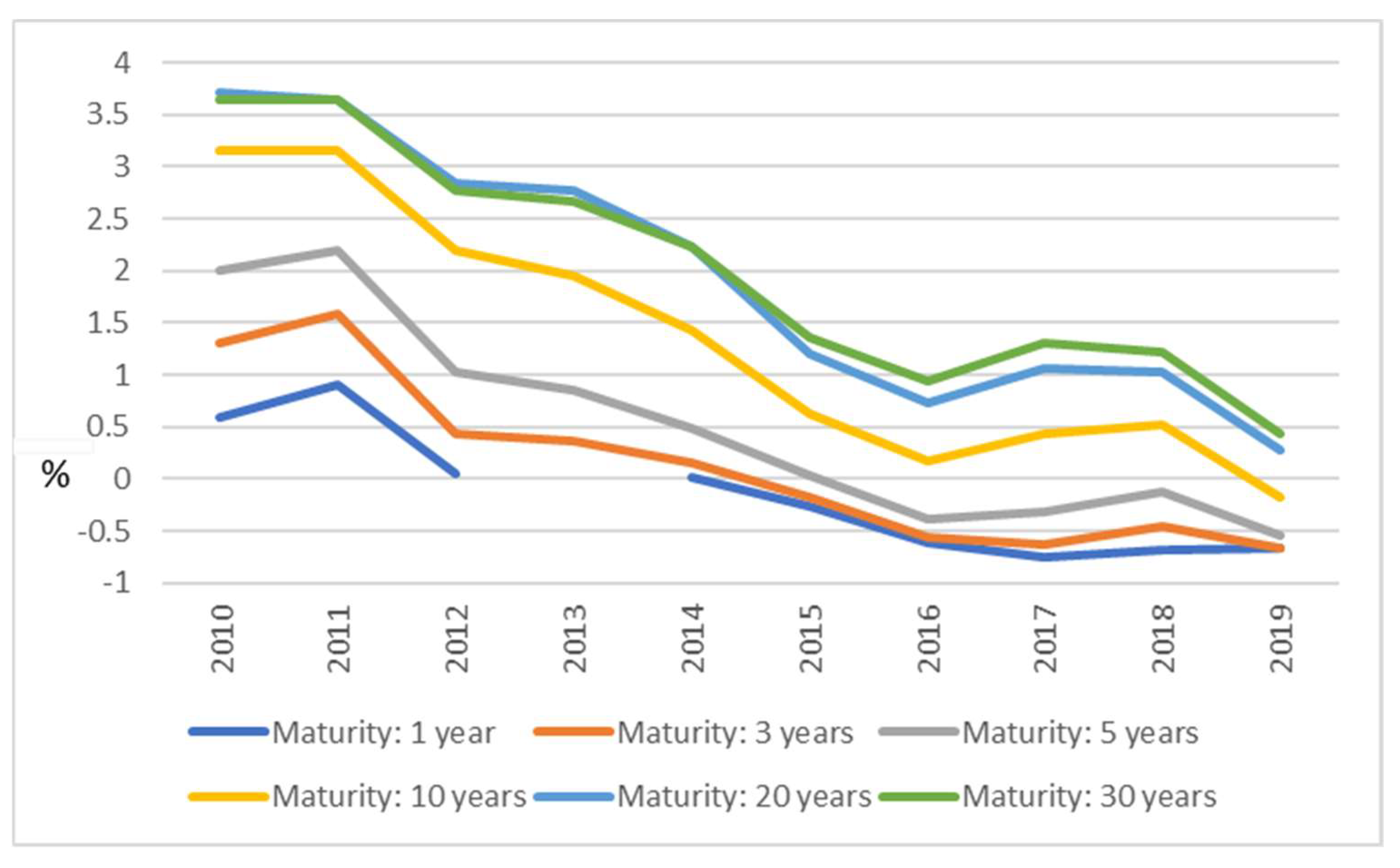
As a consequence of the global financial crisis, the European Central Bank also started to cut interest rates after 2010. In 2014, it launched its QE program, bringing the entire euro yield curve under control (Kuroda 2016; Kiley 2018). Figure 1 shows the euro spot rate yield curves over the period 2010–2019.

Previously, the phenomenon of a zero-interest rate environment was assessed within a single country’s economy. By 2010, the euro area was made up of 16 countries, with three more soon to join soon (the three countries joining after 2010 can almost be considered members by 2010, as they had to meet the strict criteria for membership several years before joining). Monetary policy actions by the European Central Bank should have the same effect in each economy. The ECB’s interest rate moves should entail a reallocation of similar financial wealth among economic agents in the euro area economies. Under Keynes’ liquidity preference theory, in a zero-interest rate environment, this reallocation is not only of a similar nature, but is also assumed to be of a marked magnitude. In the present paper, we aim to investigate the financial homogeneity of the euro area economies by means of the theoretical assumptions of the liquidity trap phenomenon.

Our assumption was that the euro area economies are not completely homogeneous. Hence, in a zero-interest rate environment, the asset holding decisions of economic agents would exhibit detectable differences across countries. We assumed that the differences due to these divergences persisted even when the ECB controlled not only short, but also long-term, yields.

We intended to verify our assumptions using Eurostat data. We used the financial asset stocks of the euro area countries to cluster the countries concerned. The homogeneity or heterogeneity, and the changes in clusters, would confirm or refute our hypothesis that the zero lower bound and quantitative easing measures affected the portfolio decisions of economic agents but country specific differences persisted.

Due to the financial turbulence COVID-19 caused all over in the world, the ECB continued with a zero-interest rate environment and extended its asset purchases and, as a result, avoided the return of extremely high yields that characterized the sovereign debt crisis (Havlik et al. 2022). With the outbreak of the Russian–Ukrainian conflict, the ECB did not change its monetary policy stance and maintained the ZLB (zero lower bound) until July 2022 in contrast to other major central banks, like the Fed and the BoE. The analysis intentionally does not cover the period after 2020 because the economies were then hit by both a negative supply and demand shock and, from 2022, an unprecedented inflationary period followed in the Eurozone and the world which is not to be explained by the liquidity trap phenomenon.

Our results should also be placed in an international context, in a period with strongly deviating monetary policies. From 2010 to the end of 2015 the Fed eventually maintained the effective zero lower bound, while the ECB was gradually cutting its policy rate to zero (apart from two minor rises in 2011) by March 2016 and keeping it at the same level until the end of the period examined in this study. The Fed kept on tightening monetary policy until March 2020 and started its tapering program at the end of 2013, while a higher volume QE was only launched at the end of 2015 by the ECB. The BoE started its first raise in the base rate at the end of 2017, which was continued by further increases, while the Bank of Japan maintained a below zero level of policy rates from the beginning of 2016. Apart from adversely affecting the yield curve, these dissimilar monetary policy actions could also influence the choice of domestic actors between domestic and foreign assets, which the present paper does not separate within the various asset classes, due to limitations in size and scope.

The structure of the paper is as follows. First, we review the literature. In this section we discuss the main elements of Keynes’ liquidity preference theory, and the emergence of the liquidity trap. We then turn to the literature on the fragmentation of the euro area. In the materials and methods section, we present the empirical data of the study and describe the cluster analysis method used. In the subsequent results and discussion section, the results obtained by applying the k-centers cluster method are presented and evaluated. In the final conclusions section, a summary evaluation of the results obtained is made, and the applicability of the results and directions for further research are indicated.

2. Literature Review

2.1. Liquidity Preference and the Liquidity Trap Phenomenon

Monetary theory was integrated into general economic theory by Keynes. He broke with the dichotomous approach of classical and neoclassical economists. The main pillar of monetizing economic theory lies in the introduction of the liquidity function. Keynes wanted to circumscribe how a sufficient amount of capital could stream to finance investment, and, as a consequence, he dealt with the factors affecting the wealth holdings of economic actors. He examined how interest rates regulated by monetary policy influence the portfolio decisions of economic actors. This directed attention to the occurrence of situations in which monetary policy could become ineffective. This situation is regarded as the “liquidity trap”.

Though the term, “liquidity trap” is attributed to Keynes by many, thanks are, indeed, to be rendered to Robertson (Hicks 1942; Barens 2018). Robertson (1940) referred to this phenomenon in his work ‘Essays in Monetary Theory’ as ”liquidity trap for savings”, that is savings are absorbed in financial assets and do not finance investment activity, so, in contrast to Keynes and his followers, Robertson disapproved of the lack of liquidity instead of its abundance. Today economists uniformly consider a situation a liquidity trap when, as a consequence of the excessive liquidity, interest rates bump into a lower bound and deflationary expectations constrain the room for maneuver of monetary policy (Caballero and Farhi 2018; Cook and Devereux 2011; Horváth and Szini 2015).

As the liquidity trap issue is traced back to the theoretical considerations of Keynes, we, therefore, first survey the views of Keynes on money holding and factors forming interest rates on the basis of his book ‘The General Theory of Employment, Interest and Money’ (Keynes 1936). In this book, Keynes emphasized questions affecting interest rates, or what the impact of the evolution of interest rates would exercise on the economy. While neoclassical economists conceived interest rate as a factor equating savings and investment, Keynes took a sheerly different standpoint. As a result, he approached the components determining interest rates in a different way compared to economists preceding him. He represented a different viewpoint on what effects the magnitude and change of interest rates exert on the economy.

Keynes defined savings as the part of income that is not used for consumption for a given period of time. Propensity to save is, thus, influenced by propensity to consume in his opinion. The wealth saved needs to be held in some form or another, and the saving decision should be followed by an investment decision. Nobody can save without purchasing property or assets. In our study the structure of wealth is the focus. Assets can consist of money, loans or capital goods. At the macro level most individuals are under constraints. Though individuals can choose what amount of money to hold within their overall portfolio, as a whole, they are bound to own the amount of money created by the banking system (Brady 2018).

The individual, thus, makes the decision on what proportion of income should be spent on consumption or saving. After this, he or she should choose the form of holding wealth stemming from current income saved and earlier savings. Keynes stressed that this decision is much affected by the individual’s need for liquidity. The structure of wealth holding depends on the extent the individual is willing to waive the opportunity to keep his wealth in assets which can at any time be converted into other property or assets to be spent. The liquidity needs of the individual can be described by a function which shows what proportion of wealth the individual desires to hold in the form of money under given circumstances. Interest is the reward for giving up liquidity. As a consequence, the interest rate is the rate of the price individuals expect in exchange for giving up hoarding money.

The interest rate does not, in reality, establish a balance for the volume of investment with the propensity to save (Backhouse 2020). The interest rate equilibrates the need for holding cash and the amount of money available. Keynes alluded to the demand for liquidity as a factor exercising a potential tendency to the money hoarding desires of the totality of the actors of the economy. At a lower interest rate, the totality of individuals would like to hold more cash than is available. At too high an interest rate, an amount of money would arise that individuals would not desire to preserve. This leads to the conclusion that beyond the individuals’ demand for liquidity the amount of money is the other factor affecting interest rates. Keynes considered the amount of money as given, as exogenous for the totality of individuals. The amount of money depends on the money creation of the banking system, an external condition.

On the whole, Keynes regarded the evolution of interest rates as important, as these played a decisive role in the realization of investment in his assessment. Interest rate is the reward for giving up money, or liquidity. Interest rates are affected by speculative money demand and the available amount of money. Speculative demand for money is influenced by the interest expectations of individuals. Interest rates evolving in the market can reach a lower value at which the actors of the economy reckon on a rise in interest rates by all means, and, therefore, the interest rate elasticity of the speculative demand for money becomes infinite. Keynes was proposing a lower limit as such, at some 2–2.5%. Later, economic thinkers defined the term liquidity trap starting out from this conception.

The liquidity trap actually became a well-known economic principle among economists with the graphical illustration of Hicks, especially through the use of IS-LM curves. Below a certain interest rate level, the demand for money is perfectly elastic, monetary policy intervention is ineffective as concerns output, and is not able to stimulate economic performance (Hicks 1937, 1974). Hicks conjectured that short-term interest rates cannot take negative values permanently, while long-term ones are supplemented with liquidity premia. Furthermore, he objected to the approach of Keynes in that present interest rates depend on their own future expectations. In Hicks’ view, this only holds for long-term interest rates, as they depend on the expectations for future short-term rates, but not for short-term interest rates, as the latter are defined by the present demand and supply of money free of transaction costs, in contrast to any type of security, the purchase of which is cumbersome. The substitution chain formed by money and securities justifies the various rates of assets with different maturities, the various interest rates of money, which allow compensation for the risk of capital loss.

Following on from Hicks it became common knowledge that the lower bound practically prevents exercising control over money supply in the case of falling prices (Boianovsky 2004).

According to Patinkin (1974), in the original wording of Keynes, it is by all means true that the greater the interest elasticity of money demand, the greater the monetary expansion needed for the restoration of equilibrium, and, what is more, above a certain point, monetary policy might become completely ineffective. Nevertheless, he argues that Keynes only theoretically presumed a situation in which monetary policy becomes ineffective.

With the help of elasticity calculations, the monetarists Brunner and Meltzer (1968) proved that such a liquidity trap does not exist in an absolute sense, and only “asymptotic traps” can occur, in which the effectiveness of monetary policy variables converge to zero. In their view, the liquidity trap phenomenon should be separated according to the various effects of monetary policy on money supply, interest rate levels, bank lending and money demand. They introduced a separate term, named “basis trap”, for the case in which the central bank unsuccessfully attempts to affect the above variables with the help of increasing M0.

Later Meltzer (1999), referring to his common study with Brunner, published in 1968, highlighted that the positive impact of money supply expansion on the price of securities should also be taken into consideration. The relationship between money supply and wealth should not be ignored, especially in cases when individual financial assets, among foreign and domestic, as emphasized by McCallum (2000), or capital goods and bonds, pointed out by Tobin (1947, 1971), are not perfect substitutes. This wealth effect is excluded from IS-LM analyses. He came to the conclusion that monetary policy can remain effective independent of the interest rate reaching the lower bound, as the central bank can freely purchase and sell securities, which are not perfect substitutes for money and bear non-zero interest rates (Kahn 1972; Cardim de Carvalho 2010; Runde 1994).

In sum, the liquidity preference theory of Keynes can be found in the economic literature as a benchmark in many discussions. Though the relationship between the change in interest rates and the portfolio decisions of economic actors has been explained from many viewpoints, the relationship itself has been treated as evidence (Novák and Tatay 2021a).

2.2. The Fragmented Nature of Eurozone Economies from the Point of View of Monetary Regulation

According to Horvath (2018), the fragmentation of eurozone financial markets increased after the 2008 global financial crisis. Risk premia meant bank interest rates reacted to the interest rate decisions of the ECB to a lesser extent. As a consequence, the effectiveness of monetary policy deteriorated. As a result of the differing country risk assessment of the particular eurozone countries, the ECB rate cuts did not appear in each country’s bank rates (Lucotte 2015). The situation improved after 2012; though, the problem further prevailed. In his view, the application of unconventional monetary policy instruments has contributed to the reduction of fragmentation.

Agba et al. (2022) also examined whether the reaction to ECB monetary policy steps was perceivably different in the various eurozone economies. Within the particular countries, indicators of more industries were subject to analysis in comparison to the aggregated indicators of the same economies. The indicators used encompassed bank profitability, countries’ indebtedness etc. As a final conclusion of these examinations, they also ascertained that the industry level responses to ECB operations were different in the particular eurozone economies. That is, the various economies reacted in a non-homogeneous manner to monetary policy measures. The fragmented nature of the banking system of the eurozone was the starting point for analysis of in 2015, investigating the realization of ECB monetary policy. In his view, the banks of the periphery economies detached from the integrated eurozone interbank market after the 2008 global financial crisis. This could be primarily traced back to the sovereign debt crisis, or to the unfavorable macroeconomic data of the particular economies. Banks of the periphery economies were mostly indebted to the banks of core economies. For the repayment of debts, they had to apply to the ECB for supplementary funding, as if they had required central bank loans for their own lending activity. The liquidity withdrawn this way appeared in the banks of countries in the center as well. Due to this duality, the interest rate policy of the ECB could not influence eurozone economies in a uniform way. Vari (2015) justified these assumptions empirically.

The uniformity of eurozone financial markets was examined by Karadima and Louri (2020) by analyzing bank competition and bank credit risk among eurozone (EU19) economies and between center and periphery economies in the period between 2005 and 2017. Their investigations underpinned that there were perceivable differences in the particular countries’ banking markets in respect of competition and lending. Significant deviations existed between the center and the periphery. These differences became even stronger after the 2008 financial crisis.

The research conducted by Gori (2018); Andreeva and García-Posada (2021); Ijtsma et al. (2017) corroborated the fragmented nature of eurozone banking markets. This fragmentation further strengthened after the 2008 crisis. The various banks decreased the diversification of their assets in the international markets within the eurozone as well. This process aggravated the disintegrated nature of interbank markets.

2.3. The Fragmented Nature of Eurozone Economies from the Point of View of Fiscal Policy

In the euro area, monetary policy is conducted by a central body under the ECB. However, the conduct of fiscal policy was kept under the responsibility of national governments. Different fiscal policy actions can affect the conduct of monetary policy. Several studies point to this.

A study by Sargent (1999) directly showed that fiscal policy could severely constrain the scope for monetary policy. According to the study, the debt of the state might be so large that it requires monetization. Thus, although monetary policy is legally independent, its operations are influenced by fiscal policy.

The links between public finances and the financial sector in Western economies were highlighted by Acharya et al. (2012). The problems of fiscal overstretch in Almaty affect the financial sector on the one hand and impact the non-financial sector on the other. The undercapitalization of the financial sector after the 2008 crisis required recapitalization. However, recapitalization by the state put a strain on public budgets. The increase in sovereign debt increased the risk of sovereign debt. The increased financing needs of general government worsened the financing possibilities of non-financial sector companies. Expected tax increases worsened growth prospects. The increasing burden on public finances was seen to affect the economy through several channels. The state of public finances affected the functioning of the banking system.

He and Krishnamurthy (2013) studied the dynamics of risk premia during crises. The areas of study were asset markets, where the marginal investor is a financial intermediary. Markets can be supported by the state from several sides. This can reduce the cost of borrowing for intermediaries. It can help to avoid undercapitalization through capital infusion. The budget can buy risky assets.

Dantas et al. (2022) studied the relationship between bank risk and reserve requirements for state guarantees. The study shows that the rules for the provision of state guarantees changed with the creation of the euro area. State guarantees affect banks’ reserve holdings. In addition, the provision of guarantees affects tail risk. For these reasons, the impact on bank profitability can be detected.

Silva (2021) examined the relationship between fiscal deficits and banks’ aggregate credit risk. They analyzed whether the government can compensate banks for their losses. Compensation can be direct monetary infusion or the design of stabilization policies. If the budget deficit limits government intervention, it impairs the maintenance of financial stability.

Of course, the structure of the stock of euro area financial assets is also affected by changes in exchange rates. The evolution of exchange rates is influenced by the different actions of the various central banks. Dedola et al. (2021) assessed the impact of the Fed and ECB asset purchase announcements on the dollar and euro exchange rates. They found that QE operations influence exchange rates.

In our empirical analysis, we refer to euro area government debt. In our assessments, we point to interpretative frameworks that also appear in the above literature.

The above literature leads us to the conjecture that the fragmentation of eurozone financial markets is a generic phenomenon to take into account when analyzing the changing pattern of economic actors’ portfolio decisions in times of above, or close to, zero interest rates.

3. Research Gap

The liquidity preference theory offers a new semi-trend approach to explaining the financial fragmentation of euro area economies. The zero-interest rate level over the period 2010–2019 may have both amplified and mitigated the divergence. Individual economies may have reacted differently to the ECB’s monetary policy actions. Previous literature has not examined changes in the ratio of financial assets to GDP, nor differences in structural changes in the total stock of financial assets. The authors argue that examining differences across countries can be important for understanding the financial impacts of monetary policy. Our study complements the assessment of differences in financial markets across euro area economies.

4. Results and Discussion

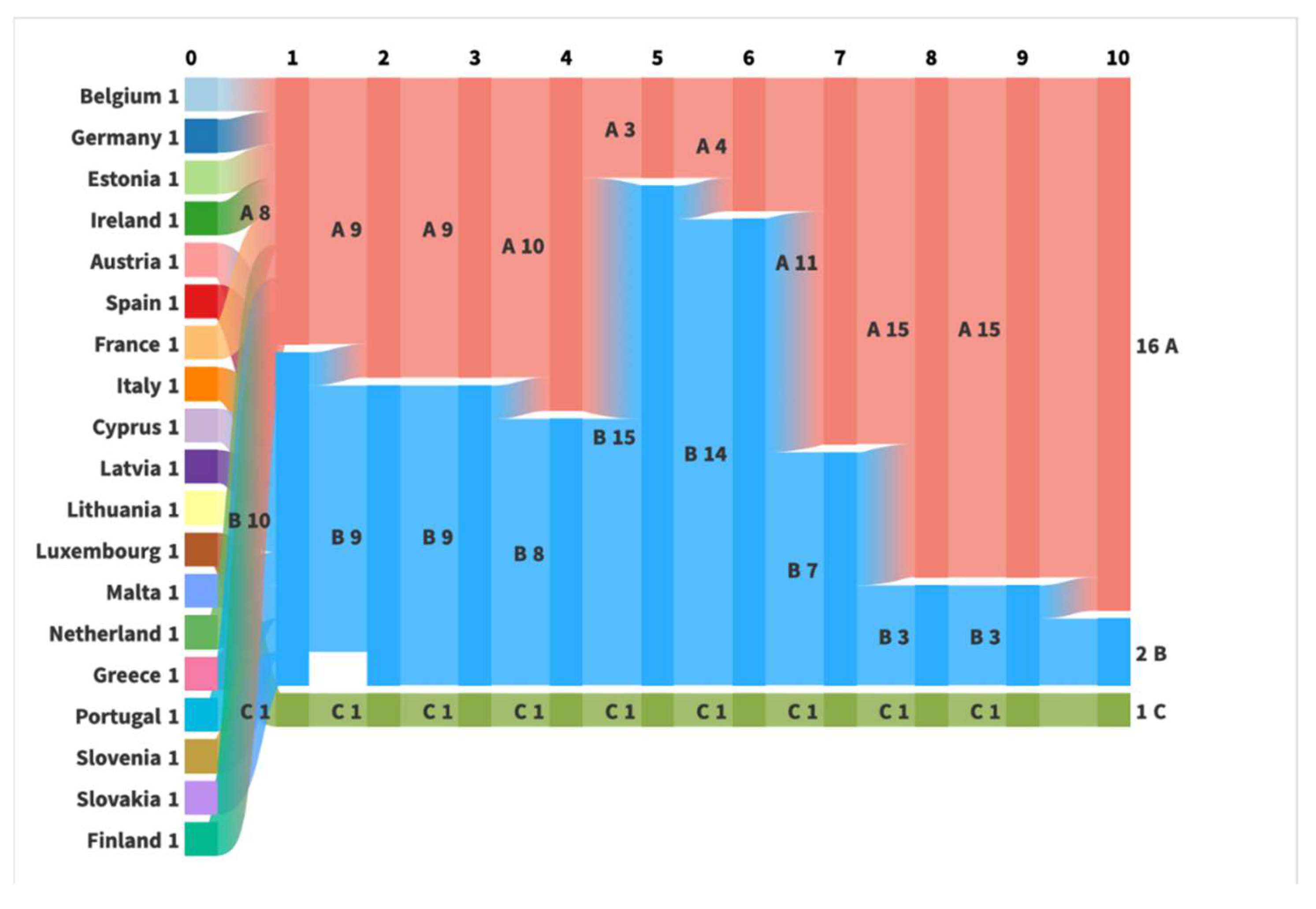
In the dynamic analysis the most obvious phenomenon was the converging behavior of the countries after the sovereign crisis in the eurozone. Whereas at the beginning more or less half of the countries belonged to the first (financially stronger) and half to the second (financially weaker) cluster, after 2013 most of the countries moved to the latter group. Furthermore, after the introduction of the effective zero lower bound and the quantitative easing measures, most of the countries managed to catch up with the first group, as concerns the financial investment structure. Luxembourg formed a third group with a very strong dominance of the first principal component. These situations are shown in Figure 2.

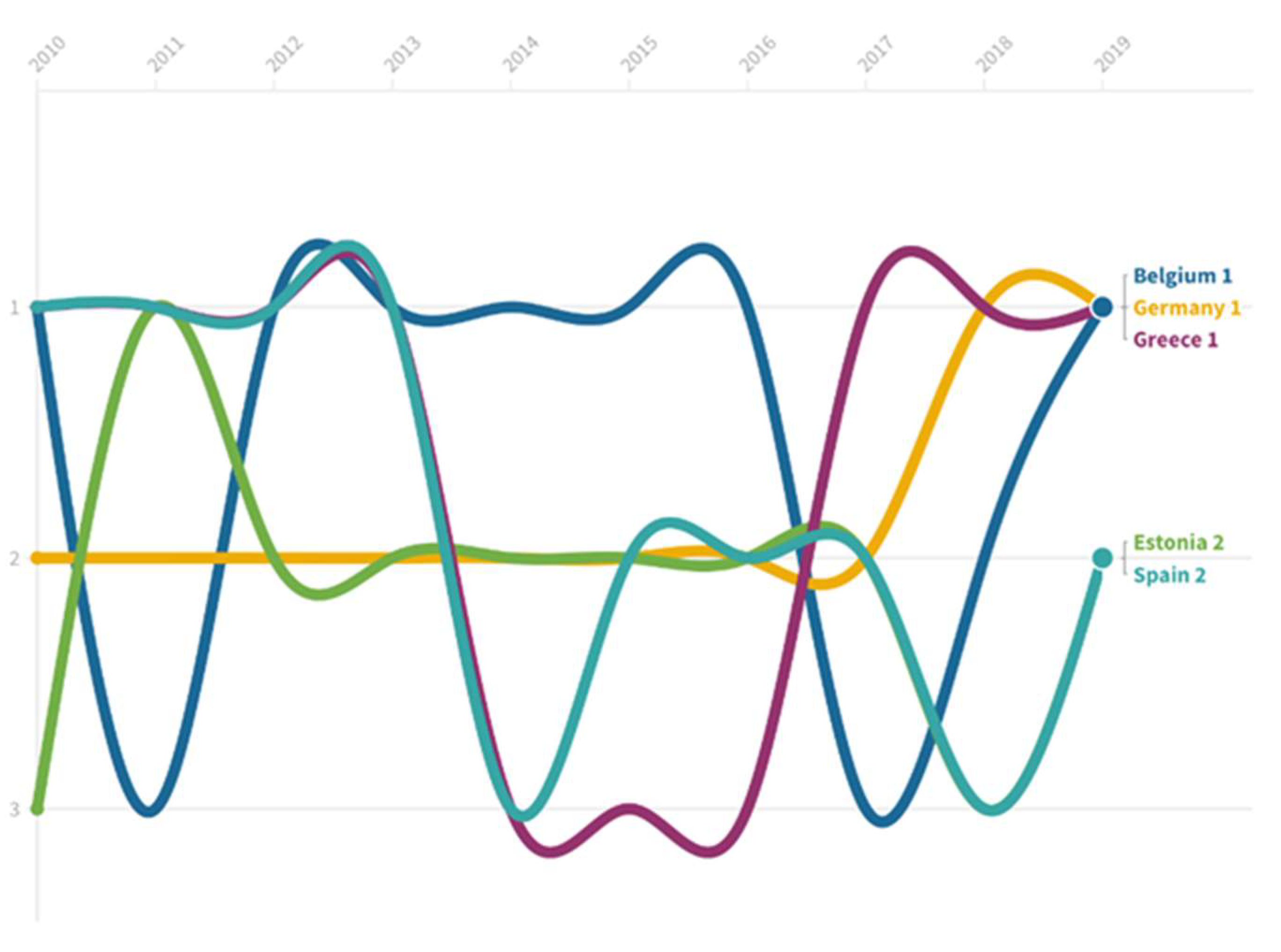
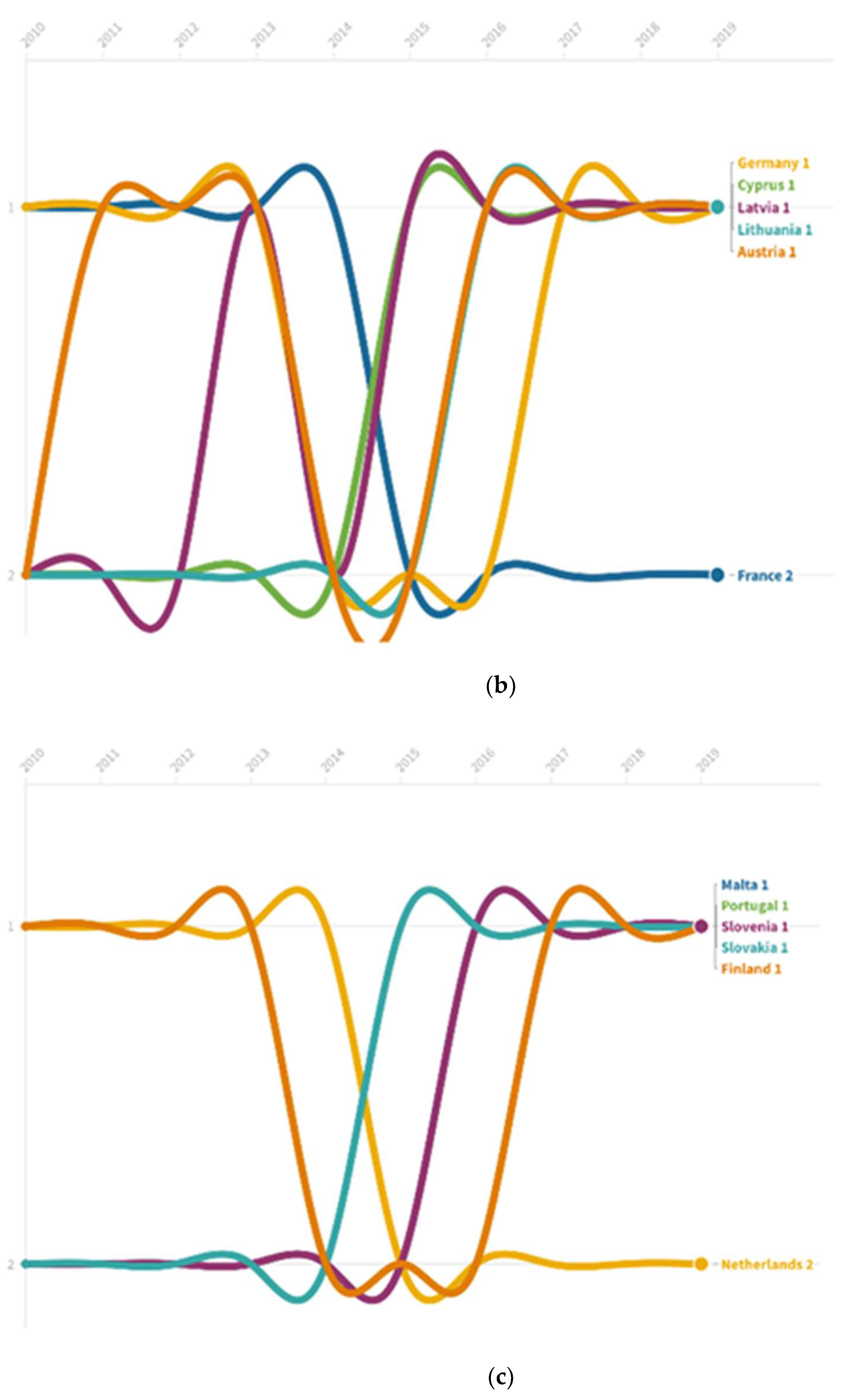
Between 2010 and 2013 countries belonging to the first cluster (A) had a somewhat below average value for the first principal component, which means less financial assets in general, higher than average for the second component, that is higher volume of other deposits or, in other words, non-transferable deposits, and lower than average for the third principal component, currency. Countries belonging to this first group were Belgium, Germany, Estonia, Ireland, France, the Netherlands, Portugal and Finland. The second group (B), consisting of the rest of the countries (Greece, Spain, Italy, Cyprus, Latvia, Lithuania, Malta, Austria, Slovenia, Slovakia), had somewhat higher levels of financial assets in general than the first cluster (less negative relationship with the first component) but much higher currency-to-GDP levels and lower savings in insurance and technical reserves. Until 2014, only Austria and Latvia changed their positions, both moving to the first group from the second, Austria in 2011 and Latvia in 2013. In this period, the most representative (closest to the cluster centroid) country in the first group was Germany, while for the second it was Italy and Spain. In 2014, a lot of countries (Belgium, Germany, Estonia, Latvia, Austria, Portugal and Finland) moved to the second group, probably due to the effects of the sovereign debt crisis on portfolio decisions. The central country in this second group remained Spain in 2014. Some rearrangements occurred also in 2015 (the Netherlands and France went to group B, while Cyprus, Latvia, Slovakia moved to group A), but the number of countries belonging to the second group remained almost the same; there was a slight reduction from 15 countries to 14 countries. Nevertheless, the most spectacular change in 2015 was that the main features of group A and B were reversed, while group A became the country group with a relatively higher proportion in financial assets than the other group, higher-than average currency holdings but lower-than-average insurance reserves, in particular, whereas group B could be described with lower savings to GDP in currency, and higher insurance technical reserves (other deposits ceased to play an important role in the formation of clusters from 2014 onwards). This change in characteristics prevailed until the end of the whole period considered. In 2015, the ECB introduced a series of monetary easing measures and, as a result, the number of countries in the second group (B) declined to 7 in 2016 and then to 3 and 2 in 2017 and 2019, respectively, which meant that both the effective lower bound and the asset purchase programs caused a strong convergence in the portfolio structure of the countries under examination if countries were only observed in a two-cluster framework (see Figure 3a–c). The most representative country for group A was Austria between 2017 and 2019 and France for group B, but for this second group the distances from the centroid were increasing over the same years.

The detailed move of countries between the two groups is reflected in Figure 3a–c.

As some countries (namely the above-mentioned Luxembourg, forming a separate cluster in every analysis) still behaved as outliers, after filtering out Luxembourg, in a three-cluster representation, as well, they were dropped one by one from the list of countries examined (first Cyprus, then Malta, Ireland and the Netherlands, respectively). With 14 countries remaining, the three clusters formed in the particular years between 2010 and 2019 were easily distinguishable, based on the three principal components. Now that the component correlations had changed, short-term debt securities, currency and investment fund shares, and transferable deposits became the most important explanatory factors for the second and third components, while the first component remained most strongly correlated to the general level of financial assets.

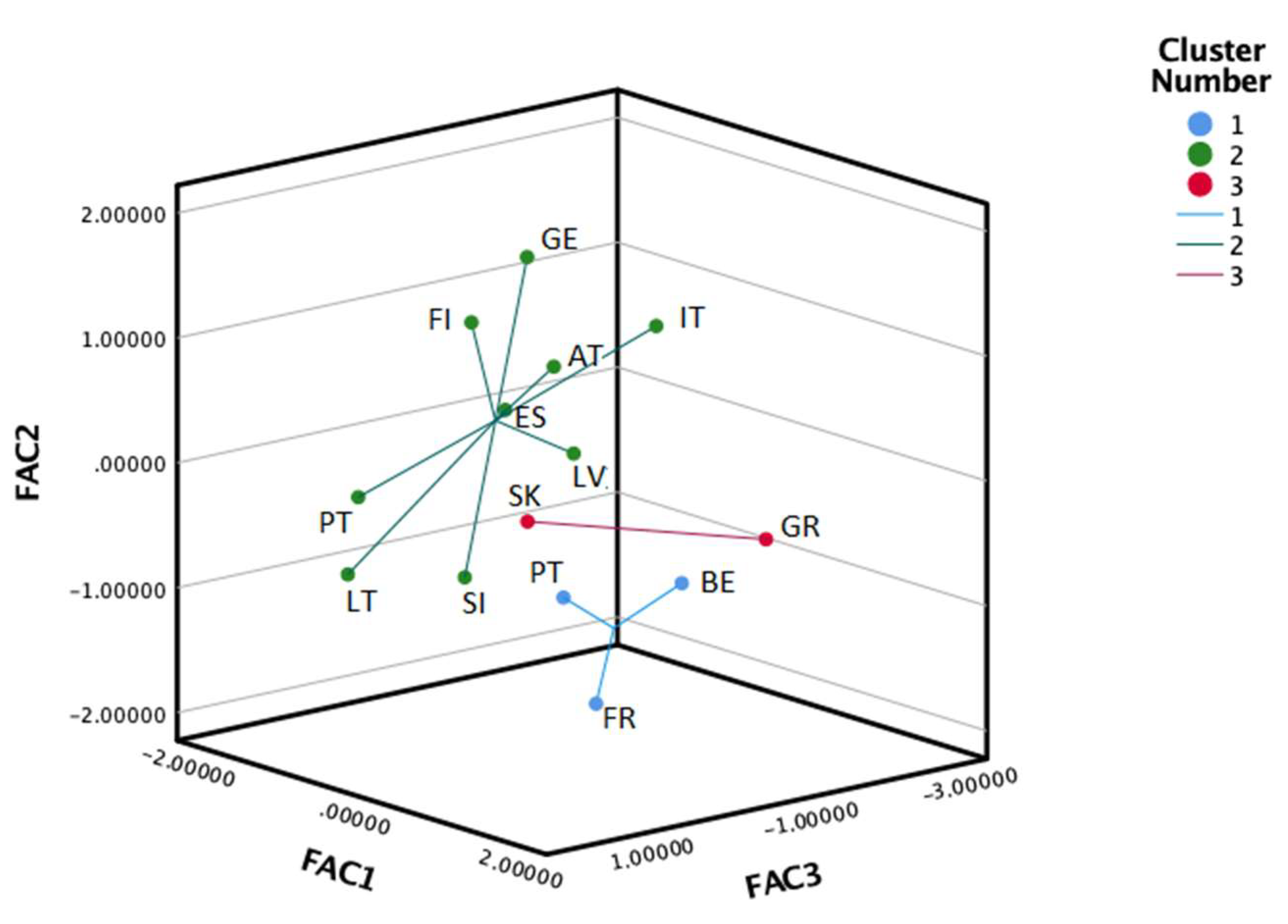
In 2010 (see Figure 4), the “truncated” sample was clearly separable for a three-cluster grouping. In the first cluster, Belgium, Greece, Spain and Portugal had higher scores for the first component (generally higher-than-average financial assets), and lower-than average values for the second and third components (less transferable deposits and short debt securities and more currency). The second group of countries (consisting of Germany, Italy, Latvia, Austria, Finland) had somewhat lower than zero factor scores for the first and second principal components, but higher loadings for the third (representing somewhat higher currency and transferable deposits and lower short-debt securities holdings). The third group of countries (including Estonia, France, Lithuania, Slovenia, Slovakia) had an outstanding score for the second component (higher short-term debt securities and lower currency holdings), while having the lowest for the first and the third components. Belgium had the highest scores for the first component (corresponding to a general level of financial assets), France for the second (highest weight of short-term debt securities and lowest of currency), and Germany for the third component (a dominant transferable deposit holding within the overall portfolio of the total economy).

In 2016 (see Figure 5), which can be regarded the first year in which the zero lower bound was in effect, most of the countries were massed in the second cluster with lowest scores for the first component and highest for the second and the third, meaning that the share of currency had a lower and transferable deposits and investment fund share, holding a higher weight in the majority of the countries, especially in countries with lower-than-average financial assets-to-GDP, in most of the financial asset categories considered. Belgium, France and Portugal formed the first cluster with most extreme data, an overall high level of financial assets-to-GDP (this time France leading the list) and lowest transferable deposit and currency holdings. The third group only covered Slovakia and Greece, countries with negative scores for all the components, low levels of financial assets, in general, high levels of transferable deposits, in particular, and high currency holdings.

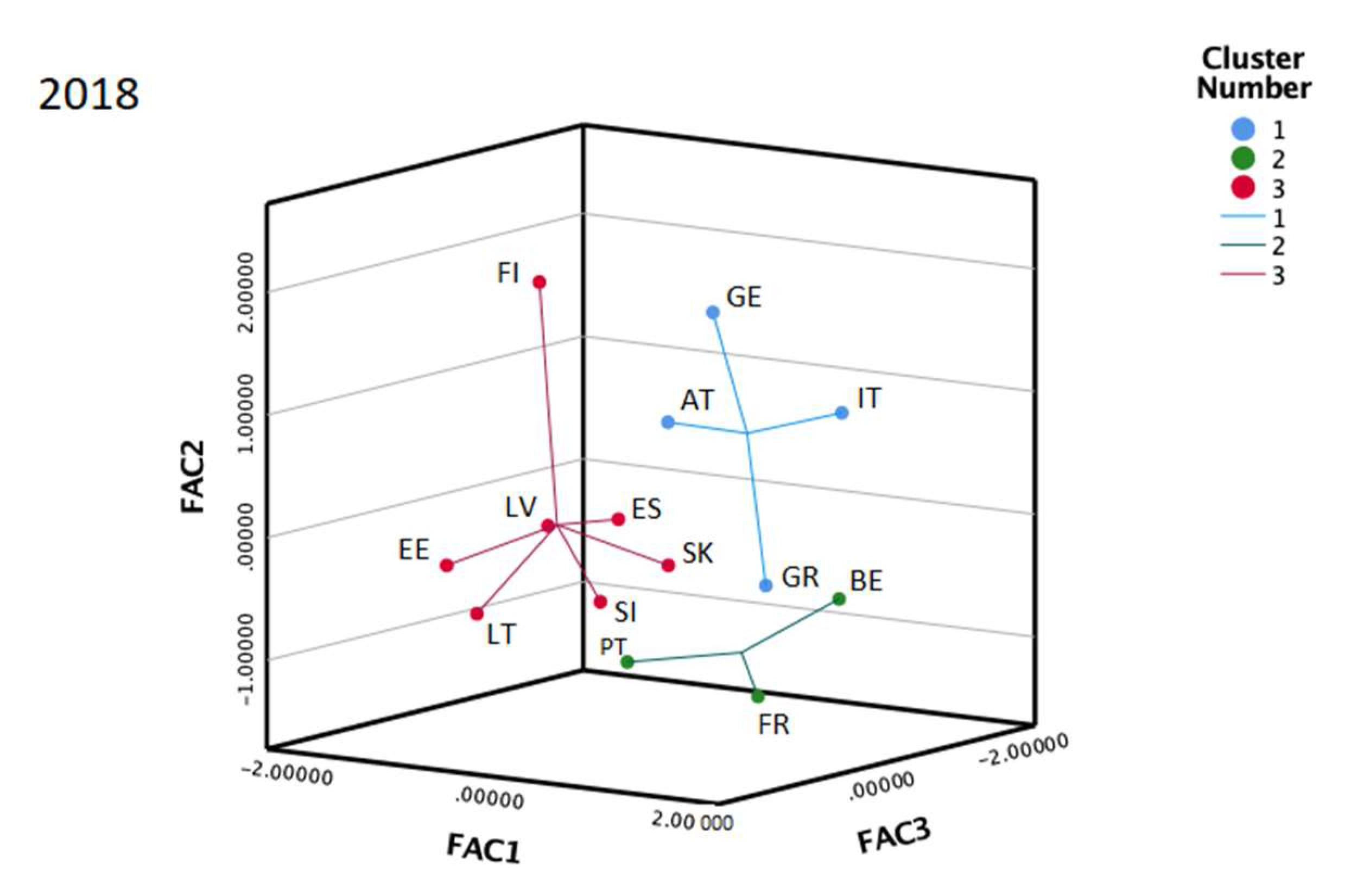
In 2019 (see Figure 6), it was still the second cluster with the greatest number of members having a low but positive score for the first component (overall level of financial assets) and a negative score for the second component (meaning this time higher-than-average currency holdings), and close to zero score for the third component (which was strongly correlated with transferable deposits and investment fund shares). The first group, with France and Portugal, having the highest level in financial assets, in general, seemed to have suffered little from low interest rates, as currency holdings remained at levels much below average and short-term debt securities above average, while the level of transferable deposits (and investment fund shares) was still below average. The third group (encompassing Estonia, Spain, Latvia, Lithuania, Finland) consisted of countries with much lower-than-average financial assets than the two other clusters, relatively low currency holdings but higher-than average savings in transferable deposits and investment fund shares.

While in 2010 more than half of the countries had a relatively high weigh of currency in their portfolio, and their number was reducing until 2016, the opposite process evolved between 2016 and 2019, with more and more countries becoming members of the “high-currency-holding” group. Among the non-interest paying instruments, transferable deposits did not become evidently more favorable among the “core” countries and short-term deposits disappeared as a cluster forming variable after 2014, to be replaced by investment fund shares after 2017. Between 2010 and 2015 Belgium was the leading country, as concerns the first component, but France was gradually taking over and won the leading role in 2016, while Belgium had fallen back to the second cluster by 2019. Greece was constantly having a relatively high weight in currency holdings, whereas Italy was observing a great expansion after 2012. Country characteristics remained, however, strong. Germany and Finland had a high rank in transferable deposit holdings and France stood out in short-term debt securities over the whole period considered.

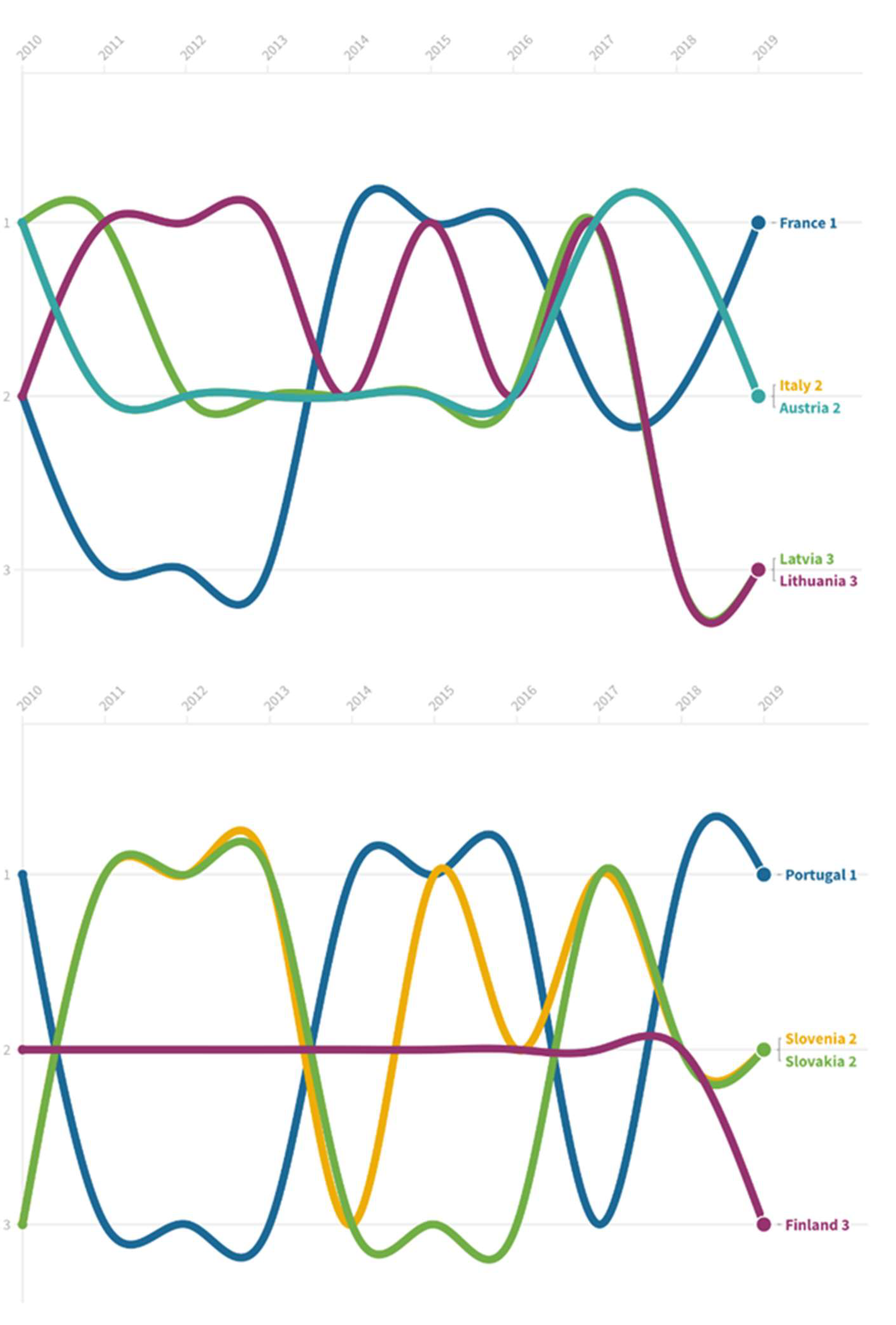
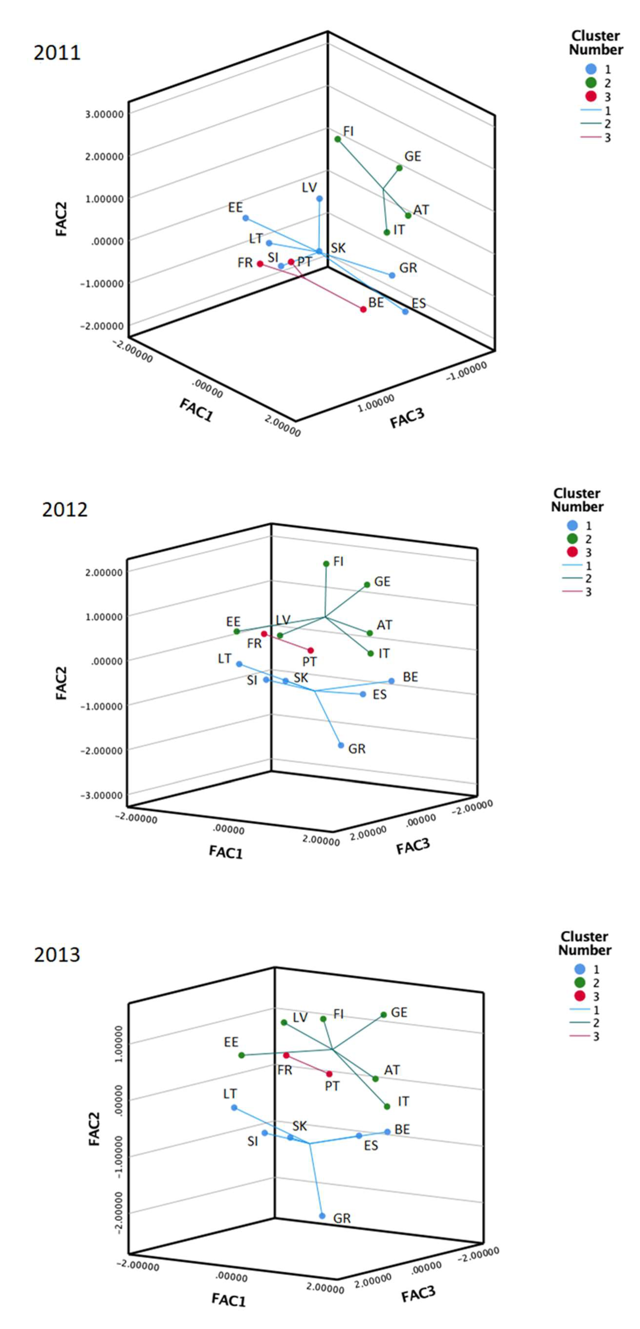
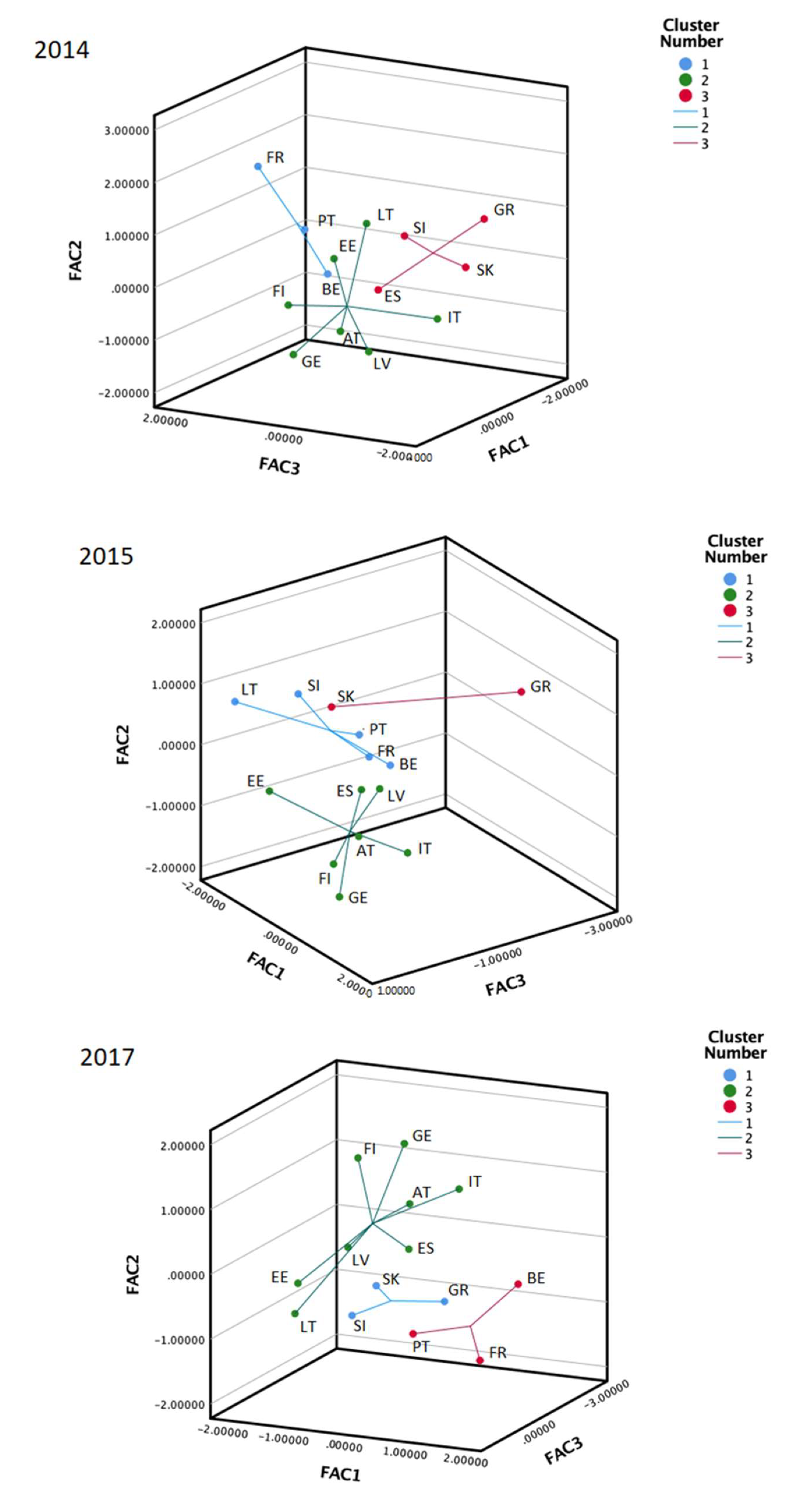
The other annual three-cluster cases (Figure A1) and the timelines for the three-cluster case (Figure A2) can be seen in Appendix B.

The research covered the relationship between the position of budgets and the clustering of financial instruments.

If we cluster countries according to HICP, public debt-to-GDP, budgetary deficit, convergence interest rates and current account deficit we have different outliers than using financial portfolio statistics. The outliers in 2010 were Ireland, Portugal, Greece, Latvia (this latter was because of extreme inflation data), in 2013 Greece and Slovenia, in 2016 Greece and Cyprus and in 2019 Greece and Italy. In 2010, the rest of the countries remained relatively homogeneous. In 2013, Germany, Luxembourg and the Netherlands came away from the rest, and in 2016 the same countries detached from the others plus most of the countries joining after 2000 lived separate lives as well. Finally, in 2019, Ireland, Portugal and Cyprus started forming a new group after filtering out individual outliers, the rest remained rather homogeneous.

Novák and Tatay (2021b) carried out a cluster analysis using a mixture of financial asset and macroeconomic variables, and using budgetary deficit among the variables defining the various clusters. They concluded that, due to the low interest rates, variables capturing portfolio rearrangements supported the countries’ convergence (at least as concerns older and newer eurozone members), though the adjustment happened partly by the accumulation of more liquid assets and partly by favoring equity investment and insurance technical reserves among the countries examined.

Following on Novák and Tatay (2021b), it is easy to observe that clustering countries by budget deficit/public debt and debt securities results in a very similar grouping of countries, which is especially apparent if we use household holdings of debt securities. Calculating correlations, however, resulted in diminishing correlations, between 2010 and 2019, between government debt-to GDP and debt securities holdings of the economies.

The authors have examined the government deficits throughout all clusters and time periods.

Table 1. The average and standard deviations of government deficits.

	2010		2011		2012		2013
	Average	Std. Dev.	Average	Std. Dev.	Average	Std. Dev.	Average	Std. Dev.
Cluster 1	−9.075	3.53	−6.17	4.06	−6.1	3.41	−7.35	5.47
Cluster 2	−4.82	2.26	−2.03	1.31	−1.5	1.15	−1.4	1.29
Cluster 3	−5.34	3.17	−5.73	1.76	−5.6	0.84	−4.6	0.7
Kruskal-Wallis test sig.	0.205		0.075		0.008		0.015
Post hoc test between 2 clusters
CL. 1 and Cl. 2					0.017		0.021
Cl. 1 and Cl. 3					0.696		0.942
Cl. 2 and Cl. 3					0.057		0.144
Year	2014		2015		2016		2017
	Average	Std. Dev.	Average	Std. Dev.	Average	Std. Dev.	Average	Std. Dev.
Cluster 1	−4.8	2.29	−2.7	1.55	−2.63	0.87	−0.17	0.8
Cluster 2	−1.37	1.63	−1.66	2.06	−1.19	1.66	−0.82	1.4
Cluster 3	−4.58	1.45	−4.3	2.26	−1.2	1.98	−2.23	1.32
Kruskal-Wallis test sig.	0.007		0.174		0.316		0.3
Post hoc test between 2 clusters
CL. 1 and Cl. 2	0.039
Cl. 1 and Cl. 3	0.927
Cl. 2 and Cl. 3	0.026
Year	2018		2019
	Average	Std. Dev.	Average	Std. Dev.
Cluster 1	0.2	1.75	−1.5	2.26
Cluster 2	−1.17	1.02	−0.17	1.4
Cluster 3	−0.67	1.09	−0.8	1.4
Kruskal-Wallis test sig.	0.325		0.484

Source Authors’ calculation.

shows the averages and standard deviations of government deficits for each year and each cluster, according to the reduced class of the countries (14 countries in the examination).

Since the cluster sample sizes were small, between 2 and 9, the condition of normal distribution could not be guaranteed. Therefore, we applied the Kruskal-Wallis nonparametric statistical test in order to examine if there was a significant difference in means between the clusters regarding government deficits. The significance level was 0.05. Significance values were adjusted by the Bonferroni correction for multiple tests. If the Kruskal-Wallis test showed significant difference between the clusters in a specified year, we indicated the results of the pairwise comparisons of the clusters for that year (2012, 2013, and 2014). Based on the results, we could say that there was significant difference in means between the clusters only in years 2012, 2013 and 2014, the period of the petering out of the sovereign debt crisis. In all of these years the second cluster (Germany, Estonia, Italy, Latvia, Austria, Finland, and Lithuania in 2014) showed significantly smaller government deficit than the other two clusters. The cluster with the lowest deficit values corresponded to the more balanced cluster based on the principal components at the same time.

The results confirmed that euro area financial markets were fragmented. There were significant differences in the stock of financial assets across countries before the ECB cut the base rate to the zero level. Clustering components were total cash holdings and transferable deposits. In the low interest rate environment, money holdings were becoming more significant, but their share of GDP differed across countries. Within each cluster, core countries and periphery countries were also found in different groups. The movement over time between the core and periphery country groups was not entirely unidirectional. However, an assessment of the time course showed that the launch of QE led to different movements between clusters than the monetary policy that had previously operated only by lowering interest rates. This result was also similar to empirical data analyses in previous literature. On the other hand, in the cluster analysis of this paper supplementing previous research findings, the fragmentation of euro area financial markets was assessed by the evolution of financial aggregates based on Keynes’ liquidity preference theory.

5. Materials and Methods

The paper uses k-centers cluster analysis based on Euclidean distance for detecting changes in the portfolio holdings of eurozone economic actors owing to economic crises and monetary policy responses.

The rationale behind the use of cluster analysis is to detect any change in the evolution of clusters in the eurozone within the member states as a result of the changing monetary policy. Similar cluster analysis was carried out by Danko and Suchỳ (2021) on the capital market integration of European economies, but this study did not discuss the importance of monetary policy decisions. Cluster analysis can capture well the change of country groupings based on portfolio decisions of economic actors, but cannot explain the responses of individual countries to the various monetary policy steps taken. Therefore, the selected methodology has its shortcomings in explaining the effect of monetary policy, in that it is not able to present impulse responses to internal monetary policy decisions or external shocks. Thus, the cluster analysis applied within this paper allows only for the changing participation of countries in the various clusters defined by the most important portfolio assets with which the principal components most strongly correlate.

In this study, the annual GDP-proportionate total economic financial assets data were retrieved from the Eurostat database for the period 2010 and 2019 for analysis. As a starter, data on investment into total assets, loans, currency, debt securities, transferable deposits, other deposits, equity, investment funds and insurance, pension and guarantee funds were examined with the help of principal component analysis. The principal components were standardized and subject to Kaiser-Meyer-Olkin measure to check the suitability of the data series to the factor analysis. Three components were identified to condense the information in the dataset, applying the varimax rotation. The first principal component resulting this way had a strong connection to most of the financial assets, apart from currency, deposits and insurance technical reserves. The second principal component condensed information, mostly from deposits and/or debt securities, and the third had high correlation with currency, often having a negative relationship with the third component. The content of the components, however, changed from one year to the other and depended on the sample data coverage.

First, all the 19 countries were subject to cluster analysis over the period considered by keeping Luxembourg as the biggest outlier within the group of countries examined. This method helped to understand the evolution of clusters over time. When keeping all the countries in the sample, including Luxembourg, as forming a separate group over the entire time period, the Kaiser-Meyer-Olkin measure showed very low values for the principal components identified this way. Then, dividing the selected countries into two clusters, while casting off Luxembourg, helped detect each major move of the individual countries from one cluster to another within a two-cluster framework. Finally, all the major outliers, including Cyprus, Malta, Luxembourg, Ireland and the Netherlands, were excluded from the sample and an annual three-cluster examination was carried out. The Kaiser-Meyer-Olkin measure took values above 0.5, or, in some years, even above 0.6 for the truncated samples. For a better illustration of the changing composition of clusters timelines, Sankey representations and three-dimensional diagrams (where each axis indicated the particular principal component value) were applied. All the calculations and illustrations were conducted with the help of IBM SPSS 28.

6. Conclusions

We assumed the fragmentation of financial markets in euro area economies. Based on Keynes’ liquidity preference theory, we assumed that the liquidity trap phenomenon would lead to a change in the structure of financial asset holdings of the countries concerned, due to the ECB’s policy of interest rate cuts. Due to the fragmented nature of their financial markets, we assumed that the structure of the change would be different in each country. We wanted to show the fragmentation precisely by showing the changes in portfolio structures from different aspects.

For our analysis we used cluster analysis as a method, by using asset data series from the Eurostat database. When the clusters were formed, five of the euro area countries showed strikingly different pictures. These were Ireland, Cyprus, Luxembourg, Malta and the Netherlands. These outliers were likely to behave in a very distinguishable nature, due to their specific balances of payments resulting from their specific tax rules. Excluding these outliers, the data for the other countries were further analyzed.

The remaining 14 countries could be split into three distinct clusters throughout the period 2010–2019. Total financial assets, transferable deposits, short-term debt and currency were the main components used to form the clusters. The clustering was, therefore, carried out along three dimensions capturing these characteristics with the help of principal components. Our hypothesis proved to be valid with respect to the fragmentation of the euro area financial markets. At the same time, in line with the liquidity preference theory, agents in the economies changed their portfolio and, in general, moved to more currency and less debt securities holdings. Overall, however, there was evidence for money demand becoming higher after 2015, as transferable deposits remained and even grew in importance as portfolio components for countries such as Germany, Finland, Austria and Italy, while, among the rest of the countries, especially in Spain, a positive move was mostly perceptible as well.

It is important to emphasize, however, that the changing portfolio structure of the eurozone economies in the period considered, full of financially turbulent subperiods, such as the aftermath of the global financial crisis, the sovereign debt crisis and some financial anomalies already present preceding the 2020 COVID 19 crisis, cannot only be explained by concrete monetary policy decisions and the declining yield curve. Apart from some traditional investment preferences, that economic actors of the selected countries could be characterized by, especially the household sectors, it is important to note that the financial sector’s investment decisions were largely influenced by international liquidity and risk conditions, especially those deriving from US market tensions (see, among others, Sifat et al. 2022). Moreover, it has also been justified in the empirical literature that the asset structure of the financial sector and, therewith, the sources of systemic risk were strongly related to the general financing structure of the economy, whether it was more capital market-based or bank-based (Qin and Zhou 2019). On the other hand, uncertainty around monetary policy decisions, especially discernible under the zero lower bound, had a notable impact on the yield curve and the effectiveness of monetary policy easing or tightening (Tillmann 2020), especially if one considers that policy uncertainty from the US could have a greater effect on European economies than that perceived in Europe itself (Colombo 2013). Therefore, our results should also be placed in an international context, in a period with strongly deviating monetary policies.

At the same time, in line with the liquidity preference theory, agents in the economies changed their portfolio and, in general, moved to more currency and less debt securities holdings, Greece being the most apparent example of behaving the opposite way and, thus, converging to average levels. Overall, there was evidence for money demand becoming higher after 2015, as transferable deposits remained and even grew in importance as portfolio components for countries such as Germany, Finland, Austria and Italy, while, among the rest of the countries, especially in Spain, a positive move was mostly perceptible as well. In some countries, the adjustment of investors’ preferences resulted in a move to more equity securities and investment fund shares instead of simply accumulating more liquid (non-interest paying) instruments, as Novák and Tatay (2021b) conjectured. These portfolio restructuring decisions happened despite the dissimilar monetary policy steps taken by the Fed and the ECB, as the Fed gave up the zero lower bound as soon as the end of 2015. At the same time, it was also generally observable that, while the sovereign debt crisis occurred, during which the ECB only marginally resorted to asset purchases and more to long-term refinancing operations, and did not cut the policy rate to zero, fiscal policy was a much more important aspect for portfolio decisions (as justified by the evolution of the various clusters and the investment into debt securities) than after 2015. After 2015 QE became a more characteristic tool of the ECB and the base rate was cut effectively to zero and we found no statistical evidence for the relationship between investment decisions and fiscal policy variables. Despite some convergence and generally observable tendencies, like in the “central cluster” with Germany in the nucleus, as Danko and Suchỳ (2021) also pointed out, the common monetary policy was conducted in an economic environment with a rather diverse portfolio structure during the low interest rate environment and the inhomogeneity of member states, suggested by the literature, gained further justification.

The analysis showed that the ECB’s monetary policy does not have a uniform impact on euro area financial markets, having different effects in the economies concerned. Moreover, the use of different monetary policy instruments also modifies these differences.

A further line of research could be to examine the financial asset holdings of each sector of economic agents individually, with a focus on the portfolio decisions of households.

References

1. Acharya, Viral V., Itamar Drechsler, and Philipp Schnabl. 2012. A tale of two overhangs: The nexus of financial sector and sovereign credit risks. Financial Stability Review 16: 51–56. [Google Scholar]
2. Agba, Eli, Hamza Bennani, and Jean-Yves Gnabo. 2022. Assessing the sources of heterogeneity in eurozone response to unconventional monetary policy. Applied Economics 54: 5549–74. [Google Scholar] [CrossRef]
3. Andreeva, Desislava C., and Miguel García-Posada. 2021. The impact of the ECB’s targeted long-term refinancing operations on banks’ lending policies: The role of competition. Journal of Banking and Finance 122: 105992. [Google Scholar] [CrossRef]
4. Backhouse, Roger E. 2020. Economic theory in an imperfect world: Frank Hahn, general equilibrium, and Keynesian economics. Oxford Economic Papers 72: 1091–107. [Google Scholar] [CrossRef]
5. Barens, Ingo. 2018. Robertson’s ‘Liquidity Trap’as an Answer to Keynes’s ‘Banana Parable’, or: Did the General Theory Really Have to Be Written. Paper present at the ESHET Conference, Madrid, Spain, September 7–9. [Google Scholar]
6. Bibow, Jorg. 2013. Keynes on Monetary Policy, Finance and Uncertainty: Liquidity Preference Theory and the Global Financial Crisis. New York: Routledge. [Google Scholar]
7. Boianovsky, Mauro. 2004. The IS-LM model and the liquidity trap concept: From Hicks to Krugman. History of Political Economy 36: 92–126. [Google Scholar] [CrossRef] [Green Version]
8. Brady, Michael Emmett. 2018. Keynes’s March 31, 1937 Message to Hicks About the IS-LM Model: ‘At One Time I Tried the Equations, as You Have Done, with I in All of Them’. [CrossRef]
9. Brunner, Karl, and Allan H. Meltzer. 1968. Liquidity traps for money, bank credit, and interest rates. Journal of Political Economy 76: 1–37. [Google Scholar] [CrossRef] [Green Version]
10. Caballero, Ricardo J., and Emmanuel Farhi. 2018. The safety trap. The Review of Economic Studies 85: 223–74. [Google Scholar] [CrossRef]
11. Cardim de Carvalho, Fernando J. 2010. Uncertainty and money: Keynes, Tobin and Kahn and the disappearance of the precautionary demand for money from liquidity preference theory. Cambridge Journal of Economics 34: 709–25. [Google Scholar] [CrossRef]
12. Colombo, Valentina. 2013. Economic policy uncertainty in the US: Does it matter for the Euro area? Economics Letters 121: 39–42. [Google Scholar] [CrossRef] [Green Version]
13. Cook, David, and Michael B. Devereux. 2011. Optimal fiscal policy in a world liquidity trap. European Economic Review 55: 443–62. [Google Scholar] [CrossRef]
14. Danko, Jakub, and Erik Suchỳ. 2021. The financial integration in the European capital market using a clustering approach on financial data. Economies 9: 89. [Google Scholar] [CrossRef]
15. Dantas, Manuela, Kenneth J. Merkley, and Felipe Bastos G. Silva. 2022. Government Guarantees and Banks’ Income Smoothing. Available online: https://papers.ssrn.com/sol3/papers.cfm?abstract_id=2797697 (accessed on 7 August 2022).
16. Dedola, Luca, Georgios Georgiadis, Johannes Gräb, and Arnaud Mehl. 2021. Does a big bazooka matter? Quantitative easing policies and exchange rates. Journal of Monetary Economics 117: 489–506. [Google Scholar] [CrossRef]
17. Gori, Filippo. 2018. Banking integration and monetary policy fragmentation in the Eurozone. International Economics and Economic Policy 15: 131–57. [Google Scholar] [CrossRef]
18. Havlik, Annika, Friedrich Heinemann, Samuel Helbig, and Justus Nover. 2022. Dispelling the shadow of fiscal dominance? Fiscal and monetary announcement effects for euro area sovereign spreads in the corona pandemic. Journal of International Money and Finance 122: 102578. [Google Scholar] [CrossRef]
19. He, Zhiguo, and Arvind Krishnamurthy. 2013. Intermediary asset pricing. American Economic Review 103: 732–70. [Google Scholar] [CrossRef] [Green Version]
20. Hicks, John R. 1937. Mr. Keynes and the ”classics”; a suggested interpretation. Econometrica: Journal of the Econometric Society 5: 147–59. [Google Scholar] [CrossRef]
21. Hicks, John R. 1942. The monetary theory of DH Robertson. Economica 9: 53–57. [Google Scholar] [CrossRef]
22. Hicks, John R. 1974. Crisis in Keynesian Economics. Oxford: Basil Blackwell. [Google Scholar]
23. Horvath, Roman. 2018. Financial market fragmentation and monetary transmission in the euro area: What do we know? Journal of Economic Policy Reform 21: 319–34. [Google Scholar] [CrossRef]
24. Horváth, Dániel, and Róbert Szini. 2015. The safety trap–the financial market and macroeconomic consequences of the scarcity of safe assets. Financial and Economic Review 14: 111–38. [Google Scholar]
25. Ijtsma, Pieter, Laura Spierdijk, and Sherrill Shaffer. 2017. The concentration–stability controversy in banking: New evidence from the EU-25. Journal of Financial Stability 33: 273–84. [Google Scholar] [CrossRef]
26. Itoh, Motoshige, and Naoki Shimoi. 2000. On the role of monetary policy in a deflationary economy: The case of Japan. Journal of the Japanese and International Economies 14: 238–60. [Google Scholar] [CrossRef]
27. Kahn, Richard Ferdinand. 1972. Notes on the Rate of Interest and the Growth of Firms. In Selected Essays on Employment and Growth. New York: Cambridge University Press, pp. 208–32. [Google Scholar]
28. Karadima, Maria, and Helen Louri. 2020. Bank competition and credit risk in Euro area banking: Fragmentation and convergence dynamics. Journal of Risk and Financial Management 13: 57. [Google Scholar] [CrossRef] [Green Version]
29. Keynes, John Maynard. 1936. The General Theory of Employment, Interest and Money. Cambridge: Macmillan Cambridge University Press. [Google Scholar]
30. Kiley, Michael. 2018. Quantitative easing and the ‘new normal’ in monetary policy. The Manchester School 86: 21–49. [Google Scholar] [CrossRef]
31. Krugman, Paul R., Kathryn M. Dominquez, and Kenneth Rogoff. 1998. It’s baaack: Japan’s slump and the return of the liquidity trap. In Brookings Papers on Economic Activity. Washington: The Brookings Institution, vol. 29, pp. 137–205. [Google Scholar]
32. Kuroda, Haruhiko. 2016. Quantitative and Qualitative Monetary Easing (QQE) with Yield Curve Control: New Monetary Policy Framework for Overcoming Low Inflation. Paper presented at the Speech at Brookings Institution in Washington DC on 8 October 2016, Washington, DC, USA, October 8; p. 8. [Google Scholar]
33. Lhuissier, Stéphane, Benoît Mojon, and Juan Francisco Rubio-Ramirez. 2020. Does the Liquidity Trap Exist? BIS Working Papers No. 855. Available online: https://www.bis.org/publ/work855.htm (accessed on 10 August 2022).
34. Lucotte, Yannick. 2015. Euro area banking fragmentation in the aftermath of the crisis: A cluster analysis. Applied Economics Letters 22: 1046–50. [Google Scholar] [CrossRef]
35. McCallum, Bennett. 2000. Theoretical Analysis Regarding a Zero Lower Bound on Nominal Interest Rates. Cambridge: National Bureau of Economic Research Cambridge. [Google Scholar]
36. Meltzer, Allan H. 1999. Commentary: Monetary Policy at Zero Inflation. Paper presented at the Jackson Hole Economic Policy Symposium: New Challenges for Monetary Policy, Kansas City, MO, USA, August 26–28; pp. 261–76. [Google Scholar]
37. Novák, Zsuzsanna, and Tibor Tatay. 2021a. ’Captivated by Liquidity’–Theoretical Traps and Practical Mazes. Pénzügyi Szemle/Public Finance Quarterly 66: 50–67. [Google Scholar] [CrossRef]
38. Novák, Zsuzsanna, and Tibor Tatay. 2021b. Liquidity trap or portfolio diversity. In XV. Financial Days Conference of Sopron, Sustainable Economy—Sustainable Finances” Professional and Scientific Conference on Finance, Taxation and Accounting. Edited by Kovács Tamás and Szóka Károly. Sopron: A Soproni Felsőoktatásért Alapítvány, pp. 226–236. [Google Scholar]
39. Patinkin, Don. 1974. The role of the “liquidity trap” in Keynesian economics. PSL Quarterly Review 26: 108. [Google Scholar]
40. Qin, Xiao, and Chunyang Zhou. 2019. Financial structure and determinants of systemic risk contribution. Pacific-Basin Finance Journal 57: 101083. [Google Scholar] [CrossRef]
41. Robertson, Dennis Holme. 1940. Essays in Monetary Theory. London: Staples Press. [Google Scholar]
42. Runde, Jochen. 1994. Keynesian uncertainty and liquidity preference. Cambridge Journal of Economics 18: 129–44. [Google Scholar]
43. Sargent, Thomas J. 1999. A primer on monetary and fiscal policy. Journal of Banking & Finance 23: 1463–82. [Google Scholar] [CrossRef]
44. Sifat, Imtiaz, Alireza Zarei, Seyedmehdi Hosseini, and Elie Bouri. 2022. Interbank liquidity risk transmission to large emerging markets in crisis periods. International Review of Financial Analysis 82: 102200. [Google Scholar] [CrossRef]
45. Silva, Felipe Bastos Gurgel. 2021. Fiscal Deficits, Bank Credit Risk, and Loan-Loss Provisions. Journal of Financial and Quantitative Analysis 56: 1537–89. [Google Scholar] [CrossRef]
46. Tatay, Blanka, and Tibor Tatay. 2020. Analysis of the causes of economic stagnation in Japan. Gazdaság & Társadalom 13: 21–42. [Google Scholar]
47. Tillmann, Peter. 2020. Monetary policy uncertainty and the response of the yield curve to policy shocks. Journal of Money, Credit and Banking 52: 803–33. [Google Scholar] [CrossRef]
48. Tobin, James. 1947. Liquidity preference and monetary policy. The Review of Economics and Statistics 29: 124–31. [Google Scholar] [CrossRef]
49. Tobin, James. 1971. Essays in Economics: Volume 1: Macroeconomics. Amsterdam: North-Holland Publishing Company. [Google Scholar]
50. Ueda, Kazuo. 2001. Japan’s Liquidity Trap and Monetary Policy’. Paper presented at the Speech to the Japan Society of Monetary Economics, Fukushima University, Fukushima, Japan, September 29; p. 29. Available online: https://www.boj.or.jp/en/announcements/press/koen_2001/ko0112a.htm/ (accessed on 20 September 2021).
51. Vari, Miklos. 2015. Implementing Monetary Policy in a Fragmented Monetary Union. Available online: https://ideas.repec.org/p/bfr/banfra/529.html (accessed on 1 July 2022).
52. Werner, Richard A. 2005. The Enigma of the Ineffectiveness of Interest Rate Policy in the 1990s. In New Paradigm in Macroeconomics. New York: Palgrave Macmillan, pp. 49–77. [Google Scholar]
Figure 1. Euro yield curves-annual data 2010–2019 (euro area). Source: Authors’ construction using database of Eurostat.
Risks 10 00192 g001
Figure 2. Sankey representation of cluster moves. Source Authors’ construction.
Risks 10 00192 g002
Figure 3. (ac) The detailed timeline of clusters for the two-cluster and 18 countries cases. Source Authors’ construction.
Risks 10 00192 g003aRisks 10 00192 g003b
Figure 4. The “truncated” three-cluster case in 2010. Source Authors’ construction.
Risks 10 00192 g004
Figure 5. The “truncated” three-cluster case in 2016. Source Authors’ construction.
Risks 10 00192 g005
Figure 6. The “truncated” three-cluster case in 2019. Source Authors’ construction.
Risks 10 00192 g006