Optimal Liquidation, Acquisition and Market Making Problems in HFT under Hawkes Models for LOB

Abstract

The present paper is focused on the solution of optimal control problems such as optimal acquisition, optimal liquidation, and market making in relation to the high-frequency trading market. We have modeled optimal control problems with the price approximated by the diffusion process for the general compound Hawkes process (GCHP), using results from the work of Swishchuk and Huffman. These problems have been solvedusing a price process incorporating the unique characteristics of the GCHP. The GCHP was designed to reflect important characteristics of the behaviour of real-world price processes such as the dependence on the previous process and jumping features. In these models, the agent maximizes their own utility or value function by solving the Hamilton–Jacobi–Bellman (HJB) equation and designing a strategy for asset trading. The optimal solutions are expressed in terms of parameters describing the arrival rates and the midprice process from the price process, modeled as a GCHP, allowing such characteristics to influence the optimization process, aiming towards the attainment of a more general solution. Implementations of the obtained results were carried out using real LOBster data.

1. Introduction

High-frequency trading was developed in the 1990s in response to advances in computer technology and the adoption of this new technology by exchanges. From the original rudimentary order processing approach to the current state-of-the-art all-inclusive trading systems, high-frequency trading (HFT) has evolved into a billion-dollar industry (Aldridge 2009). HFT is not merely electronic trading; it especially involves programming an algorithm that optimizes the timing and routing of the order in the limit order book (LOB).

High-frequency trading models have developed along with the technology surrounding those markets, especially the stochastic process models that have been used to represent those variables, given their malleability in approaching the dynamics of the assets in the best way possible. This analysis has been mostly framed in a continuous time with the aim of ensuringthe speed of the transactions in those markets (which is generally measured in nanoseconds).

Among the issues involved in HFT, optimal control problems such as optimal acquisition, optimal liquidation, and market making are among the most important. These problems have been addressed previously by many authors and in this section of this working paper, we present a review of the relevant literature on the construction of models in relation to limit order markets.

In the following, we present a brief description of the mechanism of LOB, as detailed in Cartea et al. (2015). First of all, there are orders to buy and sell assets that arrive at an exchange. There are three types of orders:

• Market buy/sell order—specifies the number of shares to be bought/sold at the best available price, immediately.
• Limit buy/sell order—specifies a price and a number of shares to be bought/sold at that price, when possible.
• Order cancellation—agents who have submitted a limit order may cancel the order before it is executed.

Regarding these types of orders, there are:

• Market orders that are executed immediately.
• Limit orders that are queued for later execution, but which may be canceled.
• Thus, the limit-order book is the collection of queued limit orders awaiting execution or cancellation.

The bid price $S_t^b$ is the highest limit buy order price in the book. It is the best available price for a market sell. The ask price $S_t^a$ is the lowest limit sell order price in the book. It is the best available price for a market buy. In general, we are interested in the midprice:

$$S_t:=(S_t^b+S_t^a)/2.$$

It is worth noting that the tick size ($\delta$) of an LOB is the smallest permissible price interval between different orders within it. All orders must arrive with a price that is specified to the accuracy of $\delta$.

According to the arrival of the market orders, the modeling of the midprice has to reflect sudden movements such jumps in stock prices inside the limit order markets. The Markov process has been used to simulate the behavior of the price in a limit order book (LOB, the place where every transaction is negotiated). Lèvy processes, such as the compound Poisson process, have been implemented in modeling stock dynamics, such as in a study by Merton (1976). The Poisson process has the following strong characteristics: the arrival of an event is independent of the previous event (the waiting time between events is memoryless), the average rate is constant, and two events cannot be simultaneous. In reality, many phenomena modeled as Poisson processes do not meet these attributes exactly. Thus, numerous analysts have examined sudden price jumps and amplified them to make them follow more general Markov processes.

In a study by Cont and Larrard (2013), the arrival orders in an LOB were described in terms of Markovian processes. The authors proposed a Markovian model of a limit order market, which captured the autocorrelation of price changes. Their model linked price changes and the duration until the next price change.The authors computed the conditional distributions of durations and price changes, and presented analytical results supporting their theory in which these two factors are not independent, as they are assumed to be in the compound Poisson process.Finally, they remarked that high-frequency increments of the price were negatively correlated, meaning that an increase in price would probably be followed by a decrease in price.

Subsequently, Swishchuk and Vadori (2017) used the Markov renewal process to model an LOB. The authors performed an extension of the model presented in the work of Cont and Larrard (2013), changing two main aspects: first, the interarrival times of book events were allowed to have an arbitrary distribution (previously these were assumed to be exponential, as in the Poisson process, but evidence shown in the numerical results discussed in this paper showed these to be non-exponential), and second, the interarrival times of new book events could depend on the nature of previous events (these were formerly assumed to be independent), which was reflected in the numerical results seen in LOBster data (LOBster 2012) (see Section 6.2). This change in assumptions was possible given the nature of the Markov renewal process. Furthermore, in a study by Swishchuk et al. (2017), the authors applied the use of general semi-Markov models to an LOB in order to make LOB models more flexible. They incorporated price changes that were not fixed to one tick, in contrast to the Poisson assumption that two events cannot be simultaneous. This implementation was also justified with numerical results obtained from different limit order book data, including LOBster data (LOBster 2012).

In the search for models that can accurately reflect the behaviour of high-frequency financial data, Hawkes processes have been applied to address many different problems in high-frequency finance, as discussed in the work of Bacry et al. (2015). Hawkes processes are a particular class of multivariate point processes with specific characteristics: they are self-exciting, with clustering effects and long-run memory. Hawkes processes with a certain structure have Markovian properties (Bacry et al. 2015), and a Poisson process can be expressed as a particular Hawkes process. Hawkes process characteristics have been provento exist in financial data. As mentioned previously, the Poisson process assumed independence in the arrival of events, in contrast with the Hawkes process with its dependence on history. This is also what was removed from the price process models in previous Markov and semi-Markov models. Boswijk et al. (2018) extended the notion of self-excitation in jumps and detected its presence in a discretely observed sample path at high frequency. Lu and Abergel (2017, 2018) modeled an LOB with a high-dimensional Hawkes process and found good agreement between the statistical properties of the LOB data and the model. Subsequently, Liu et al. (2021) studied the optimization problem of a household under the influence of a contagious financial market, using the clustering effect property of the Hawkes process.

Swishchuk and Huffman (2020) studied general compound Hawkes processes to model the price process in LOBs. The authors proved a law of large numbers (LLN) and a functional central limit theorem (FCLT) for some cases of these processes. Specifically, they proved those theorems for an asymptotic analysis of the general compound Hawkes process with two state-dependent orders.To obtain empirical results, they used LOBster data (LOBster 2012) to calibrate the parameters of these asymptotic models. The interarrival times and clustering effect were analyzed to prove that the prices in the LOBster dataset were not following the Poisson process, so this approach was consistent with Hawkes modeling. The relevance of the multivariate general compound Hawkes process (MGCHP) in LOBs was analyzed by Guo and Swishchuk (2020) and Guo et al. (2020), who provided awareness about price volatilities in LOBs for several assets using real-world data.

Therefore, these papers provided us with a basis for adopting the general compound Hawkes process and its unique properties for modeling the midprice, $S_t$, in the stochastic optimal control problems, given that it provides a better description of real-life data in high-frequency trading.

The authors of another study (Fodra and Pham 2015) built a bridge between the two main streams of literature in high-frequency trading models of intra-day asset prices and high-frequency trading problems. The authors described the stock price through a pure jump process. The process $P_t$ was embedded into the Markov system with three observable state variables: $(P_t,I_t,S_t)$, a Markov renewal process with a known infinitesimal generator, obtained from the infinitesimal generator of $(P,I,S)$, and the dynamics of the controlled process of wealth and inventory.They were able to solve the Hamilton–Jacobi–Bellman (HJB) equation through dynamic programming, associated with the control problem of maximization of utility.After obtaining this equation, the authors were able to provide an interesting financial interpretation of their results, decomposing the results into the trading portion (small orders with no impact on price) and the jump portion (large orders producing a jump in the price level).

Following Fodra and Pham (2015), we can obtain diffusion results: the stock price process $S_t$, modeled using the GCHP, can be approached with a stochastic differential equation (SDE) of the price, as well as the infinitesimal generator. In this paper, the price is approximated by means of diffusion models, using the law of large numbers (LLN) and the functional central limit theorem (FCLT) for the general compound Hawkes process (GCHP), incorporating results from Swishchuk and Huffman (2020).

Subsequently, we solve optimal control problems, such as optimal acquisition, optimal liquidation, and market making, related to the high-frequency trading market. Previous researchers (Cartea et al. 2015) have developed mathematical tools for the analysis of trading algorithms used on stochastic optimal control problems in a very general way, which we apply to solving the optimization problem in the present work. Furthermore, the authors in Cartea et al. (2015) attempted the modeling of diverse algorithmic trading strategies. Liquidate and acquire modelswere constructed to execute a large position using market orders, using a price model of the general stationary Gauss–Markov process. In Becherer et al. (2018), the authors explicitly determined the optimal liquidation of an asset position using a price model of a controlled Ornstein–Uhlenbeck process in a financial market with multiplicative and transient price impacts. Market-making models presented in in Cartea et al. (2015) were used to maximize the market maker’s profit by choosing the depth at which to place the limit orders. In Fruth et al. (2019) the authors modeled a limit order book with stochastic liquidity to explain random variations in the depth of the order book and evaluate their influence on optimal trade execution strategies, using the price model of the Cox–Ingersoll–Ross model. The innovative solutions discussed in this research work come from assuming that the midprice can be approximated by the diffusion process of the GCHP, which has the property of being more flexible and therefore more able to fit with real-life prices.

The models used in this study describe the controlled inventory process $Q_t$ of the agent, the midprice with the corresponding SDE, the cash process $X_t$ of the agent, in order to evaluate the agent’s value function $H(t,x,S,q)$. To solve this optimal control problem, the dynamic programming equation (DPE) was developed. This is also known in this context as the Hamilton–Jacobi–Bellman equation, which is satisfied by the value function H that can be obtained by observing at the dynamic programming principle (DPP). The final results are the optimal inventory $Q_t^{*}$, the optimal speed of trading ${\nu }_t^{*}$, and the optimal depth ${\delta }^{*,\pm }(t,q)$. The optimal solutions are expressed in terms of parameters describing the arrival rates and the midprice, modeled as a GCHP. By allowing these characteristics influence the optimization process, we have developed a more general solution that describes in a more authentic manner the observed price process in HFT markets.

The present paper is organized as follows. Section 2 provides a brief introduction to Hawkes processes. Section 3, Section 4 and Section 5 describe the optimal liquidation processes for liquidation, acquisition, and market making, respectively, as well as presentingthe models proposed for the price process, main characteristics, the SDE equation, the structure of their infinitesimal generator, the approach used to solve the HJB equations for the optimal control problems, a characterization of the pathway to solving these problems, and a closed solution for these problems. Section 6 shows the manner in which these solutions work when applied to real life data. Section 7 presents our conclusions regarding the study’s results, and in Section 8 we discuss these results, as well as future research directions.

2. A Brief Introduction to Hawkes Processes

The Hawkes process (HP) is named after its creator, Alan Hawkes (1971). We can describe the HP process $N\left(t\right)$ as a counting process that has a self-exciting property, a clustering effect, and long-runmemory properties, which are consistent with what it has been observed in the empirical data on limit order books (Swishchuk and Huffman 2020).

Definition 1

(One-dimensional Hawkes Process (Hawkes and Oakes 1974)). The one-dimensional Hawkes process is a point process $N\left(t\right)$ which is characterized by its intensity $\lambda \left(t\right)$ with respect to its natural filtration:

$$\lambda \left(t\right)=\lambda +{\int }_0^t\mu (t-s)dN\left(s\right)$$

(1)

where $\lambda >0$, and the response function $\mu \left(t\right)$ is a positive function that satisfies ${\int }_0^{\infty }\mu \left(s\right)ds<1$.

The constant $\lambda$ is called the background intensity and the function $\mu \left(t\right)$ is called the excitation function.

Definition 2

((General Compound Hawkes Process with Two-State Dependent Orders) GCHP2SDO (Swishchuk and Huffman 2020)). Suppose that $X_k$ is an ergodic continuous time Markov chain, independent of $N\left(t\right)$, with state space $1,2$. Then, the general compound hawkes process with two states is defined by the following process

$$S_t=S_0+\sum _{k=1}^{N\left(t\right)}a\left(X_k\right)$$

(2)

where $a\left(X_k\right)$ takes only the values $a\left(1\right)$ and $a\left(2\right)$, $a\left(x\right)$ is a continuous and bounded function of $X=1,2$, and $N\left(t\right)$ is the number of price changes up to moment t, described by a one-dimensional Hawkes process defined in Definition 1.

This general model is rich enough to:

• Incorporate a non-exponential distribution of interarrival times of orders in HFT or claims in insurance (hidden in $N\left(t\right)$);
• Incorporate the dependence of orders or claims (via MC $X_i$);
• Incorporate the clustering of orders in HFT or claims (properties of $N\left(t\right)$); and
• Incorporate order or claim price changes that are different from one single number (in $a\left(X_i\right)$).

This model is also sufficiently general to include:

• Compound Poisson processes: $S_t=S_0+{\sum }_{k=1}^{N\left(t\right)}{X}_k,$ where $N\left(t\right)$ is a Poisson process and $a\left(X_k\right)=X_k$ are i.i.d.r.v.;
• Compound Hawkes processes (Swishchuk et al. 2019): $S_t=S_0+{\sum }_{k=1}^{N\left(t\right)}{X}_k,$ where $N\left(t\right)$ is a Hawkes process and $a\left(X_k\right)=X_k$ are i.i.d.r.v.; and
• Compound Markov renewal processes: $S_t=S_0+{\sum }_{k=1}^{N\left(t\right)}a\left(X_k\right),$ where $N\left(t\right)$ is a renewal process and $X_k$ is a Markov chain.

Lemma 1.

((LLN for GCHP) (Swishchuk and Huffman 2020)). Let $\widehat{\mu }:={\int }_0^{+\infty }\mu \left(s\right)ds$$<1,$ and assume that the Markov chain $X_i$ is ergodic with stationary probabilities ${\pi }_i^{*}.$ Then, the GCHP $S_{nt}$ satisfies the following weak convergence in the Skorokhod topology:

$$\frac{S\left(nt\right)}{n}{\to }_{n\to +\infty }{a}^{*}·\frac{\lambda }{1-\widehat{\mu }}t,$$

or

$$\frac{S\left(t\right)}{t}{\to }_{t\to +\infty }{a}^{*}·\frac{\lambda }{1-\widehat{\mu }}.$$

Here, $a^{*}$ is defined as $a^{*}:={\sum }_{i\in X}{\pi }_i^{*}a\left(i\right),$ where ${\pi }_i$ are ergodic probabilities for Markov chain $X_i.$

Theorem 1

((FCLT (or Jump-Diffusion Limit) for GCHP) (Swishchuk and Huffman 2020)). Let $X_k$ be an ergodic Markov chain and with ergodic probabilities $({\pi }_1^{*},{\pi }_2^{*},\dots ,{\pi }_n^{*}).$ Let $S_t$ be LGCHP, and $0<\widehat{\mu }:={\int }_0^{+\infty }\mu \left(s\right)ds<1and{\int }_0^{+\infty }\mu \left(s\right)sds<+\infty .$ Then

$$\frac{S\left(nt\right)-N\left(nt\right)·a^{*}}{\sqrt{n}}{\to }_{n\to +\infty }\sigma \sqrt{\lambda /(1-\widehat{\mu })}W\left(t\right),$$

in a weak sense for the Skorokhod topology, where $W\left(t\right)$ is a standard Wiener process, σ is defined as:

${\left(\sigma \right)}^2:={\sum }_{i\in X}{\pi }_i^{*}v\left(i\right)$

$$\begin{array}{ccc}\hfill v\left(i\right)& =& b{\left(i\right)}^2+\sum _{j\in X}{(g\left(j\right)-g\left(i\right))}^{2}P(i,j)\hfill \\ & -& 2b\left(i\right)\sum _{j\in X}(g\left(j\right)-g\left(i\right))P(i,j),\hfill \\ \hfill b& =& {(b\left(1\right),b\left(2\right),\dots ,b\left(n\right))}^{\prime },\hfill \\ \hfill b\left(i\right):& =& a\left(i\right)-a^{*},\hfill \\ \hfill g:& =& {(P+{\mathsf{\Pi }}^{*}-I)}^{-1}b,\hfill \end{array}$$

P is a transition probability matrix for $X_k,$ i.e., $P(i,j)=P(X_{k+1}=j|X_k=i),$${\mathsf{\Pi }}^{*}$ denotes the matrix of stationary distributions of $P,$ and $g\left(j\right)$ is the jth entry of $g.$ The expressions above are valid for both finite and infinite-state Markov chains; that is why we have used the notation ${\sum }_{j\in X},$ where X is the state space of an MC $X_i.$

Remark 1.

The formulas for $a^{*}$ and σ look much simpler in the case of a two-state Markov chain $X_i=\{-\delta ,+\delta \}:$

$$a^{*}:=\delta (2{\pi }^{*}-1)and{\left({\sigma }^{*}\right)}^2:=4{\delta }^2\left(\frac{1-p^{\prime }+{\pi }^{*}(p^{\prime }-p)}{{(p+p^{\prime }-2)}^2}-{\pi }^{*}(1-{\pi }^{*})\right),$$

$(p,p^{\prime })$ are transition probabilities of the Markov chain $X_k,$ and ${\pi }_1^{*}={\pi }^{*},{\pi }_2^{*}=1-{\pi }^{*}.$

From CLT for HP, (see (Swishchuk et al. 2019)) and from Theorem 1 presented above, the following FCLT can be observed for GCHP (pure jump diffusion limit).

Theorem 2

(FCLT (or Pure Diffusion Limit) for GCHP (Swishchuk and Huffman 2020)). Let $X_k$ be an ergodic Markov chain and with ergodic probabilities $({\pi }_1^{*},{\pi }_2^{*},\dots ,{\pi }_n^{*}).$ Let $S_t$ be LGCHP, and $0<\widehat{\mu }:={\int }_0^{+\infty }\mu \left(s\right)ds<1$ and ${\int }_0^{+\infty }\mu \left(s\right)sds<+\infty .$ Then

$$\frac{S\left(t\right)-a^{*}\frac{\lambda }{1-\widehat{\mu }}t}{\sqrt{t}}{\to }_{t\to +\infty }\overline{\sigma }N(0,1),$$

in weak sense for the Skorokhod topology, where $N(0,1)$ is the standard normal c.d.f., and $\overline{\sigma }$ is defined as:

$$\overline{\sigma }=\sqrt{{\left({\sigma }^{*}\right)}^2+{\left(a^{*}\sqrt{\frac{\lambda }{{(1-\widehat{\mu })}^3}}\right)}^2},$$

where ${\sigma }^{*}=\sigma \sqrt{\lambda /(1-\widehat{\mu })},$σ and $a^{*}$ are defined in Theorem 1 and the Lemma 1, respectively.

Remark 2.

Theorem 2 implies that $S\left(t\right)$ can be approximated by the pure diffusion process:

$$S\left(t\right)\approx S\left(0\right)+a^{*}\frac{\lambda }{1-\widehat{\mu }}t+\overline{\sigma }W\left(t\right),$$

where $W\left(t\right)$ is a standard Wiener process. Remark 2 expresses the ideaof the pure diffusion approximation of GCHP on a large time interval.

Remark 3.

We note that the rate of convergence in Theorem 2 is $C\left(T\right)/\sqrt{t},$$0\le t\le T,$ where $C\left(T\right)>0$ is a constant. Thus, the error of approximation for $S\left(t\right)$ in Remark 2 is very small for large $t.$

3. Optimal Liquidation Problem

One main concern in finance is how an agent can sell or buy a large amount of shares, while minimizing the adverse price movements of the asset traded. An amount is considered ‘large’ if the number of shares the agent seeks to execute is significantly larger than the average size of a trade. As these orders cannot be executed in one exhibition, the order will be sliced, and the time the agent takes to space out and execute the smaller orders is crucial (Cartea et al. 2015).

In this model of optimal liquidation, the agent posts market orders (MOs) to liquidate $\mathfrak{N}$ shares. The MOs are executed immediately at the midprice to liquidate the shares. In this direction, the agent’s orders affect the midprice with two possible impacts, a temporary and a permanent impact. To develop the optimal liquidation problem, the key stochastic processes can be described as follows:

• $\nu ={\left({\nu }_t\right)}_{\{0\le t\le T\}}$ is the trading rate, the speed at which the agent is liquidating or acquiring shares;
• $Q^{\nu }={\left(Q_t^{\nu }\right)}_{\{0\le t\le T\}}$ is the agent’s inventory, which is affected by the speed of trading;
• $S^{\nu }={\left(S_t^{\nu }\right)}_{\{0\le t\le T\}}$ is the midprice process, and is also affected in principle by the speed of trading;
• ${\widehat{S}}^{\nu }={({\widehat{S}}_t^{\nu })}_{\{0\le t\le T\}}$ corresponds to the price process at which the agent can sell or purchase the asset, the execution price; and
• $X^{\nu }={\left(X_t^{\nu }\right)}_{\{0\le t\le T\}}$ is the agent’s cash process, resulting from the agent’s execution strategy.

Whether liquidating or acquiring, the agent’s controlled inventory process is given in terms of a trading rate, as follows in Equation (3):

$$d{Q}_t^{\nu }=-{\nu }_{t}dt,Q_0^{\nu }=q,$$

(3)

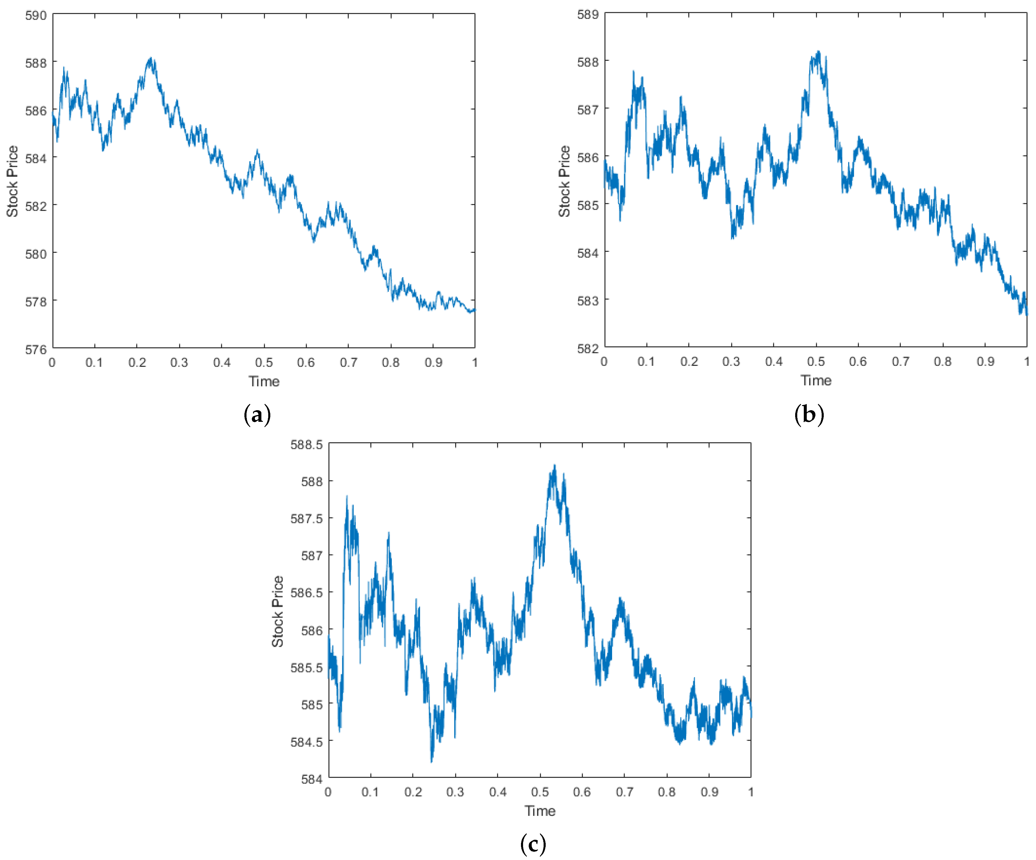
As seen in the previous section, the midprice is assumed to satisfy the SDE, driven by a GCHP, with the approximation achieved using the law of large numbers and the functional central limit theorem. To this definition, we will add the permanent price impact that the agent’s trading action has on the midprice, as seen in Equation (4):

$$d{S}_t^{\nu }=-\left[a^{*}\frac{\lambda }{1-\mu }\left(h\left({\nu }_t\right)\right)\right]dt+\sigma d{W}_t,S_0^{\nu }=S$$

(4)

where $W={\left(W_t\right)}_{\{0\le t\le T\}}$ is a standard Brownian motion, $h,and{\mathbb{R}}_{+}\to {\mathbb{R}}_{+}$ denotes the permanent price impact. The permanent price impact has a negative impact because the agent applies pressure to move the price downward.

Immediately, the midprice and the execution price are presented in Equations (5) and (6):

$$S_t^{\nu }\approx S_0^{\nu }-\left[a^{*}\frac{\lambda }{1-\mu }\left(h\left({\nu }_t\right)\right)\right]t+\sigma W_t,$$

(5)

$${\widehat{S}}_t^{\nu }=S_t^{\nu }-f\left({\nu }_t\right),{\widehat{S}}_0^{\nu }=\widehat{S}$$

(6)

where $f:{\mathbb{R}}_{+}\to {\mathbb{R}}_{+}$ denotes the temporary price impact. The temporary price impact has a negative impact because the agent applies pressure to move the price downward.

To conclude the description of the model, the agent’s cash process $X_t^{\nu }$, which satisfies the SDE in Equation (7):

$$d{X}_t^{\nu }={\widehat{S}}_t^{\nu }{\nu }_{t}dt,X_0^{\nu }=x$$

(7)

and the expected revenue from the sale is as shown in Equation (8):

$$R^{\nu }=\mathbb{E}\left[X_T^{\nu }\right]=\mathbb{E}\left[{\int }_0^T{\widehat{S}}_t{\nu }_{t}dt\right]$$

(8)

The agent’s value function to optimize would involve the terminal cash process $X_T^{\nu }$, the terminal execution $Q_T^{\nu }{S}_T^{\nu }$, and would also incorporate two penalties: a running inventory penalty $\varphi$ and a terminal liquidation penalty $\alpha$, as seen in Equation (10).

$$H^{\nu }(t,x,S,q)={\mathbb{E}}_{t,x,S,q}\left[X_T^{\nu }+Q_T^{\nu }(S_T^{\nu }-\alpha Q_T^{\nu })-\varphi {\int }_t^T{\left(Q_u^{\nu }\right)}^{2}du\right]$$

(9)

$$H(t,x,S,q)=\underset{\mathit{\nu }\in A}{sup}{H}^{\nu }(t,x,S,q)$$

(10)

Applying the theorem of the dynamic programming principle for diffusions (Cartea et al. 2015) to the value function in Equation (10), we obtain the dynamic programming equation (DPE) or HJB equation presented in Equation (11)

$$\begin{array}{cc}\hfill & {\partial }_{t}H+\frac{1}{2}{\sigma }^2{\partial }_{SS}H-\varphi q^2\hfill \\ \hfill & +\underset{\nu }{sup}\{-\nu {\partial }_{q}H-\left(a^{*}\frac{\lambda }{1-\mu }\left(h\left(\nu \right)\right)\right){\partial }_{S}H+\nu (S-f\left(\nu \right)){\partial }_{x}H\}=0\hfill \end{array}$$

(11)

where $\left(a^{*}\frac{\lambda }{1-\mu }\left(h\left(\nu \right)\right)\right){\partial }_{S}H+\frac{1}{2}{\sigma }^2{\partial }_{SS}H$ is the infinitesimal generator of the process $S_t$, as stated in Equation (12).

$$Af\left(s\right)=\left(a^{*}\frac{\lambda }{1-\mu }\right)\frac{\partial f}{\partial s}+\left(\frac{{\sigma }^2}{2}\right)\frac{\partial f^2}{\partial s^2}.$$

(12)

The terminal condition $H(T,x,S,q)=x+Sq-\alpha q^2$ is determined as the inventory q assets are sold in T and it is also penalized in the proportion $\alpha$.The structure of the functions of temporary and permanent impact have not been defined yet. This process can be simplified by letting them be linear with the trading rate. We can write $h\left(\nu \right)=b\nu$ and $f\left(\nu \right)=k\nu$ for $k,b\ge 0$ finite constants. Maximizing by $\nu$, we obtain the following equation, to later solve for $\nu$, and obtain Equation (14).

$$-{\partial }_{q}H-a^{*}\frac{\lambda }{1-\mu }b{\partial }_{S}H+(S-2\nu k){\partial }_{x}H=0$$

(13)

$${\nu }_t^{*}=\frac{1}{2k}\left(\frac{S{\partial }_x-a^{*}\frac{\lambda }{1-\mu }b{\partial }_S-{\partial }_q}{{\partial }_{x}H}\right)H$$

(14)

where ${\nu }^{*}$ is the optimal trading rate, the speed at which the agent is liquidating shares. Upon substituting back into the HJB Equation (11), the value function H is then used to solve the non-linear partial differential equation (PDE).

$${\partial }_{t}H+\frac{1}{2}{\sigma }^2{\partial }_{SS}H-\varphi q^2+\frac{1}{4k}\frac{{\left[\left(S{\partial }_x-a^{*}\frac{\lambda }{1-\mu }b{\partial }_S-{\partial }_q\right)H\right]}^2}{{\partial }_{x}H}=0$$

(15)

To propose an ansatz to solve this equation, we can take a look at the terminal condition and propose a change based on that structure. It is also important to remark that the h function will not be made to depend on the cash process, but H depends on it linearly. The ansatz is shown in Equation (16)

$$H(t,x,S,q)=x+Sq+h(t,S,q)$$

(16)

To match it with the previous terminal condition, our new function h has the terminal condition $h(T,S,q)=-\alpha q^2$. Furthermore, we can write each partial of H in terms of h:

$$\begin{array}{cc}\hfill & {\partial }_{t}H={\partial }_{t}h;{\partial }_{S}H=q+{\partial }_{S}h;{\partial }_{SS}H={\partial }_{SS}h;\hfill \\ \hfill & {\partial }_{X}H=1;{\partial }_{q}H=S+{\partial }_{q}h.\hfill \end{array}$$

(17)

Now we rewrite Equation (15) in terms of h in Equation (18)

$${\partial }_{t}h+\frac{1}{2}{\sigma }^2{\partial }_{SS}h-\varphi q^2+\frac{1}{4k}{\left[a^{*}\frac{\lambda }{1-\mu }b(q+{\partial }_{S}h)+{\partial }_{q}h\right]}^2=0$$

(18)

As suggested in Cartea et al. (2015), we assume the PDE in Equation (18) to be independent of S, because, among other reasons, in the terminal condition h is concerned only with the terminal liquidation penalty. This means that ${\partial }_{S}h(t,S,q)=0$, and also ${\partial }_{SS}h(t,S,q)=0$. With this change, the Equation (18) becomes Equation (19).

$${\partial }_{t}h(t,q)-\varphi q^2+\frac{1}{4k}{\left[a^{*}\frac{\lambda }{1-\mu }bq+{\partial }_{q}h(t,q)\right]}^2=0$$

(19)

With these changes, ${\nu }_t^{*}$ becomes the following equation:

$${\nu }_t^{*}=-\frac{1}{2k}\left(a^{*}\frac{\lambda }{1-\mu }bq+{\partial }_{q}h(t,q)\right)$$

(20)

Based on the terminal condition, where $h(T,S,q)=-\alpha q^2$, we propose a separation of variables with the following form $h(t,q)=h_2\left(t\right)q^2$, where $h_2\left(t\right)$ satisfies the following partials of h:

$${\partial }_{t}h(t,q)={\partial }_t{h}_2\left(t\right)q^2;{\partial }_{q}h(t,q)=2h_2\left(t\right)q.$$

(21)

Now we rewrite the Equation (19) in terms of $h_2$ in Equation (22), with the terminal condition $h_2\left(T\right)=-\alpha$.

$$\begin{array}{cc}\hfill & 0={\partial }_t{h}_2\left(t\right)q^2-\varphi q^2+\frac{1}{4k}{\left[a^{*}\frac{\lambda }{1-\mu }bq+2h_2\left(t\right)q\right]}^2\hfill \\ \hfill & 0={\partial }_t{h}_2-\varphi +\frac{1}{k}{\left[h_2+\frac{1}{2}{a}^{*}\frac{\lambda }{1-\mu }b\right]}^2\hfill \end{array}$$

(22)

This ODE, in Equation (22), is identifiable as a Riccati-type equation to be integrated. We let $h_2\left(t\right)=-\frac{1}{2}{a}^{*}\frac{\lambda }{1-\mu }b+\chi \left(t\right)$, where ${\partial }_t{h}_2\left(t\right)={\partial }_t\chi \left(t\right)$, so we can solve for $\chi \left(t\right)$ to obtain an answer for $h_2\left(t\right)$. This will transform Equation (22) into Equation (23).

$$0={\partial }_t\chi \left(t\right)-\varphi +\frac{1}{k}\chi {\left(t\right)}^2$$

(23)

It is important to remark upon the terminal condition of $\chi \left(t\right)$ is $\chi \left(T\right)=\frac{1}{2}{a}^{*}\frac{\lambda }{1-\mu }b-\alpha$. Now we can solve this differential equation for $\chi$, using substitution and partial fractions to obtain the integral solution in the equation.

$$\begin{array}{cc}\hfill & {\int }_t^T\frac{{\partial }_t\chi }{k\varphi -{\chi }^2}={\int }_t^T\frac{1}{k}\hfill \\ \hfill & \frac{1}{2\sqrt{k\varphi }}\left[log\left(\frac{\sqrt{k\varphi }+\chi \left(T\right)}{\sqrt{k\varphi }-\chi \left(T\right)}\right)-log\left(\frac{\sqrt{k\varphi }+\chi \left(t\right)}{\sqrt{k\varphi }-\chi \left(t\right)}\right)\right]=\frac{1}{k}(T-t)\hfill \\ \hfill & \frac{(\sqrt{k\varphi }-\chi \left(t\right))}{(\sqrt{k\varphi }+\chi \left(t\right))}=\frac{(\sqrt{k\varphi }-\chi \left(T\right))}{(\sqrt{k\varphi }+\chi \left(T\right))}{e}^{2\sqrt{\frac{\varphi }{k}}(T-t)}\hfill \end{array}$$

(24)

From the last equation, we have to solve for $\chi \left(t\right)$. Recall that every part of the right side is a constant, including the terminal condition $\chi \left(T\right)$. Equation (25) expresses an easy way to solve for x.

$$\begin{array}{cc}\hfill & \frac{a-x}{a+x}=c\hfill \\ \hfill & a-x=ca+cx\hfill \\ \hfill & x=a\left(\frac{1-c}{1+c}\right)\hfill \end{array}$$

(25)

To express the final results more easily, we define $\zeta$ a constant composed of the following constants.

$$\zeta =\frac{\alpha -\frac{1}{2}{a}^{*}\frac{\lambda }{1-\mu }b+\sqrt{k\varphi }}{\alpha -\frac{1}{2}{a}^{*}\frac{\lambda }{1-\mu }b-\sqrt{k\varphi }}$$

(26)

$$\chi \left(t\right)=\sqrt{k\varphi }\left(\frac{1+\zeta e^{2\sqrt{\frac{\varphi }{k}}(T-t)}}{1-\zeta e^{2\sqrt{\frac{\varphi }{k}}(T-t)}}\right)$$

(27)

Now the solution of the DPE is fully determined. We can go back to the solution of $h_2\left(t\right)$ in Equation (28) and of $h(t,q)$ in Equation (29).

$$h_2\left(t\right)=-\frac{1}{2}{a}^{*}\frac{\lambda }{1-\mu }b+\sqrt{k\varphi }\left(\frac{1+\zeta e^{2\sqrt{\frac{\varphi }{k}}(T-t)}}{1-\zeta e^{2\sqrt{\frac{\varphi }{k}}(T-t)}}\right)$$

(28)

$$h(t,q)=\left[-\frac{1}{2}{a}^{*}\frac{\lambda }{1-\mu }b+\sqrt{k\varphi }\left(\frac{1+\zeta e^{2\sqrt{\frac{\varphi }{k}}(T-t)}}{1-\zeta e^{2\sqrt{\frac{\varphi }{k}}(T-t)}}\right)\right]q^2$$

(29)

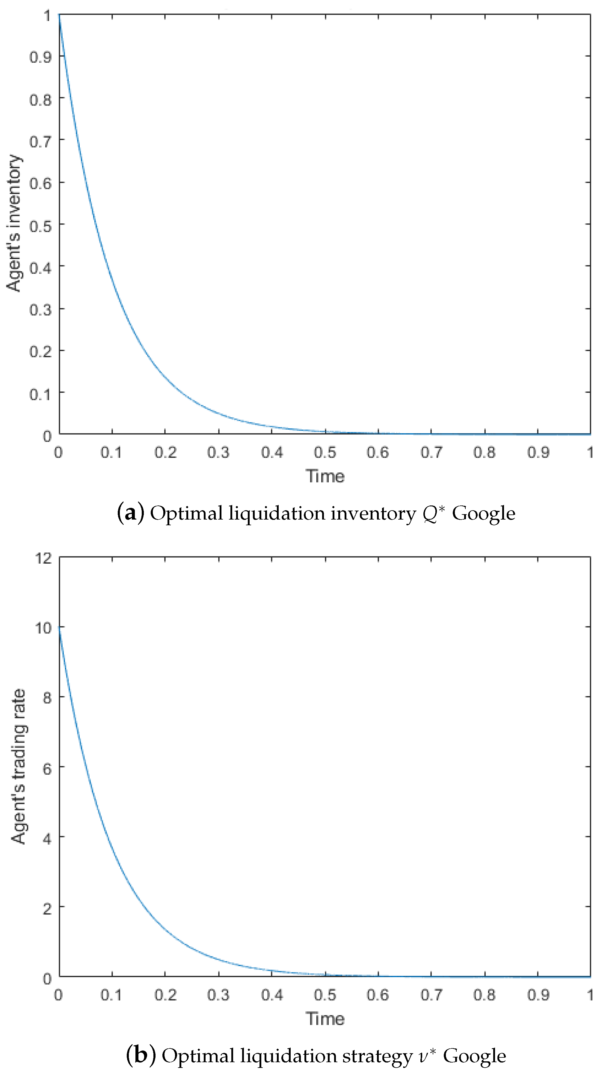
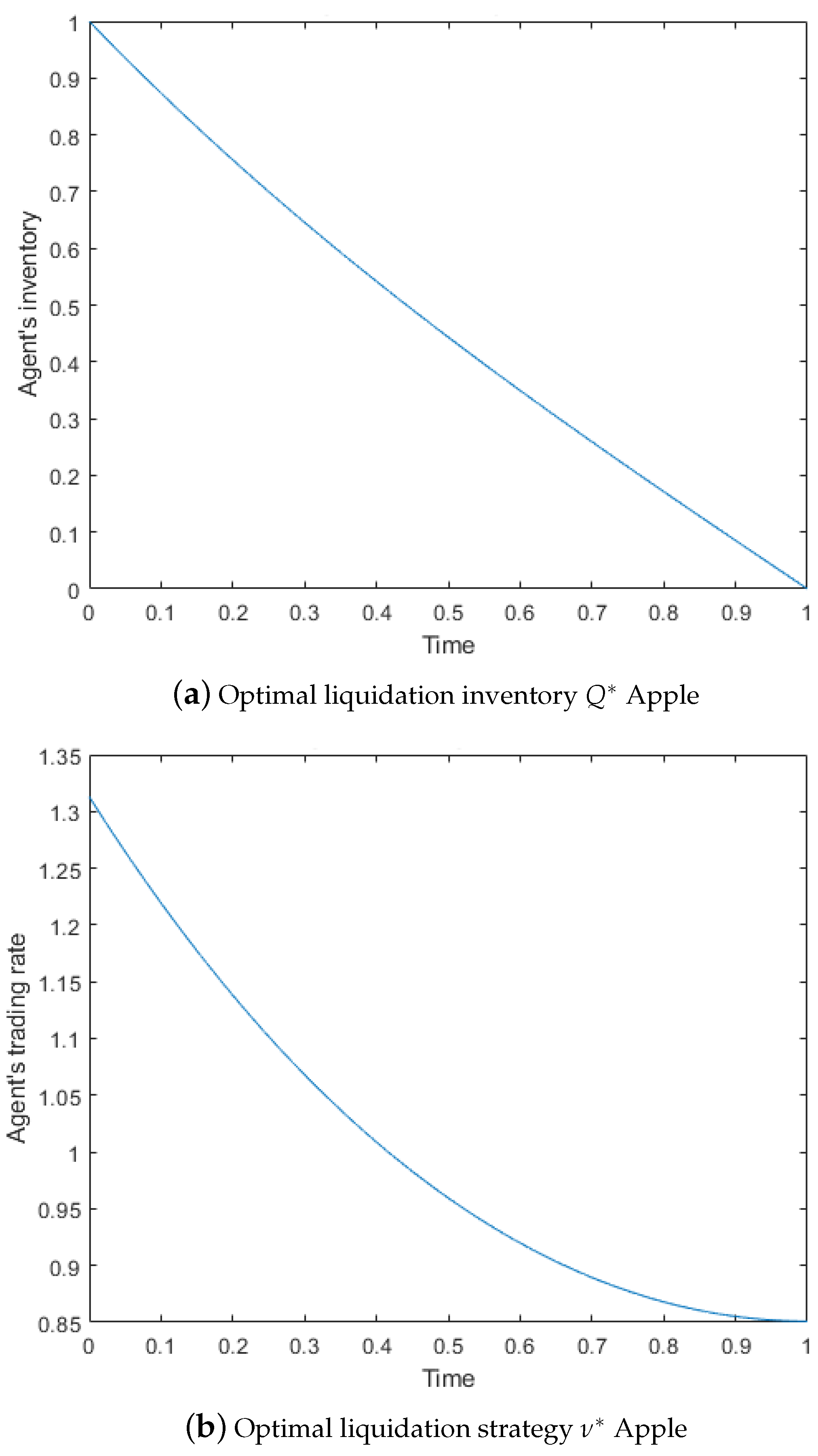
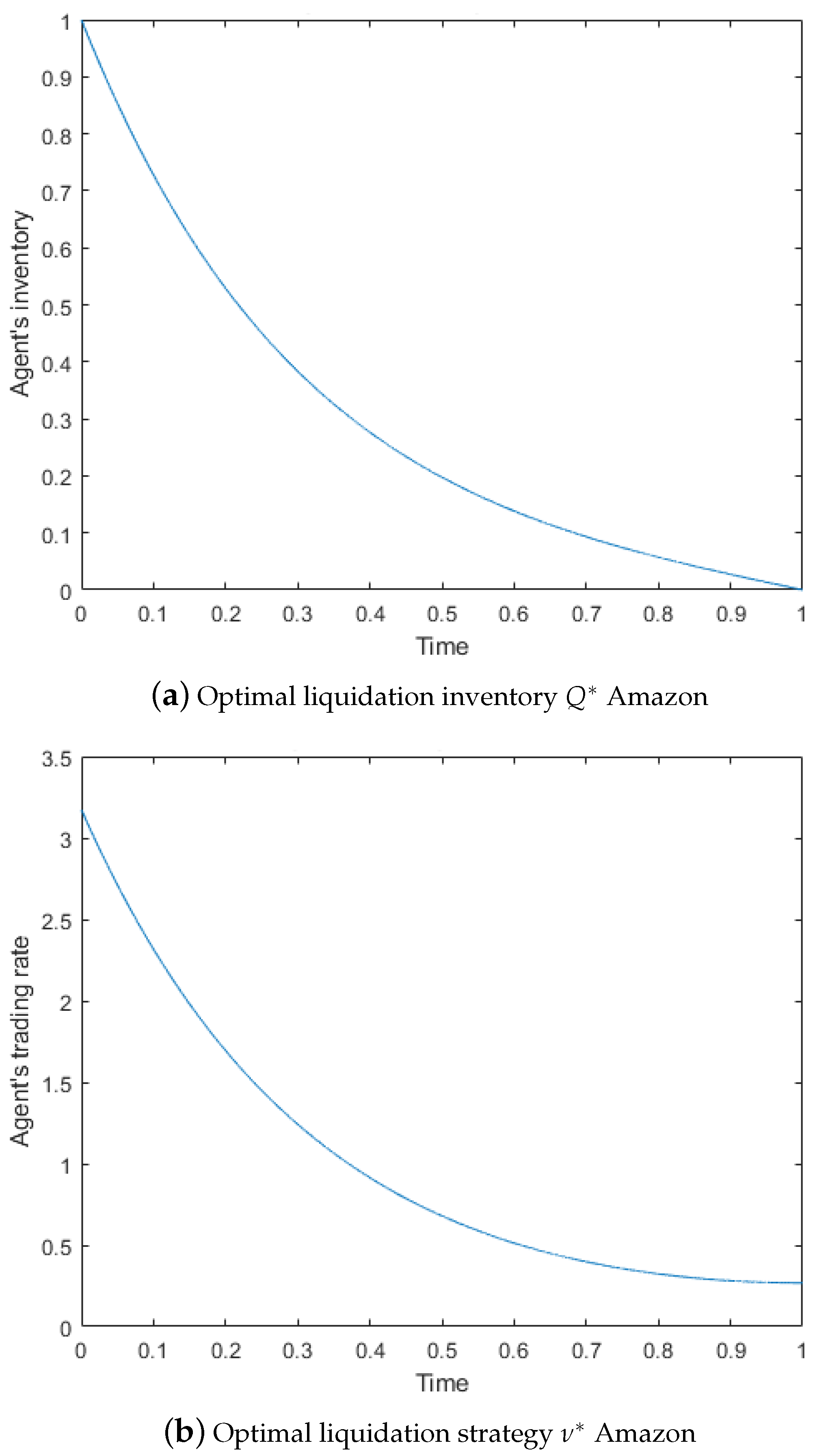
The optimal speed ${\nu }_t^{*}$ can thus be expressed as in Equation (30), and as we can see, the optimal speed turns out to be proportional to $Q^{{\nu }_t^{*}}$, the investor’s current inventory level.

$$\begin{array}{cc}\hfill & {\nu }_t^{*}=-\frac{1}{2k}\left(a^{*}\frac{\lambda }{1-\mu }bq+2q\left[-\frac{1}{2}{a}^{*}\frac{\lambda }{1-\mu }b+\sqrt{k\varphi }\left(\frac{1+\zeta e^{2\sqrt{\frac{\varphi }{k}}(T-t)}}{1-\zeta e^{2\sqrt{\frac{\varphi }{k}}(T-t)}}\right)\right]\right)\hfill \\ \hfill & {\nu }_t^{*}=-\frac{1}{k}\sqrt{k\varphi }\left(\frac{1+\zeta e^{2\sqrt{\frac{\varphi }{k}}(T-t)}}{1-\zeta e^{2\sqrt{\frac{\varphi }{k}}(T-t)}}\right)q\hfill \\ \hfill & {\nu }_t^{*}=\sqrt{\frac{\varphi }{k}}\left(\frac{\zeta e^{\sqrt{\frac{\varphi }{k}}(T-t)}+e^{-\sqrt{\frac{\varphi }{k}}(T-t)}}{\zeta e^{\sqrt{\frac{\varphi }{k}}(T-t)}-e^{-\sqrt{\frac{\varphi }{k}}(T-t)}}\right)Q_t^{{\nu }^{*}}\hfill \end{array}$$

(30)

To obtain the agent’s optimal inventory, $Q_t^{{\nu }^{*}}$, recall the following definitions:

$$\begin{array}{cc}\hfill & d{Q}_t^{\nu }=-{\nu }_{t}dt;d{Q}_t^{\nu }=\frac{1}{k}\sqrt{k\varphi }\left(\frac{1+\zeta e^{2\sqrt{\frac{\varphi }{k}}(T-t)}}{1-\zeta e^{2\sqrt{\frac{\varphi }{k}}(T-t)}}\right)Q_t^{\nu }dt\hfill \\ \hfill & d{Q}_t^{\nu }=\frac{\chi \left(t\right)}{k}{Q}_t^{\nu }dtd\left(log\left(Q_t^{\nu }\right)\right)=\frac{\chi \left(t\right)}{k}dt\hfill \\ \hfill & log\left(Q_t^{\nu }\right)+C={\int }_0^t\frac{\chi \left(s\right)}{k}ds{Q}_t^{\nu }=C_2{e}^{{\int }_0^t\frac{\chi \left(s\right)}{k}ds}\hfill \end{array}$$

(31)

This constant $C_2$ can be calibrated with the initial value ($t=0$) of the inventory $\mathfrak{N}$. Next, let us solve the integral in $Q_t^{\nu }$

$$\begin{array}{cc}\hfill & {\int }_0^t\frac{\chi \left(s\right)}{k}ds=\frac{1}{k}{\int }_0^t\sqrt{k\varphi }\left(\frac{1+\zeta e^{2\sqrt{\frac{\varphi }{k}}(T-s)}}{1-\zeta e^{2\sqrt{\frac{\varphi }{k}}(T-s)}}\right)ds\hfill \\ \hfill & =\sqrt{\frac{\varphi }{k}}{\int }_0^t\frac{1}{1-\zeta e^{2\sqrt{\frac{\varphi }{k}}(T-s)}}ds+\sqrt{\frac{\varphi }{k}}{\int }_0^t\frac{\zeta e^{2\sqrt{\frac{\varphi }{k}}(T-s)}}{1-\zeta e^{2\sqrt{\frac{\varphi }{k}}(T-s)}}ds\hfill \\ \hfill & =\frac{1}{2}\left[log(e^{-2\sqrt{\frac{\varphi }{k}}(T-s)}-\zeta )+log(1-\zeta e^{2\sqrt{\frac{\varphi }{k}}(T-s)})\right]{|}_0^t\hfill \\ \hfill & =log\left(\frac{\zeta e^{\sqrt{\frac{\varphi }{k}}(T-t)}-e^{-\sqrt{\frac{\varphi }{k}}(T-t)}}{\zeta e^{\sqrt{\frac{\varphi }{k}}T}-e^{-\sqrt{\frac{\varphi }{k}}T}}\right)\hfill \end{array}$$

(32)

Finally, we obtain the optimal agent’s inventory in Equation (33) and the optimal trading rate in Equation (34) is solved. It is worth mentioning that this solution is very similar to the results presented in Cartea et al. (2015) but this time the solution includes the parameters of the arrival rate and the counting process introduced in the Hawkes process.

$$Q_t^{{\nu }^{*}}=\left(\frac{\zeta e^{\sqrt{\frac{\varphi }{k}}(T-t)}-e^{-\sqrt{\frac{\varphi }{k}}(T-t)}}{\zeta e^{\sqrt{\frac{\varphi }{k}}T}-e^{-\sqrt{\frac{\varphi }{k}}T}}\right)\mathfrak{N}$$

(33)

$${\nu }_t^{*}=\sqrt{\frac{\varphi }{k}}\left(\frac{\zeta e^{\sqrt{\frac{\varphi }{k}}(T-t)}+e^{-\sqrt{\frac{\varphi }{k}}(T-t)}}{\zeta e^{\sqrt{\frac{\varphi }{k}}T}-e^{-\sqrt{\frac{\varphi }{k}}T}}\right)\mathfrak{N}$$

(34)

${\nu }_t^{*}$ expresses the optimal strategy for every t. The value of $\zeta$ contains, among other factors, the terminal liquidation inventory $\alpha$, the compound Hawkes process parameters $\lambda$ and $\mu$, and the coefficient of the permanent price impact b. The ratio between the running inventory penalty $\varphi$ and the coefficient of the temporal price impact k weights the optimal strategy.

In Section 6.3 we present numerical results using the observed price data for Apple, Amazon, and Google on 21 June 2012 (LOBster data LOBster 2012) and the parameter calibration of parameters $a\ast$ and $\frac{\lambda }{1-\mu }$ from Swishchuk and Huffman (2020) for the GCHP2SDO. We calculated the optimal liquidation strategy for an agent’s trading rate, ${\nu }^{*}$, and the optimal depth ${\delta }^{*,\pm }$. In Section 6.3, the results are drawn to show the behavior of the optimal strategy throughout the time available. The parameters used for k, b, $\varphi$, $\alpha$, $\mathfrak{N}$, T, $\kappa$, and ${\lambda }^{\pm }$ are shown in the tables of each stock, according to the model and the asset drawn.

4. Optimal Acquisition Problem

In this problem, the agent has the target to acquire $\mathfrak{N}$ shares over a trading horizon of T. The key stochastic processes are the same as those described in the previous section. The agent’s inventory starts at $Q_0^{\nu }=0$. The terminal inventory penalty parameter $\alpha$ includes the cost of walking the book at time T.

The midprice and the execution price are similar to the price presented in Equations (5) and (6), with the difference in the signs of the influence of the temporary and permanent impacts. Because the agent’s buy trade exercises an upward pressure, this is displayed in Equations (35) and (36):

$$S_t^{\nu }\approx S_0^{\nu }+\left[a^{*}\frac{\lambda }{1-\mu }\left(h\left({\nu }_t\right)\right)\right]t+\sigma W_t,$$

(35)

$${\widehat{S}}_t^{\nu }=S_t^{\nu }+f\left({\nu }_t\right),{\widehat{S}}_0^{\nu }=\widehat{S}$$

(36)

The agent’s expected costs from strategy ${\nu }_t$ are integrated by means of the terminal cash, the terminal execution, and terminal penalty, described in Equation (37).

$$E{C}^{\nu }=\mathbb{E}\left[{\int }_t^T{\widehat{S}}_u^{\nu }{\nu }_{u}du+\left(\mathfrak{N}-Q_T^{\nu }\right)S_T+\alpha {\left(\mathfrak{N}-Q_T^{\nu }\right)}^2\right]$$

(37)

Let us define a new stochastic process, $Y{\nu }_t$, that denotes the remaining shares to be purchased between t and the end of the period. This is defined in Equation (38), where

$$Y^{\nu }={\left(Y_t^{\nu }\right)}_{\{0\le t\le T\}}$$

(38)

is the agent’s remaining shares.

$$Y_t^{\nu }=\mathfrak{N}-Q_t^{\nu },sothatd{Y}_t^{\nu }=-{\nu }_{t}dt$$

The agent’s value function to optimize would involve the agent’s expected cost, so we need to minimize or calculate the infimum of the cash paid to acquire the shares, as shown in Equation (40).

$$H^{\nu }(t,S,y)={\mathbb{E}}_{t,S,y}\left[{\int }_t^T{\widehat{S}}_u^{\nu }{\nu }_{u}du+Y_T^{\nu }{S}_T+\alpha {\left(Y_T^{\nu }\right)}^2\right]$$

(39)

$$H(t,S,y)=\underset{\mathit{\nu }\in A}{inf}{H}^{\nu }(t,S,y)$$

(40)

Applying the theorem dynamic programming principle for diffusions (Cartea et al. 2015) to the value function in Equation (40), we obtain the dynamic programming equation (DPE) or HJB equation in (41):

$$\begin{array}{cc}\hfill & {\partial }_{t}H+\frac{1}{2}{\sigma }^2{\partial }_{SS}H\hfill \\ \hfill & +\underset{\nu }{inf}\{-\nu {\partial }_{y}H+\left(a^{*}\frac{\lambda }{1-\mu }\left(h\left(\nu \right)\right)\right){\partial }_{S}H+\nu \left({\widehat{S}}_t^{\nu }\right)\}=0\hfill \end{array}$$

(41)

where $\left(a^{*}\frac{\lambda }{1-\mu }\left(h\left(\nu \right)\right)\right){\partial }_{S}H+\frac{1}{2}{\sigma }^2{\partial }_{SS}H$ is the infinitesimal generator of the process $S_t$ as stated in Equation (12).

The terminal condition $H(T,S,y)=yS+\alpha y^2$ is determined as the remaining inventory y assets are purchased in T and also it is penalized in the proportion $\alpha$. The structure of the function of temporary and permanent impacts has not been defined yet. As in the previous section, this will be simplified by allowing them to be linear with the trading rate. We can write $h\left(\nu \right)=b\nu$ and $f\left(\nu \right)=k\nu$ for $k,b\ge 0$, which are finite constants. Minimizing by $\nu$, we obtain the following equation to later solve for $\nu$ and we obtain Equation (43).

$$-{\partial }_{y}H+a^{*}\frac{\lambda }{1-\mu }b{\partial }_{S}H+(S+2\nu k)=0$$

(42)

$${\nu }^{*}=\frac{1}{2k}\left({\partial }_{y}H-S-a^{*}\frac{\lambda }{1-\mu }b{\partial }_{S}H\right)$$

(43)

where ${\nu }^{*}$ is the optimal trading rate, the speed at which the agent is acquiring shares. Upon substituting back into the HJB Equation (41), the value function H then solves the non-linear partial differential equation (PDE).

$${\partial }_{t}H+\frac{1}{2}{\sigma }^2{\partial }_{SS}H-\frac{1}{4k}{\left({\partial }_{y}H-S-a^{*}\frac{\lambda }{1-\mu }b{\partial }_{S}H\right)}^2=0$$

(44)

By observing the terminal condition and the way in which y and S enter into the DPE, we propose a quadratic function in y to use as the ansatz to solve this equation. The ansatz is shown in Equation (45)

$$H(t,S,y)=yS+h_0\left(t\right)+h_1\left(t\right)y+h_2\left(t\right)y^2$$

(45)

where $h_0\left(t\right)$, $h_1\left(t\right)$, and $h_2\left(t\right)$ are yet to be determined according to the terminal condition $H(T,S,y)=yS+\alpha y^2$; then, $h_2\left(T\right)=\alpha$ and $h_1\left(T\right)=h_0\left(T\right)=0$. To match them with the previous terminal condition, our new functions $h_0$, $h_1$ and $h_2$ can express each partial of H in terms of the new functions:

$$\begin{array}{cc}\hfill & {\partial }_{t}H={\partial }_t{h}_0+y{\partial }_t{h}_1+y^2{\partial }_t{h}_2;\hfill \\ \hfill & {\partial }_{S}H=y;{\partial }_{SS}H=0;\hfill \\ \hfill & {\partial }_{y}H=S+h_1+2h_{2}y.\hfill \end{array}$$

(46)

Now we rewrite the Equation (44) in terms of $h_0$, $h_1$, and $h_2$ in Equation (47)

$${\partial }_t{h}_0+y{\partial }_t{h}_1+y^2{\partial }_t{h}_2-\frac{1}{4k}{\left[h_1+y\left(2h_2-a^{*}\frac{\lambda }{1-\mu }b\right)\right]}^2=0$$

(47)

It is worth mentioning that with this new structure, the second derivative of H becomes zero and this causes the effect of $\sigma$ to disappear. Now, with help of the boundary conditions, we are able to solve for $h_0$, $h_1$, and $h_2$. Let us order the equation as follows:

$$\begin{array}{c}\hfill \left\{{\partial }_t{h}_2-\frac{1}{4k}{\left(2h_2-a^{*}\frac{\lambda }{1-\mu }b\right)}^2\right\}{y}^2+\left\{{\partial }_t{h}_1-\frac{1}{2k}{h}_1\left(2h_2-a^{*}\frac{\lambda }{1-\mu }b\right)\right\}y\\ \hfill +\left\{{\partial }_t{h}_0-\frac{1}{4k}{h}_1^2\right\}=0\end{array}$$

(48)

Let us write $\frac{1}{2k}\left(2h_2-a^{*}\frac{\lambda }{1-\mu }b\right)=f\left(t\right)$ and then, using the second term in Equation (48), the coefficient of y, we obtain the following:

$$\begin{array}{cc}\hfill & {\partial }_t{h}_1-\frac{1}{2k}{h}_1\left(2h_2-a^{*}\frac{\lambda }{1-\mu }b\right)=0\hfill \\ \hfill & \frac{{\partial }_t{h}_1}{h_1}=f\left(t\right)\hfill \\ \hfill & dlog\left(h_1\right)=f\left(t\right)\hfill \\ \hfill & log\left(h_1\right)+c_1=\int f\left(s\right)ds\hfill \\ \hfill & h_1=c_1^{\prime }{e}^{\int f\left(s\right)ds},asfor{h}_1\left(T\right)=0\hfill \\ \hfill & 0=c_1^{\prime }{e}^{{\int }_0^{T}f\left(s\right)ds},\iff c_1^{\prime }=0\Rightarrow h_1\left(t\right)=0\hfill \end{array}$$

(49)

From the third term in Equation (48), the independent coefficient, we obtain the following:

$$\begin{array}{cc}\hfill & as{h}_1=0,\Rightarrow {\partial }_t{h}_0=0\hfill \\ \hfill & \Rightarrow h_0=c_2,h_0\left(T\right)=0=c_2\hfill \\ \hfill & \iff c_2=0\Rightarrow h_0\left(t\right)=0\hfill \end{array}$$

(50)

Finally, we can solve $h_2$ from the first term in Equation (48), the coefficient of $y^2$.

$$\begin{array}{cc}\hfill & ϵ=a^{*}\frac{\lambda }{1-\mu }b\hfill \\ \hfill & {\partial }_t{h}_2-\frac{1}{4k}{\left(2h_2-ϵ\right)}^2=0\hfill \end{array}$$

(51)

Rewriting this in the form of a first-order separable ODE:

$$\begin{array}{cc}\hfill & \int \frac{4k}{{\left(2h_2-ϵ\right)}^2}{\partial }_t{h}_2=\int 1dt\hfill \\ \hfill & \frac{-2k}{2h_2-ϵ}=t+c_3\hfill \\ \hfill & h_2=\left[\frac{-2k}{t+c_3}+ϵ\right]\frac{1}{2}\hfill \end{array}$$

(52)

Matching $h_2\left(T\right)$ from Equation (52) and the terminal condition $h_2\left(T\right)=\alpha$, we can define the value of $c_3$ as follows:

$$\begin{array}{cc}\hfill & \alpha =\frac{1}{2(T+c_3)}\left[-2k+ϵT+ϵc_3\right]\hfill \\ \hfill & c_3=\frac{-2k}{2\alpha -ϵ}-T\hfill \end{array}$$

(53)

Now, the solution is fully determined as $H(t,S,y)=yS+h_2\left(t\right)y^2$. With these changes, ${\nu }_t^{*}$ becomes Equation (54).

$${\nu }_t^{*}=\frac{1}{2k}\left(2h_2\left(t\right)-ϵ\right)Y_t^{{\nu }^{*}}$$

(54)

From the derivative defined as $d{Y}_t^{\nu }=-{\nu }_{t}dt$ from Equation (38), we can obtain the optimal agent’s remaining shares $Y_t^{{\nu }^{*}}$ as follows:

$$\begin{array}{cc}\hfill & d{Y}_t^{\nu }=-\frac{1}{2k}\left(2h_2\left(t\right)-ϵ\right)Y_t^{\nu }dt\hfill \\ \hfill & \frac{d{Y}_t^{\nu }}{Y_t^{\nu }}=-\frac{1}{2k}\left(2h_2\left(t\right)-ϵ\right)dt\int d\left(log\left(Y_t^{\nu }\right)\right)=\int -\frac{1}{2k}\left(2h_2\left(u\right)-ϵ\right)du\hfill \\ \hfill & log\left(Y_t^{\nu }\right)={\int }_0^t-\frac{1}{2k}\left(\frac{-2k}{u+c_3}+ϵ-ϵ\right)dulog\left(Y_t^{\nu }\right)={\int }_0^t\frac{1}{u+c_3}du\hfill \\ \hfill & log\left(Y_t^{\nu }\right)=log\left(\frac{t}{c_3}+1\right)+c_4{Y}_t^{\nu }=\left(1+\frac{t}{c_3}\right)e^{c_4}\hfill \end{array}$$

(55)

From our initial assumptions, where $Y_0^{\nu }=\mathfrak{N}$, we can conclude that $e^{c_4}=\mathfrak{N}$. Furthermore, from $Y_t^{\nu }=\mathfrak{N}-Q_t^{\nu }$ we can obtain the optimal agent’s inventory $Q_t^{{\nu }^{*}}$ and we obtain it as follows:

$$\begin{array}{cc}\hfill & Q_t^{\nu }=\mathfrak{N}\left(1-1-\frac{t}{c_3}\right)Q_t^{\nu }=-\mathfrak{N}\frac{t}{c_3}\hfill \\ \hfill & Q_t^{\nu }=\mathfrak{N}\frac{t(2\alpha -ϵ)}{2k+2\alpha T-ϵT}{Q}_t^{\nu }=\mathfrak{N}t\left(\frac{1-\frac{ϵ}{2\alpha }}{\frac{k}{\alpha }+\left(1-\frac{ϵ}{2\alpha }\right)T}\right)\hfill \end{array}$$

(56)

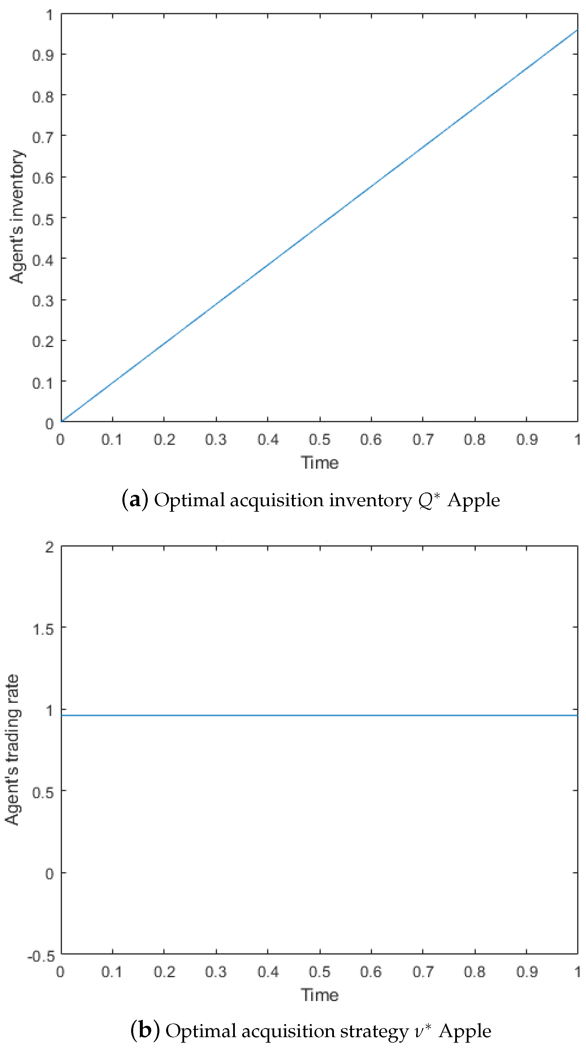
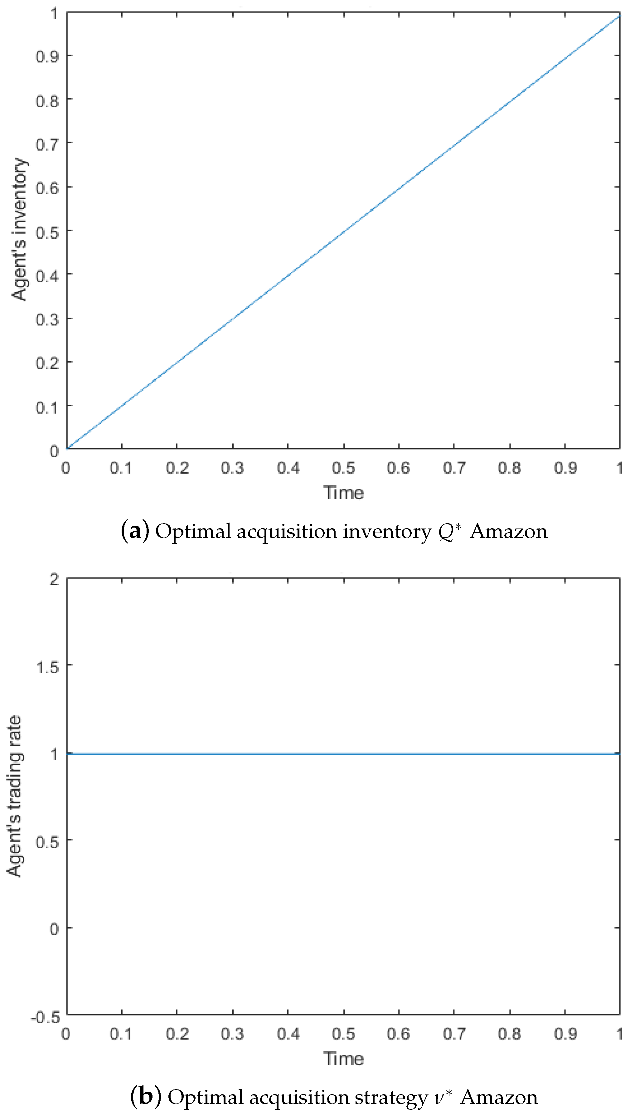
Finally, we can obtain the optimal speed for acquisition in (57)

$${\nu }_t^{*}=\mathfrak{N}\left(\frac{1-\frac{ϵ}{2\alpha }}{\frac{k}{\alpha }+\left(1-\frac{ϵ}{2\alpha }\right)T}\right)$$

(57)

${\nu }_t^{*}$ expresses the optimal strategy for every t. The value of $ϵ$ contains the compound Hawkes process parameters $\lambda$, $\mu$, and the coefficient of the permanent price impact b. The ratio between the coefficient of the temporal price impact k and the terminal liquidation inventory $\alpha$ is known as the relative price impact at the terminal date and, in general, $\alpha \gg k$; then $\frac{k}{\alpha }<1$.

In Section 6.4 we present numerical results using the price data observed for Apple, Amazon, and Google on 21 June 2012 (LOBster data) LOBster (2012) and the parameter calibration of parameters $a\ast$ and $\frac{\lambda }{1-\mu }$ from Swishchuk and Huffman (2020) for the GCHP2SDO. We calculated the optimal acquisition strategy for the agent’s trading rate, ${\nu }^{*}$, and the optimal depth ${\delta }^{*,\pm }$. In Section 6.4, the results are drawn to show the behavior of the optimal strategy throughout the time available. The parameters used for k, b, $\varphi$, $\alpha$, $\mathfrak{N}$, T, $\kappa$, and ${\lambda }^{\pm }$ are shown in the tables of each stock, according to the model and the asset drawn.

5. Optimal Market-Making Problem

The market-making problem models how a market maker (MM) maximizes terminal wealth by trading in and out of positions using limit orders (LOs). The MM provides liquidity to the limit order book (LOB) by posting buy and sell LOs, and the control variable is the depth $\delta$, which is measured based on the midprice, at which these LOs are posted. The key stochastic processes for this model are:

• $S={\left(S_t\right)}_{0\le t\le T}$, denotes the midprice, assumed to satisfy the SDE driven by a GCHP, as seen in Equation (4), with $S_t^{\pm }=S_0\pm \left[a^{*}\frac{\lambda }{1-\mu }\right]t+\sigma W_t$, $\sigma >0$ and $W={\left(W_t\right)}_{0\le t\le T}$ is a standard Brownian motion, $S_t^{+}$ is the price for the acquisition side, and $S_t^{-}$ is the price for the liquidation side;
• ${\delta }^{\pm }={\left({\delta }_t^{\pm }\right)}_{0\le t\le T}$ denote the depth at which the agent posts LOs; sell LOs are posted at a price of $S_t^{-}+{\delta }_t^{+}$, and buy LOs at a price of $S_t^{+}-{\delta }_t^{-}$;
• $M^{\pm }={\left(M_t^{\pm }\right)}_{0\le t\le T}$ denote the counting processes corresponding to the arrival of other participants’ buy $(+)$ and sell $(-)$ market orders (MOs), which arrive at Poisson times with intensities ${\lambda }^{\pm }$;
• $N^{\delta ,\pm }={(N_t^{\delta ,\pm })}_{0\le t\le T}$ denote the controlled counting processes for the agent’s filled sell $(+)$ and buy $(-)$ LOs;
• $X^{\delta }={\left(X_t^{\delta }\right)}_{0\le t\le T}$ denote the MM’s cash process and this satisfies the SDE

  $$d{X}_t^{\delta }=(S_t^{-}+{\delta }_t^{+})d{N}_t^{\delta ,+}-(S_t^{+}-{\delta }_t^{-})d{N}_t^{\delta ,-};$$

  (58)
• $Q^{\delta }={\left(Q_t^{\delta }\right)}_{0\le t\le T}$ denotes the agent’s inventory process and

  $$Q_t^{\delta }=N_t^{\delta ,-}-N_t^{\delta ,+}$$

  (59)

For the counting processes, $N_t^{\delta }$ is not a Poisson process. The intensity of the process $N_t^{\delta }$ is controlled by the agent, because the greater the depth, $\delta$, the lower is the probability of the LO being filled. The probability of the arrival rate of the MO’s other market participants is a constant $\lambda >0$. Modeling the probability of the LO being filled is conditional on the MO arriving, and this is a popular choice in the literature, as in Cartea et al. (2015) (see discussion in Section 5.4), where it is expressed by theprobability $e^{-{\kappa }^{\pm }{\delta }_t^{\pm }}$, where $\kappa$ is a positive constant. Finally, following the Bayes rule, the fill probability would be the product of these two, ${\mathsf{\Lambda }}_t^{\delta ,\pm }={\lambda }^{\pm }{e}^{-{\kappa }_{\pm }{\delta }_t^{\pm }}$.

The market maker seeks the strategy ${\left({\delta }_s^{\pm }\right)}_{0\le s\le T}$ that maximizes cash at the terminal date T. The MM must liquidate their terminal inventory $Q_T$ at time T using MO. Then, the MM adds boundaries to the inventory via $\underset{¯}{q}<0<\overline{q}$, both of which are finite. Thus, the performance criteria are as presented in Equation (60):

$$H^{\delta }(t,x,q,S^{+},S^{-})={\mathbb{E}}_{t,x,q,S^{+},S^{-}}\left[X_T+Q_T^{\delta }(S^{-,{\delta }_T}-\alpha Q_T^{\delta })-\varphi {\int }_t^T{\left(Q_u\right)}^{2}du\right]$$

(60)

where $\alpha \ge 0$ represents the fees charged for taking liquidity at the end of the term and $\varphi \ge 0$ is the running inventory penalty parameter. Thus, the MM’s value function is as shown in Equation (61):

$$H(t,x,q,S^{+},S^{-})=\underset{{\delta }^{\pm }\in A}{sup}{H}^{\delta }(t,x,q,S^{+},S^{-}),$$

(61)

where A is the admissible set of strategies, $\mathcal{F}$-predictable, and bounded from below. Now, let us solve the optimal control problem, applying the theorem of the dynamic programming principle for counting processes (Cartea et al. 2015). As we defined in the key stochastic processes for this model, there exist two different prices for the bid and ask side. Thus, the HJB equation is as shown in Equation (62):

$$\begin{array}{cc}\hfill & 0={\partial }_{t}H+{\sigma }^2{\partial }_{SS}H-a^{*}\frac{\lambda }{1-\mu }{\partial }_{S^{-}}H+a^{*}\frac{\lambda }{1-\mu }{\partial }_{S^{+}}H-\varphi q^2\hfill \\ \hfill & +{\lambda }^{+}\underset{{\delta }^{+}}{sup}\left\{e^{-{\kappa }^{+}{\delta }^{+}}\left(H(t,x+(S^{-}+{\delta }^{+}),q-1,S^{-})-H(t,x,q,S^{+})\right)\right\}\mathrm{𝟙}q>\underset{¯}{q}\hfill \\ \hfill & +{\lambda }^{-}\underset{{\delta }^{-}}{sup}\left\{e^{-{\kappa }^{-}{\delta }^{-}}\left(H(t,x-(S^{+}-{\delta }^{-}),q+1,S^{+})-H(t,x,q,S^{-})\right)\right\}\mathrm{𝟙}q<\overline{q}\hfill \end{array}$$

(62)

where $\left(a^{*}\frac{\lambda }{1-\mu }\right){\partial }_S^{+}H+\frac{1}{2}{\sigma }^2{\partial }_{S^{+}{S}^{+}}H$ is the infinitesimal generator of the process $S_t^{+}$, and likewise for $S_t^{-}$, as stated in Equation (12). In this case, to simplify the analysis, we assume that ${\partial }_{S^{-}{S}^{-}}H={\partial }_{S^{+}{S}^{+}}H$; then it can be written as ${\partial }_{SS}$. $\mathrm{𝟙}$ is the indicator function.

The terminal condition $H(T,x,q,S^{-})=x+q(S^{-}-\alpha q)$ is determined as the market maker, at the end of the time period, will liquidate the terminal inventory at the liquidation price and it is also penalized in the proportion of $\alpha$. Following this terminal condition, we propose an ansatz for H, as shown in Equation (63):

$$H(t,x,q,S^{+},S^{-})=x+q{S}^{-}+h(t,q)$$

(63)

To match this with the previous terminal condition, our new function h has the terminal condition $h(T,q)=-\alpha q^2$. We can also write each partial of H in terms of h:

$$\begin{array}{cc}\hfill & {\partial }_{t}H={\partial }_{t}h(t,q);{\partial }_{S^{-}}H=q;\hfill \\ \hfill & {\partial }_{S^{+}}H=0;{\partial }_{SS}H=0\hfill \end{array}$$

(64)

$$\begin{array}{cc}\hfill & H(t,x-(S^{-}-{\delta }^{+}),q-1,S^{+},S^{-})-H(t,x,q,S^{+},S^{-})={\delta }^{+}+h(t,q-1)-h(t,q)\hfill \\ \hfill & H(t,x-(S^{+}-{\delta }^{-}),q+1,S^{+},S^{-})-H(t,x,q,S^{+},S^{-})=-S^{+}+S^{-}+{\delta }^{-}+h(t,q+1)-h(t,q)\hfill \\ \hfill & -S^{+}+S^{-}+=-2a^{*}\frac{\lambda }{1-\mu }t\hfill \end{array}$$

(65)

Now we can rewrite the Equation (62) in terms of h in Equation (66):

$$\begin{array}{cc}\hfill & \varphi q^2+a^{*}\frac{\lambda }{1-\mu }q={\partial }_{t}h(t,q)\hfill \\ \hfill & +{\lambda }^{+}\underset{{\delta }^{+}}{sup}\left\{e^{-{\kappa }^{+}{\delta }^{+}}\left({\delta }^{+}+h(t,q-1)-h(t,q)\right)\right\}{\mathrm{𝟙}}_{q>\underset{¯}{q}}\hfill \\ \hfill & +{\lambda }^{-}\underset{{\delta }^{-}}{sup}\left\{e^{-{\kappa }^{-}{\delta }^{-}}\left({\delta }^{-}+h(t,q+1)-h(t,q)-2a^{*}\frac{\lambda }{1-\mu }t\right)\right\}{\mathrm{𝟙}}_{q<\overline{q}}\hfill \end{array}$$

(66)

Maximizing by ${\delta }^{+}$ and ${\delta }^{-}$, we obtain the following equation to later solve for ${\delta }^{+}$ and ${\delta }^{-}$ and we obtain Equations (68) and (70).

$$0={\lambda }^{+}[e^{-{\kappa }^{+}{\delta }^{+}}(-{\kappa }^{+})({\delta }^{+}+h(t,q-1)-h(t,q))+e^{-{\kappa }^{+}{\delta }^{+}}],q\ne \underset{¯}{q}$$

(67)

$${\delta }^{+}=\frac{1}{{\kappa }^{+}}-h(t,q-1)+h(t,q),q\ne \underset{¯}{q}$$

(68)

$$0={\lambda }^{-}[e^{-{\kappa }^{-}{\delta }^{-}}(-{\kappa }^{-})({\delta }^{-}+h(t,q+1)-h(t,q)-2a^{*}\frac{\lambda }{1-\mu }t)+e^{-{\kappa }^{-}{\delta }^{-}}],q\ne \overline{q}$$

(69)

$${\delta }^{-}=\frac{1}{{\kappa }^{-}}-h(t,q+1)+h(t,q)+2a^{*}\frac{\lambda }{1-\mu }t,q\ne \overline{q}$$

(70)

Now, the boundary cases are ${\delta }^{+,*}(t,q)=+\infty$ and ${\delta }^{-,*}(t,q)=+\infty$ when $q=\overline{q}$ and $\underset{¯}{q}$, respectively.

With these maximized strategies, we can substitute the optimal controls into the DPE in Equation (66):

$$\begin{array}{cc}\hfill & \varphi q^2+a^{*}\frac{\lambda }{1-\mu }q={\partial }_{t}h(t,q)\hfill \\ \hfill & +\frac{{\lambda }^{+}}{{\kappa }^{+}}{e}^{-{\kappa }^{+}(\frac{1}{{\kappa }^{+}}-h(t,q-1)+h(t,q))}{\mathrm{𝟙}}_{q>\underset{¯}{q}}\hfill \\ \hfill & +\frac{{\lambda }^{-}}{{\kappa }^{-}}{e}^{-{\kappa }^{-}(\frac{1}{{\kappa }^{-}}-h(t,q+1)+h(t,q)+2a^{*}\frac{\lambda }{1-\mu }t)}{\mathrm{𝟙}}_{q<\overline{q}}\hfill \end{array}$$

(71)

To find an analytical solution, we need to match it with the previous terminal condition. We propose to use the following function for $h(t,q)$, where the terminal condition $h(T,q)=-\alpha q^2$ prevails. As was carried out in a previous work (Cartea et al. 2015), we define the fill probabilities to be the same on both sides of the LOB, meaning that $\kappa ={\kappa }^{+}={\kappa }^{-}$, and thus express the suggested ansatz as follows:

$$h(t,q)=\frac{1}{\kappa }log\omega (t,q)$$

(72)

with the terminal condition $\omega (T,q)=e^{-\alpha \kappa q^2}$; then $h(T,q)=\frac{1}{\kappa }log(e^{-\alpha \kappa q^2})=-\alpha q^2$.

Now, we have to match the new ansatz with the previous PDE Equation (71)

$$\begin{array}{cc}\hfill & {\partial }_{t}h(t,q)=\frac{1}{\kappa }{\partial }_t\omega (t,q)\frac{1}{\omega (t,q)};\hfill \\ \hfill & e^{-1}{e}^{log(\frac{\omega (t,q-1)}{\omega (t,q)})}=e^{-1}\frac{\omega (t,q-1)}{\omega (t,q)};\hfill \\ \hfill & and{e}^{-1}{e}^{-2a^{*}\frac{\lambda }{1-\mu }t\kappa }\frac{\omega (t,q+1)}{\omega (t,q)}\hfill \end{array}$$

(73)

Putting all together in Equation (74),

$$\begin{array}{cc}\hfill & (\varphi q^2\kappa +a^{*}\frac{\lambda }{1-\mu }q\kappa )\omega (t,q)={\partial }_t\omega (t,q)+{\lambda }^{+}{e}^{-1}\omega (t,q-1)\hfill \\ \hfill & +{\lambda }^{-}{e}^{-(1+2a^{*}\frac{\lambda }{1-\mu }t\kappa )}\omega (t,q+1)\hfill \end{array}$$

(74)

Let us break the vector $\omega (t,q)$ from $\overline{q}$ to $\underset{¯}{q}$, and let $A\left(t\right)$ denote the $(\overline{q}-\underset{¯}{q}+1)$ square matrix described below.

$$\omega \left(t\right)={[\omega (t,\overline{q}),\omega (t,\overline{q}-1),\cdots \omega (t,\underset{¯}{q})]}^{\top }$$

(75)

$$A_{i,q}\left(t\right)=\left\{\begin{array}{cc}-\varphi \kappa q^2-a^{*}\frac{\lambda }{1-\mu }q\kappa \hfill & \mathrm{if}i=q,\hfill \\ {\lambda }^{+}{e}^{-1}\hfill & \mathrm{if}i=q-1,\hfill \\ {\lambda }^{-}{e}^{-(1+2a^{*}\frac{\lambda }{1-\mu }t\kappa )}\hfill & \mathrm{if}i=q+1,\hfill \\ 0\hfill & \mathrm{otherwise}\hfill \end{array}\right.$$

(76)

Then, Equation (74) becomes (77)

$${\partial }_t\mathit{\omega }\mathbf{\left(}\mathit{t}\mathbf{\right)}+A\left(t\right)\omega \left(t\right)=0$$

(77)

This matrix SDE is called the temporary inhomogeneous equation, given that the matrix $A\left(t\right)$ is dependent on time. To solve this equation, we will use “the method of Tanabe and Solevski” from Functional Analysis (Yosida 1980), Chapter XIV.

To solve this equation, first let us rewrite Equation (77) as Equation (79). According to what we know, which is the terminal condition $\omega \left(T\right)=Z$, where Z is a $(\overline{q}-\underset{¯}{q})$-dim vector where each component is $Z_j=e^{-\alpha \kappa j^2}$, $j=\overline{q},\cdots ,\underset{¯}{q}$. Then, we can write the matrix $A\left(T\right)$, which is now a matrix with only one constant, and we will thus call it B.

$$B_{i,q}\left(t\right)=\left\{\begin{array}{cc}-\varphi \kappa q^2-a^{*}\frac{\lambda }{1-\mu }q\kappa \hfill & \mathrm{if}i=q,\hfill \\ {\lambda }^{+}{e}^{-1}\hfill & \mathrm{if}i=q-1,\hfill \\ {\lambda }^{-}{e}^{-(1+2a^{*}\frac{\lambda }{1-\mu }T\kappa )}\hfill & \mathrm{if}i=q+1,\hfill \\ 0\hfill & \mathrm{otherwise}\hfill \end{array}\right.$$

(78)

$${\partial }_t\mathit{\omega }\mathbf{\left(}\mathit{t}\mathbf{\right)}=-B\omega \left(t\right)-(A\left(t\right)-B)\omega \left(t\right)$$

(79)

Then, following the solution in Yosida (1980), we obtain the equation in (80).

$$\omega \left(t\right)=exp\left((T-t)·B\right)·Z+{\int }_t^{T}exp\left((s-t)·A\left(s\right)\right)·\left(B-A\left(s\right)\right)·\omega \left(s\right)ds$$

(80)

$$B-A{\left(t\right)}_{i,q}\left(t\right)=\left\{\begin{array}{cc}0\hfill & \mathrm{if}i=q,\hfill \\ 0\hfill & \mathrm{if}i=q-1,\hfill \\ {\lambda }^{-}{e}^{-1}\left[e^{-2a^{*}\frac{\lambda }{1-\mu }T\kappa }-e^{-2a^{*}\frac{\lambda }{1-\mu }t\kappa }\right]\hfill & \mathrm{if}i=q+1,\hfill \\ 0\hfill & \mathrm{otherwise}\hfill \end{array}\right.$$

(81)

Now, to continue solving these equations, we use an exponential expansion with the Taylor series for $e^x$ and $e^{A\left(t\right)}$, where $A\left(t\right)$ is a square matrix.

$$\begin{array}{cc}\hfill & e^x\approx 1+x\hfill \\ \hfill & e^{A\left(t\right)}\approx \mathbb{I}+A\left(t\right)\hfill \end{array}$$

(82)

These approximations allow us to express the matrices and the solution in the following way:

$$A_{i,q}\left(s\right)\approx \left\{\begin{array}{cc}-\varphi \kappa q^2-a^{*}\frac{\lambda }{1-\mu }q\kappa \hfill & \mathrm{if}i=q,\hfill \\ {\lambda }^{+}{e}^{-1}\hfill & \mathrm{if}i=q-1,\hfill \\ {\lambda }^{-}{e}^{-1}\left(1-2a^{*}\frac{\lambda }{1-\mu }s\kappa \right)\hfill & \mathrm{if}i=q+1,\hfill \\ 0\hfill & \mathrm{otherwise}\hfill \end{array}\right.$$

(83)

$$B_{i,q}\approx \left\{\begin{array}{cc}-\varphi \kappa q^2-a^{*}\frac{\lambda }{1-\mu }q\kappa \hfill & \mathrm{if}i=q,\hfill \\ {\lambda }^{+}{e}^{-1}\hfill & \mathrm{if}i=q-1,\hfill \\ {\lambda }^{-}{e}^{-1}\left(1-2a^{*}\frac{\lambda }{1-\mu }T\kappa \right)\hfill & \mathrm{if}i=q+1,\hfill \\ 0\hfill & \mathrm{otherwise}\hfill \end{array}\right.$$

(84)

$${(B-A\left(s\right))}_{i,q}\left(s\right)\approx \left\{\begin{array}{cc}0\hfill & \mathrm{if}i=q,\hfill \\ 0\hfill & \mathrm{if}i=q-1,\hfill \\ {\lambda }^{-}{e}^{-1}\left(-2a^{*}\frac{\lambda }{1-\mu }\kappa (T-s)\right)\hfill & \mathrm{if}i=q+1,\hfill \\ 0\hfill & \mathrm{otherwise}\hfill \end{array}\right.$$

(85)

$$e_{i,q}^{\left((s-t)·A\left(s\right)\right)}\approx \left\{\begin{array}{cc}1+(s-t)\left(-\varphi \kappa q^2-a^{*}\frac{\lambda }{1-\mu }q\kappa \right)\hfill & \mathrm{if}i=q,\hfill \\ (s-t)\left({\lambda }^{+}{e}^{-1}\right)\hfill & \mathrm{if}i=q-1,\hfill \\ (s-t)\left({\lambda }^{-}{e}^{-1}\right)\left(1-2a^{*}\frac{\lambda }{1-\mu }s\kappa \right)\hfill & \mathrm{if}i=q+1,\hfill \\ 0\hfill & \mathrm{otherwise}\hfill \end{array}\right.$$

(86)

With these approximations, we can calculate the solution in Equation (80) element by element. First, let us calculate the multiplication of the matrices $e^{\left((s-t)·A\left(s\right)\right)}·(B-A\left(s\right))$ in Equation (87)

$$\left\{\begin{array}{cc}(s-t)\left({\lambda }^{+}{e}^{-1}\right)·{\lambda }^{-}{e}^{-1}\left(-2a^{*}\frac{\lambda }{1-\mu }\kappa (T-s)\right)\hfill & \mathrm{if}i=q\mathrm{and}i\ne \overline{q}-\underline{q}+1,\hfill \\ \left(1+(s-t)\left(-\varphi \kappa q^2-a^{*}\frac{\lambda }{1-\mu }q\kappa \right)\right)·{\lambda }^{-}{e}^{-1}\left(-2a^{*}\frac{\lambda }{1-\mu }\kappa (T-s)\right)\hfill & \mathrm{if}i=q+1,\hfill \\ (s-t)\left({\lambda }^{-}{e}^{-1}\right)\left(1-2a^{*}\frac{\lambda }{1-\mu }s\kappa \right)·{\lambda }^{-}{e}^{-1}\left(-2a^{*}\frac{\lambda }{1-\mu }\kappa (T-s)\right)\hfill & \mathrm{if}i=q+2,\hfill \\ 0\hfill & \mathrm{otherwise}\hfill \end{array}\right.$$

(87)

To solve the integral in Equation (80), we use an approximation with a final point of $\omega \left(s\right)$. In this way, we can calculate a closed solution for this problem.

$$\omega \left(t\right)=exp\left((T-t)·B\right)·Z+Z·{\int }_t^{T}exp\left((s-t)·A\left(s\right)\right)·\left(B-A\left(s\right)\right)ds$$

(88)

Now, we merely have to calculate the integral ${\int }_t^{T}exp\left((s-t)·A\left(s\right)\right)·\left(B-A\left(s\right)\right)ds$. Let us carry this out for the following cases:

when $i=q$ and $i\ne \overline{q}-\underline{q}+1$

$$\left({\lambda }^{+}{e}^{-1}\right)·{\lambda }^{-}{e}^{-1}\left(-2a^{*}\frac{\lambda }{1-\mu }\kappa \right)·\left(-\frac{t^3-3T{t}^2+3T^{2}t-T^3}{6}\right)$$

(89)

when $i=q+1$

$${\lambda }^{-}{e}^{-1}\left(-2a^{*}\frac{\lambda }{1-\mu }\kappa \right)·\left(\frac{{(t-T)}^2((a^{*}\frac{\lambda }{1-\mu }q\kappa +\varphi \kappa q^2)(t-T)+3)}{6}\right)$$

(90)

when $i=q+2$

$${\left({\lambda }^{-}{e}^{-1}\right)}^2\left(-2a^{*}\frac{\lambda }{1-\mu }\kappa \right)·\left(\frac{{(t-T)}^3(2a^{*}\frac{\lambda }{1-\mu }\kappa ·(t+T)-2)}{12}\right)$$

(91)

and 0 otherwise. This matrix can be called $D\left(t\right)$ and we can write the solution for $\omega \left(t\right)$ as in Equation (92)

$$\omega \left(t\right)=exp\left((T-t)·B\right)·Z+Z·D\left(t\right)$$

(92)

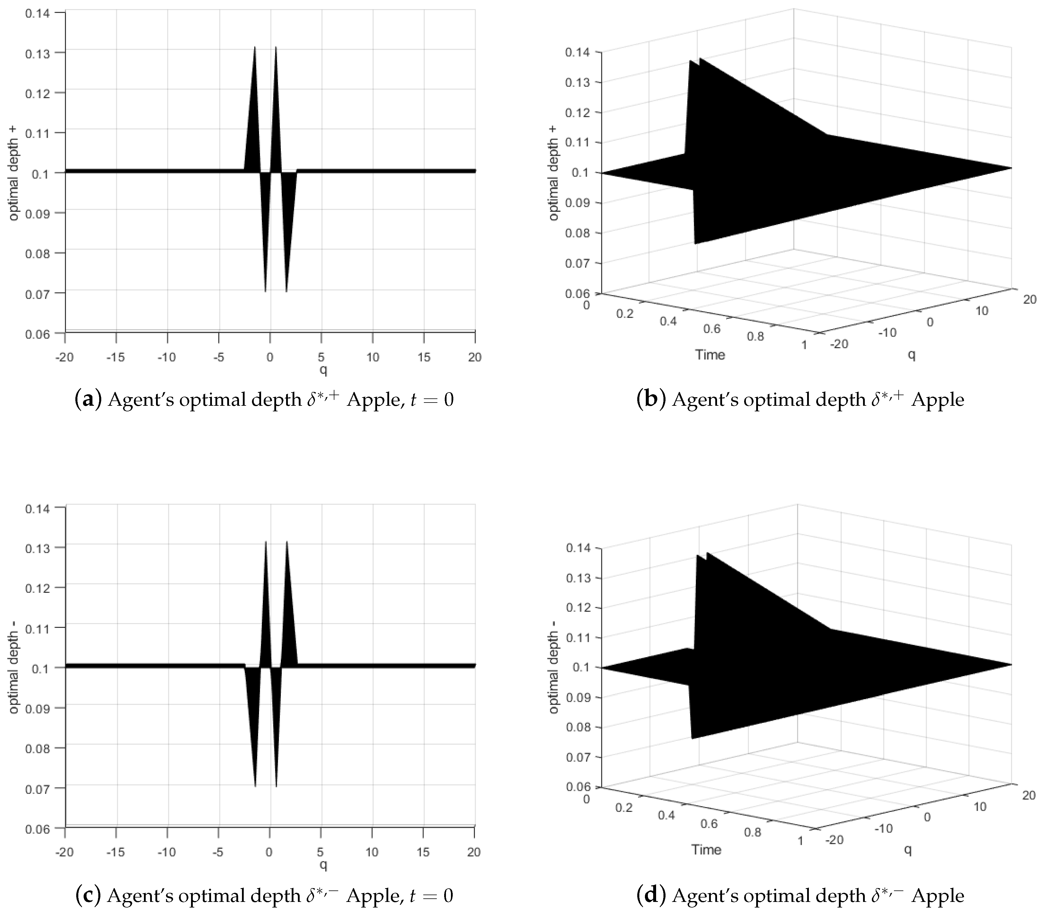
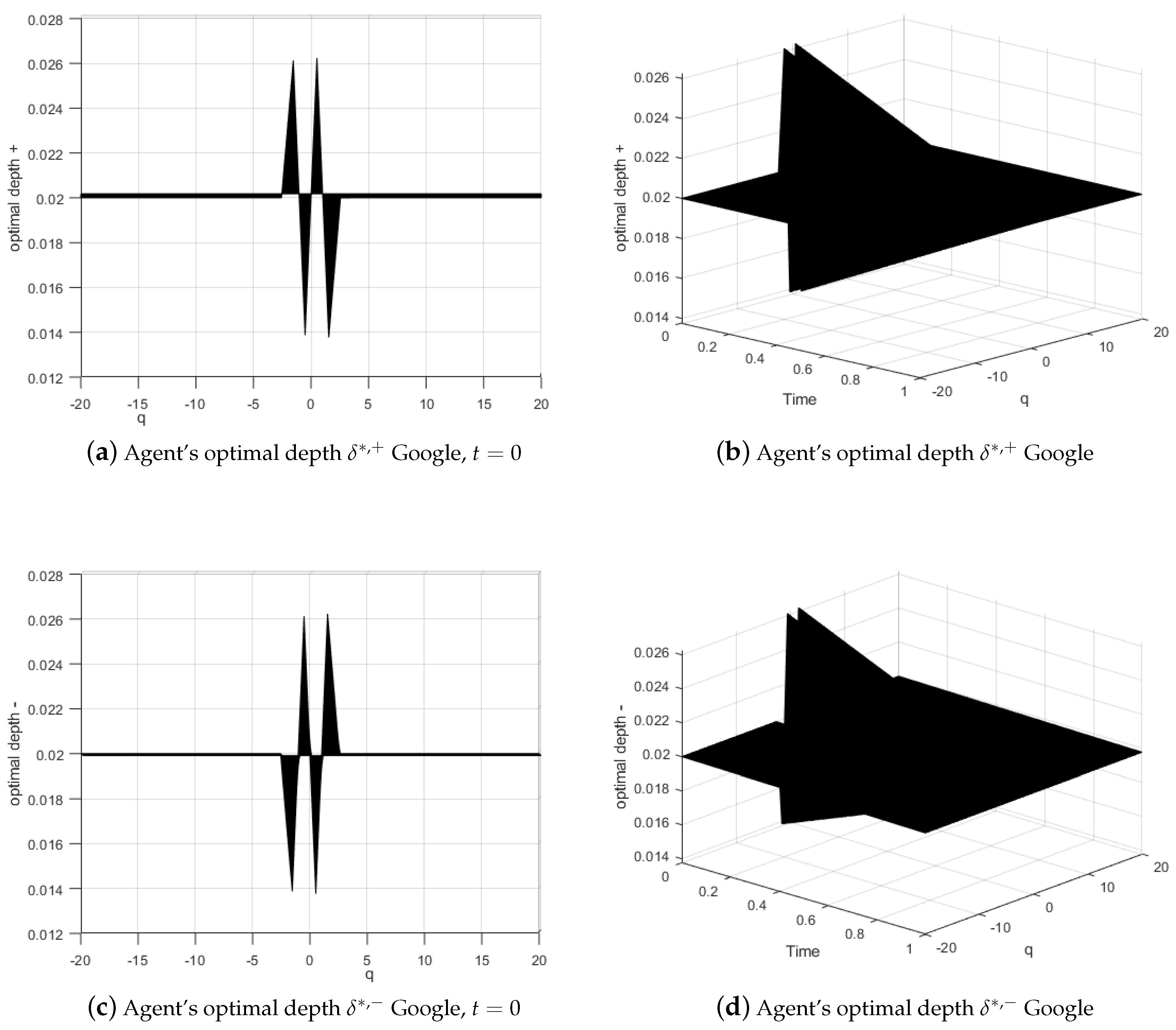
Finally, going back with the construction, we can obtain the optimal depths for the market-making problem, as in Equations (94) and (95).

$$h(t,q)=\frac{1}{\kappa }log\left(exp\left((T-t)·B\right)·Z+Z·D\left(t\right)\right)$$

(93)

$${\delta }^{+,*}(t,q)=\frac{1}{\kappa }-h(t,q-1)+h(t,q),q\ne \underset{¯}{q}$$

(94)

$${\delta }^{-,*}(t,q)=\frac{1}{\kappa }-h(t,q+1)+h(t,q)+2a^{*}\frac{\lambda }{1-\mu }t,q\ne \overline{q}$$

(95)

${\delta }^{+,*}$ and ${\delta }^{-,*}$ give the optimal strategy for every t for different inventory levels. This result is a generalization of the results in Cartea et al. (2015) because it allows the price to be driven by a compound Hawkes process. The optimization contains the compound Hawkes process parameters $\lambda$ and $\mu$. The impact on the price has a direction according to whether it is a buy or sell posting.

In Section 6.5, we present numerical results using the observed price data for Apple, Amazon, and Google on 21 June 2012 (LOBster data) LOBster (2012) and the parameter calibration of parameters $a\ast$ and $\frac{\lambda }{1-\mu }$ from Swishchuk and Huffman (2020) for the GCHP2SDO. We calculated the optimal market-making strategy for an agent’s trading rate, ${\nu }^{*}$, and the optimal depth ${\delta }^{*,\pm }$. In Section 6.5, the results are drawn to show the behavior of the optimal strategy throughout the time available. The parameters used for k, b, $\varphi$, $\alpha$, $\mathfrak{N}$, T, $\kappa$, and ${\lambda }^{\pm }$ are shown in the tables of each stock, according to the model and the asset drawn.

6. Numerical Results with Real Data

In this section, we demonstrate the implementation of the new optimized strategies solved in Section 3, Section 4 and Section 5. We applied our results to real order book data collected from LOBster academic-data LOBster (2012). We considered level 1 and executed operations (meaning limit orders at the best ask and bid price, where the event types were 4 and 5) in this database for Apple, Amazon, and Google on 21 June 2012. The parameter calibration of the general compound Hawkes process for the parameters $a\ast$ and $\frac{\lambda }{1-\mu }$ was taken from Swishchuk and Huffman (2020) for the GCHP2SDO. We calculated the optimal liquidation, acquisition, and market-making strategies for the agent’s trading rate, ${\nu }^{*}$, and the optimal depth ${\delta }^{*,\pm }$.

In the figures below, the results are drawn to show the behavior of the optimal strategy throughout the time available and to explain how to use this model in practice. The parameters used for k, b, $\varphi$, $\alpha$, $\mathfrak{N}$, T, $\kappa$, and ${\lambda }^{\pm }$ are shown in the tables of each stock, according to the model and the asset drawn. The fixed parameters were changed in order to show the adaptability of the results.

6.1. LOBster Data

LOBster is an online limit order book data tool designed to provide easy-to-use, high-quality limit order book data. LOBster data generate a “message” and an “orderbook” file for each active trading day of a selected ticker. The “orderbook” file contains the evolution of the LOB up to the requested number of levels. The “message” file contains indicators for the type of event causing an update of the LOB in the requested price range. All events are timestamped to seconds after midnight, with a decimal precision of at least milliseconds and up to nanoseconds, depending on the requested period. The liquidity of these data is presented in

Table 1. Stock liquidity of AAPL (Apple), AMZN (Amazon), and GOOG (Google) for 21 June 2012 (Swishchuk and Huffman 2020).

Ticker	Avg # of Orders per Second	Price Changes in 1 Day
AAPL	51	64,350
AMZN	25	27,557
GOOG	21	24,084

and Figure 1.

6.2. Main Findings

• The trading rate for the optimal liquidation was sensitive to the parameters of the GCHP driving the prices through $\zeta$ in Equation (26). In this case, as the calibrated $a^{*}$ values were too small, the effect was diminished.
• The parameter $\varphi$, the running inventory penalty, in the optimal liquidation model was changed for the three stocks. We noted, in regard to $\varphi$, that as this parameter increased, the time taken for the agent to deplete their inventory decreased (see Figure 2, Figure 3 and Figure 4).
• As mentioned in Section 4, the trading rate for the optimal acquisition was a constant proportion over time, leading us to obtain $\mathfrak{N}$ in the time T.
• The trading rate for the optimal acquisition was sensitive to the parameters of the GCHP driving the prices through the equation of $ϵ$ in Equation (51). The trading rate was higher according to the structure of the solution and the values of the calibrated parameters; this is in contrast with the results presented in Cartea et al. (2015) using a price model of the general stationary Gauss–Markov process.
• The parameter $\alpha$, the terminal liquidation penalty, in the optimal acquisition model was changed for the three stocks. We were able to visualize the effects of $\alpha$. As this parameter increased, the trading acquisition rate increased and we observed that if $\alpha$ was very small, the agent could not complete the inventory $\mathfrak{N}$ (see Figure 5, Figure 6 and Figure 7).
• The depth in limit orders for the optimal market-making model was sensitive to the parameters of the GCHP, driving the prices from many sides, the matrix $D\left(t\right)$ in the solution, and specifically from the depth to the buy side of LOs, ${\delta }^{*,-}$. In this case, the greater the expected value of the GCHP, the deeper the LO should be placed.
• The parameter $\kappa$, the main factor affecting the probability of filling limit orders in the optimal market-making model, was changed for the three stocks. We were able to visualize the effects of $\kappa$. As this parameter increased, the depth for the LO price on the buy or sell side decreased (see Figure 8, Figure 9 and Figure 10).
• It was interesting to visualize how, in the optimal market-making model, different levels of inventory q led to a curve with four inflection points for the optimal depth in prices (see subfigrues (a) and (c) of Figure 8, Figure 9 and Figure 10).
• As the time in the optimal market-making model grew to T, the optimal depth decreased in a linear way to a positive optimal depth in the long run (see subfigrues (b) and (d) Figure 8, Figure 9 and Figure 10).

6.3. Numerical Results for Optimal Liquidation Problem

We calculated the optimal liquidation strategy for an agent’s trading rate, ${\nu }^{*}$ for Apple stock on 21 June 2012, see

Table 2. Liquidation parameters for Apple stock.

Parameter	Value Used	Parameter	Value Used
T	1	k	$0.001$
b	$0.001$	$\mathfrak{N}$	1
$\alpha$	100	$\frac{\lambda }{1-\mu }$ *	$2.4840$
a *	−$1.1463\times {10}^{-5}$	$\varphi$	$0.001$

* This parameter was calibrated in Swishchuk and Huffman (2020).

and Figure 2.

We calculated the optimal liquidation strategy for an agent’s trading rate, ${\nu }^{*}$ for Amazon stock on 21 June 2012, see

Table 3. Liquidation parameters for Amazon stock.

Parameter	Value Used	Parameter	Value Used
T	1	k	$0.001$
b	$0.001$	$\mathfrak{N}$	1
$\alpha$	100	$\frac{\lambda }{1-\mu }$ *	$1.1110$
a *	−$2.7373\times {10}^{-5}$	$\varphi$	$0.01$

* This parameter was calibrated in Swishchuk and Huffman (2020).

and Figure 3.

We calculated the optimal liquidation strategy for an agent’s trading rate, ${\nu }^{*}$ for Google stock on 21 June 2012, see

Table 4. Liquidation parameters for Google stock.

Parameter	Value Used	Parameter	Value Used
T	1	k	$0.001$
b	$0.001$	$\mathfrak{N}$	1
$\alpha$	100	$\frac{\lambda }{1-\mu }$ *	$0.8857$
a *	−$1.4301\times {10}^{-4}$	$\varphi$	$0.1$

* This parameter was calibrated in Swishchuk and Huffman (2020).

and Figure 4.

6.4. Numerical Results for Optimal Acquisition Problem

We calculated the optimal acquisition strategy for an agent’s trading rate, ${\nu }^{*}$ for Apple stock on 21 June 2012, see

Table 5. Acquisition parameters for Apple stock.

Parameter	Value Used	Parameter	Value Used
T	1	k	$0.001$
b	1000	$\mathfrak{N}$	1
$\alpha$	$0.01$	$\frac{\lambda }{1-\mu }$ *	$2.4840$
a *	−$1.1463\times {10}^{-5}$

* This parameter was calibrated in Swishchuk and Huffman (2020).

and Figure 5.

We calculated the optimal acquisition strategy for an agent’s trading rate, ${\nu }^{*}$ for Amazon stock on 21 June 2012, see

Table 6. Acquisition parameters for Amazon stock.

Parameter	Value Used	Parameter	Value Used
T	1	k	$0.001$
b	1000	$\mathfrak{N}$	1
$\alpha$	$0.1$	$\frac{\lambda }{1-\mu }$ *	$1.1110$
$a^{*}$	−$2.7373\times {10}^{-5}$

* This parameter was calibrated in Swishchuk and Huffman (2020).

and Figure 6.

We calculated the optimal acquisition strategy for an agent’s trading rate, ${\nu }^{*}$ for Google stock on 21 June 2012, see

Table 7. Acquisition parameters for Google stock.

Parameter	Value Used	Parameter	Value Used
T	1	k	$0.001$
b	1000	$\mathfrak{N}$	1
$\alpha$	$0.01$	$\frac{\lambda }{1-\mu }$ *	$0.8857$
a *	−$1.4301\times {10}^{-4}$

* This parameter was calibrated in Swishchuk and Huffman (2020).

and Figure 7.

6.5. Numerical Results for Optimal Market-Making Problem

We calculated the optimal market making strategy for an agent’s optimal depth, ${\delta }^{*,\pm }$ for Apple stock on 21 June 2012, see

Table 8. Market-making parameters for Apple stock.

Parameter	Value Used	Parameter	Value Used
T	1	$\kappa$	10
${\lambda }^{\pm }$	$0.833$	$\mathfrak{N}$	1
$\varphi$	$0.1$	$\frac{\lambda }{1-\mu }$ *	$2.4840$
a *	−$1.1463\times {10}^{-5}$	$\alpha$	1
$\underset{¯}{q}$	$-20$	$\overline{q}$	20

* This parameter was calibrated in Swishchuk and Huffman (2020).

and Figure 8.

We calculated the optimal market making strategy for an agent’s optimal depth, ${\delta }^{*,\pm }$ for Amazon stock on 21 June 2012, see

Table 9. Market-making parameters for Amazon stock.

Parameter	Value Used	Parameter	Value Used
T	1	$\kappa$	20
${\lambda }^{\pm }$	$0.833$	$\mathfrak{N}$	1
$\varphi$	$0.1$	$\frac{\lambda }{1-\mu }$ *	$1.1110$
a *	−$2.7373\times {10}^{-5}$	$\alpha$	1
$\underset{¯}{q}$	$-20$	$\overline{q}$	20

* This parameter was calibrated in Swishchuk and Huffman (2020).

and Figure 9.

We calculated the optimal market making strategy for an agent’s optimal depth, ${\delta }^{*,\pm }$ for Google stock on 21 June 2012, see

Table 10. Market-making parameters for Google stock.

Parameter	Value Used	Parameter	Value Used
T	1	$\kappa$	50
${\lambda }^{\pm }$	$0.833$	$\mathfrak{N}$	1
$\varphi$	$0.1$	$\frac{\lambda }{1-\mu }$ *	$0.8857$
a *	−$1.4301\times {10}^{-4}$	$\alpha$	1
$\underset{¯}{q}$	$-20$	$\overline{q}$	20

* This parameter was calibrated in Swishchuk and Huffman (2020).

and Figure 10.

7. Conclusions

In this paper, we solved the optimal liquidation, acquisition, and market-making problems in the high-frequency trading market. We designed the problems to work along with a special price modeled using a general compound Hawkes process and its diffusion results. The results showed themselves to be sensitive to the parameters of the GCHP driving the prices, which are important characteristics that reflect the behavior of real-world price processes such as the dependence on the previous process and jumping attributes. In these models, the agent maximized their value function by solving the Hamilton–Jacobi–Bellman (HJB) equation to design a strategy for asset trading. The optimal solutions were expressed based on the parameters for the arrival rates and the midprice process, modeled as a GCHP. The visualization of the LOBster data and how the optimal solutions worked granted a better understanding of the models. Furthermore, it enabled us to explain in a clear way the importance of certain critical parameters working in the models and how they affected the optimized results. We were also able to realize how the calibrated midprice process could be used to adjust the trader’s response by looking at the arrival rates and depth of prices in the LOB.

8. Discussion and Future Work

After reviewing our results and those of previous works, it is important to remark that the GCHP is a more general model, meaning that it can be structured to have Markovian properties and imitate the behavior of contrasting price models. Thus, we can say that it has an advantage over those models in that it can adjust in an extended way to the behavior of the real-world prices in HFT, resulting in more flexible optimized models. These new optimized processes, calculated in this paper, can be compared with the general stationary Gauss–Markov process used in Cartea et al. (2015) and also with the Markov renewal process adopted by Fodra and Pham (2015), as well as the Cox–Ingersoll–Ross model operated by Fruth et al. (2019). These optimization problems are based on different price models. There are arguments for and against the use of these price models, which have been detailed in the introduction, and now with the solutions provided by the GCHP approach, we can see that the optimized values contain relevant characteristics from the real-world prices in HFT. These models have the limitation of working with approximations for GCHP, such as LLN and FCLT. This paper is a first step towards solutions obtained with the infinitesimal generator of the GCHP.

There are many directions of research that could be followed after obtaining these results. These models worked with the use of diffusion approximations for GCHP. In future research, we suggest working with diffusion approximations for semi-Markovian models such as those described in Swishchuk et al. (2017). These processes allow new book events to depend on the previous event, preserving the advantageous properties of Markov chains. This could illustrate other characteristics of real-world prices. Furthermore, working with the actual GCHP and its infinitesimal generator to solve optimization problems represents a harder challenge, given that the infinitesimal generator has to be defined according to the counting process, the distribution of the interarrival times, and the transition probabilities. In future works, we will aggregate these important steps to contribute to the literature on mathematical finance in HFT markets.