Interpolation of Quantile Regression to Estimate Driver’s Risk of Traffic Accident Based on Excess Speed

Abstract

Quantile regression provides a way to estimate a driver’s risk of a traffic accident by means of predicting the percentile of observed distance driven above the legal speed limits over a one year time interval, conditional on some given characteristics such as total distance driven, age, gender, percent of urban zone driving and night time driving. This study proposes an approximation of quantile regression coefficients by interpolating only a few quantile levels, which can be chosen carefully from the unconditional empirical distribution function of the response. Choosing the levels before interpolation improves accuracy. This approximation method is convenient for real-time implementation of risky driving identification and provides a fast approximate calculation of a risk score. We illustrate our results with data on 9614 drivers observed over one year.

1. Introduction

Our motivation for this paper is to adjust the risk level of drivers using car insurance telematics data. We focus on one of the most widely accepted indicators of dangerous driving, which is total yearly distance driven above posted speed limits (Aarts and Van Schagen 2006; Elliott et al. 2003). If all drivers had identical characteristics, direct one-to-one comparisons could be sufficient to identify dangerous individuals, but since drivers are not completely identical and they operate in a variety of circumstances, additional covariate information needs to be considered when assessing their risk. For example, among other things, someone driving 10,000 km per year has a higher risk of exceeding speed limits, and thus of having an accident during one year, than someone driving only occasionally. Our premise is that we should take into consideration explanatory variables when addressing risk scores.

Quantile regression (Koenker and Bassett 1978) is a suitable method for finding conditional risk scores and therefore it is a good instrument for our purposes (Pérez-Marín et al. 2019; Guillen et al. 2020). However, estimating quantile regressions is computationally demanding in large databases when many covariates are considered (Chen and Zhou 2020). A driver’s risk score is defined as the quantile level at which the estimated conditional quantile is equal to the observed response. In order to fit a risk score to each driver, many quantile regressions need to be estimated. In real-time applications with many incoming new data, updating, re-estimation, and performing repetition of quantile regression estimation is way too slow. Some algorithms that suggest to obtain parameter estimates with one-step approximations may not be reliable for extreme quantile levels (Chernozhukov et al. 2020).

Here we develop a simple approximation method based on interpolation that is able to provide a fast approximation to quantile estimation of neighbouring levels and ultimately to furnish a fast estimate of the risk score for each individual in our pool, given their current observed exogenous characteristics. In our case study, this method allows the identification of drivers with a high risk of exceeding speed limits conditional on their covariate information.

This study proposes an approximation of quantile regression coefficients by interpolating only a few quantile levels, which can be chosen carefully from the unconditional empirical distribution function of the response. Choosing the levels before interpolation improves accuracy. This approximation method is convenient for real-time implementation of risky driving identification and provides a fast approximate calculation of a risk score.

Since we know that driving speed is associated with accident risk, our method is a dynamic instrument that is suitable for establishing alerts and warnings to take precautions. It can also be applied to other continuous responses, like average speed or night-time driving, and in other contexts. Risk scores are needed in many fields, ranging from industrial production to household protection, where they play a major role for future innovations; however, the area of traffic accident analysis provides an excellent landscape for our illustration because big databases are widely available.

During the last few decades, telematics data have become increasingly popular because motor insurance companies have been interested in personalizing prices for their customers. Data are collected through on-board devices or via mobile phones. Different methods are used to adjust insurance prices. Pay-as-you-drive (PAYD) is a method that has already been implemented in the market in many countries around the world. PAYD means that insurance cost is based on distance driven. Pay-how-you-drive (PHYD) also considers available information on driving style. In PHYD, the price is based on relevant information about driving patterns and may increase when dangerous indicators arise (Guillen et al. 2021; Sun et al. 2021). Another insurance pricing method that is still under development is known as manage-how-you-drive (MHYD). In this case, there should be some kind of feedback to the customer almost in real time to provide information on driving issues that can be used to improve safety and, ultimately, to reduce the cost of insurance. Insurance companies claim that customers are not yet prepared to accept MHYD systems, but the truth is that implementation of MHYD systems would require fast algorithms that are able to forward knowledge from data in a dynamic way that is valuable both for the customer and for the company.

In our case study, we model the number of kilometres driven above the posted speed limit over one year as a function of driving characteristics and we also include the driver’s personal information, such as gender and age. We consider that our response variable of interest is strongly linked with the risk of having a traffic accident. Using quantile regression, each driver was scored as follows: firstly, for each quantile level (percentile) from 1% to 99%, we compare the fitted conditional quantile with the driver’s observed response value. Then we calculate the driver’s risk score as the percentile level that minimizes the difference between the estimated conditional quantile and observed value. A score close to 100% indicates that that the driver has a high risk. This is so because the number of kilometres driven above the legal speed limit is similar to a high conditional quantile. Therefore, the driver is much more risky than other drivers with similar characteristics. Conversely, a score that is close to 0% indicates that the driver’s observed value corresponds to a low conditional quantile. That means that this driver is safer than other drivers with similar covariate information.

The main computational burden when fitting risk scores arises in the first step, because many quantile regressions need to be fitted. This step is necessary to adjust quantiles at all levels and then to find the level that provides the minimum difference between the estimated conditional quantile and the observed response. If implemented in databases with a large number of cases and to models with a lot of variables, fitting percentiles through quantiles regressions requires computational time. To solve this, we propose fitting only a reduced number of quantile regressions and to approximate all other quantile regression parameter estimates by interpolation. We determine the minimum number of regressions to be fitted in order to obtain accurate predictions of the risk scores by minimizing mean squared error. Obtaining fast approximations is crucial to ensuring the applicability in dynamic schemes, as it will lead to improvements in terms of computational time. In this paper, we study the performance of our approximation depending on the number of adjusted quantile regressions in a real case study. We conclude that for extreme values, the number of adjusted regressions has a high impact on the accuracy of the predictions. In general, as the number of fitted quantile regressions increases, the risk score fit is more accurate, but more time-demanding.

The paper proceeds as follows. First, we present a literature review of papers that study risks of traffic accidents from different points of view. We then present quantile regression and the interpolation method used to estimate quantile parameters at intermediate levels. After the methodology, we present the data used in our case study section and we discuss the results when fitting quantile regression models and determining the minimum number of regressions required to produce risk scores. The last section concludes the paper.

2. Literature Review

Smith (2016) studied the relationship between having an accident and driving patterns. He also considered the risk taken while driving and, in particular, when the driver is fatigued. He conducted a qualitative study in a survey in the UK. A similar study was performed by Singh (2017), who used information about multiple traffic accidents in India to understand which scenarios correlate with a higher risk of having a road accident. He considered the weather and location of the crash and discussed solutions to lower the number of accidents. Guillen et al. (2020) studied the use of reference charts to estimate the percentiles of distance driven at high speed. Reference charts are a standard approach to study the weight and height of children, and the same principles are used in telematics data. The authors fitted quantile regression models at different quantiles using covariates that reflect driving patterns. They found that total distance driven, gender and percent of urban driving are important factors explaining distance driven above speed limits. They also found that the relationship between total distance driven and total distance driven above the legal speed limit is relevant to produce a reference chart and a better fit of the percentiles. Sun et al. (2020, 2021) adjusted ordinary least squares and binary logistic regressions to calculate a driving risk score for different drivers using internet of vehicles (IoV) data. Usage-based insurance is a new methodology based on IoV that is being used to customize insurance prices. However, their method requires a good identification of risky drivers. They found that revolutions per minute, average speed, braking events and accelerations are important variables for identifying risky drivers, while other GPS related variables do not provide a lot of information. Pérez-Marín et al. (2019) also studied the risk of speedy driving adjusting quantile regressions at different quantile levels. They used information related to driving patterns as in (Guillen et al. 2020), but they focused on the differences in the effects of explanatory variables at different quantile levels. They concluded that total distance driven, night driving, urban driving, gender and age are important factors in the risk of speedy driving and proposed quantile regression as a methodology to be considered when calculating motor insurance rates. Guillen et al. (2019) studied a sample in which there was a high number of drivers with zero accident claims, so they needed to adjust a zero-inflated Poisson model when modelling the number of accidents. They proposed a methodology to improve the design of insurance. They analysed all reported claims and only those where the driver was at fault. When all claims were analysed, gender, driving experience, vehicle age, power of the vehicle, distance driven at high speed and urban driving significantly affected the risk of accident. But when only accidents at fault were analysed, neither gender nor engine power had a significant effect. The authors highlighted the importance of total distance driven over one year when analyzing the risk of accidents and discussed the role of distance in PAYD insurance schemes.

Many recent contributions advocate using techniques from machine learning, deep learning and pattern recognition to the analysis of telematics data (Weidner et al. 2016; Gao and Wüthrich 2018, 2019; Gao et al. 2018). These papers aim at classifying drivers by means of raw telematics information. Boucher and Turcotte (2020) study the relationship between claim frequency and distance driven through different models by observing smooth functions. They show that distance driven and expected claim frequency seem to be approximately linearly related and argue that this is the basis to construct pay-as-you-drive (PAYD) insurance schemes. More recently, Henckaerts (2021) emphasizes the interest of dynamic pricing with telematics collected driving behavior data.

A relatively high number of papers relate traffic accident risk not to driving patterns but to the driver’s specific health conditions, which may influence driving style and driving issues. Gohardehi et al. (2018) reviewed papers that studied toxoplasmosis as a potential influence on the risk of having a traffic accident. In a meta-analysis, they use conclusions from studies carried out in different countries to evaluate whether this disease could be a significant risk factor. Huppert et al. (2019) studied the risk of road accident in drivers that had been diagnosed in the previous five years with a disease that can cause vertigo. Drivers were not diagnosed when they took out insurance. Matsuoka et al. (2019) studied whether there is a positive correlation between the number of traffic accidents and the number of epileptic drivers that have sleep-related problems. They considered driver characteristics and the type of epilepsy from which the drivers suffered.

Closer to the aim of this paper, other studies have examined which factors affect the risk of crash by adjusting mathematical models. Mao et al. (2019) used a multinomial logistic regression to identify which factors affect the risk of having a traffic accident in China. They considered four different types of crash depending on the collision characteristics and separated the studied factors into six categories. Rovšek et al. (2017) identified accident risk factors via a Classification and Regression Tree (CART) using data collected from Slovenia that provided information on the conditions at the time the accident happened. Lu et al. (2016) studied agents that affect the severity of traffic accidents with an ordered logit model. Their data contained information about different traffic accidents that occurred in different Shanghai tunnels and included characteristics of the driver, time, weather conditions and site features, but again data were about information on the circumstances of the accident, not driving habits. Eling and Kraft (2020) summarize 52 contributions covering a variety of telematics empirical analyses. The choice of variables seems to be centered on two sources: telematics driving behavior data and policy information including insured characteristics and claiming history. Models usually rely on variables related to vehicle use like distance driven and covariates such as age, gender, driving zone and policy information. A more recent example of a similar choice of variables is (Henckaerts et al. 2021).

With the exception of (Guillen et al. 2020) none of the previous authors used a quantile regression approach to score the driver’s accident risk. As such, the papers included in this review did not focus on the problems posed by iterated, intensive data analysis, like the one we address here.

3. Proposed Methodology

For a continuous random variable Y, quantile $\tau$ ($\tau \in (0,1))$ is defined as:

$$Q_{\tau }\left(Y\right)=inf\{y\in {\mathbb{R}}^{+}:F_Y\left(y\right)>\tau \},$$

(1)

where $F_Y\left(y\right)$ corresponds to the cumulative distribution function of Y and $\tau$ is known as the quantile level. In other words, quantile $\tau$ is the value that is only exceeded by $(1-\tau )$ proportion of observations of Y.

Koenker and Bassett (1978) proposed an extension of linear regression called quantile regression. Quantile regression adjusts the effects of explanatory variables for the $\tau$-th quantile of a response variable. Consider a data set with n observations, where $Y_i$ represents the response variable for the i-th individual observation ($i=1,\dots ,n$) and $X_{ji}$ represents the value of explanatory variable j ($k=1\dots k$) for the i-th individual. A quantile regression model at level $\tau$ is specified as follows:

$$Y_i={\beta }_0^{\tau }+{\beta }_1^{\tau }{X}_{1i}+{\beta }_2^{\tau }{X}_{2i}+\cdots +{\beta }_k^{\tau }{X}_{ki}+{ϵ}_i^{\tau },$$

(2)

where $Q_{\tau }\left({ϵ}_i^{\tau }\right)=0$ and ${\beta }^{\tau }$ is the vector of unknown parameters, and ${\beta }_0^{\tau }+{\beta }_1^{\tau }{X}_{1i}+{\beta }_2^{\tau }{X}_{2i}+\cdots +{\beta }_k^{\tau }{X}_{ki}$ is the linear predictor, which is denoted by $X_i^{\prime }{\beta }^{\tau }$.

Quantile regression models are particularly useful when the response variable is not symmetrical. For example, at $\tau =0.5$ the median of the response, which is robust to outliers, is modelled. This is different to modelling the mean, which is the traditional approach in classical linear regression. Quantile regression can also be specified as the conditional $\tau$-th quantile of $Y_i$ equal to the linear combination of the covariates with the equation:

$$Q_{\tau }\left(Y_i\right|X_i^{\prime }{\beta }^{\tau })={\beta }_0^{\tau }+{\beta }_1^{\tau }{X}_{1i}+{\beta }_2^{\tau }{X}_{2i}+\cdots +{\beta }_k^{\tau }{X}_{ki}.$$

(3)

Koenker and Bassett (1982) and Koenker and Machado (1999) presented the optimization problem to fit a quantile regression model:

$$\widehat{{\beta }^{\tau }}=\underset{{\beta }^{\tau }}{argmin}\sum _{i=1}^n{\rho }_q^{\tau }(Y_i-X_i^{\prime }{\beta }^{\tau }),$$

(4)

where ${\rho }_q^{\tau }$ represents a score function of the quantile that equals $\tau (Y_i-X_i^{\prime }{\beta }^{\tau })$ when $(Y_i-X_i^{\prime }{\beta }^{\tau })\ge 0$ and $(\tau -1)(Y_i-X_i^{\prime }{\beta }^{\tau })$, otherwise.

3.1. Interpolating the Parameter Estimates

Suppose that after fitting quantile regressions (3) for levels $\tau =0.01,\dots ,0.99$, we want to identify each observation i with the corresponding $\tau$ level that provides an estimated quantile close to the observed response value. To adjust the quantile value we will solve the following optimization problem:

$${\widehat{\tau }}_i=\underset{\tau }{argmin}{(Y_i-X_i^{\prime }{\beta }^{\tau })}^2,$$

(5)

where ${\beta }^{\tau }$ will be replaced by their corresponding parameter estimates $\widehat{{\beta }^{\tau }}$. The objective function represents the difference between the observed value of the response variable and the fitted $\tau$-quantile value of the response given characteristics of individual i. The ideal scenario to solve this problem is to have a large set of adjusted quantile regressions, ideally as many $\tau$ as possible, in order to find the optimal $\tau$. Note that the optimization problem may turn into numerical instabilities because for any ${\tau }_a<{\tau }_b$ it is not necessarily true that $X_i\widehat{{\beta }^{{\tau }_a}}<X_i\widehat{{\beta }^{{\tau }_b}}$, so there may be local minima. In that case we would choose the smallest ${\widehat{\tau }}_i$ providing the minimum loss.

Having a large number of $\widehat{{\beta }^{\tau }}$ is non-viable when databases have a massive number of observations and when we are trying to fit a quantile regression model with a large number of variables. In this paper we want to show that only a few quantile regressions are required to obtain an accurate estimation of ${\widehat{\tau }}_i$, i = $1,\dots ,n$ without modelling for hundreds of quantile levels, and thus saving computing time.

We first fit 99 regressions, one for each $\tau$ corresponding to percentiles 1 to 99, and then we select $m<99$ regressions that have equidistant $\tau$ levels. When approximating ${\widehat{\beta }}^{{\tau }_0+c}$, we select two consecutive values of $\widehat{{\beta }^{\tau }}$ considering ${\tau }_0$ which represents the lower selected quantile level, ${\tau }_1$ which represents the upper selected quantile level and $c\in (0,({\tau }_1-{\tau }_0))$. For example, for $m=6$, $\tau \in \{0.01,0.2,0.4,0.6,0.8,0.99\}$. To interpolate the values of $\widehat{{\beta }^{\tau }}$ for $\tau \notin \{0.01,0.2,0.4,0.6,0.8,0.99\}$, we use the formula:

$${\widehat{\beta }}^{{\tau }_0+c}=\frac{{\beta }^{{\tau }_0}+c({\beta }^{{\tau }_1}-{\beta }^{{\tau }_0})}{{\tau }_1-{\tau }_0}.$$

(6)

To compare the performance of the approximating method, we calculate the Mean Square Error (MSE) as follows:

$$MSE=\frac{{\sum }_{i=1}^n{({\widehat{\tau }}_i^{99}-{\widehat{\tau }}_i^m)}^2}{n},$$

(7)

where n is the number of observations in the data set, ${\widehat{\tau }}_i^{99}$ is the fitted score for the i-th observation when adjusting 99 quantile regressions and ${\widehat{\tau }}_i^m$ represents the adjusted $\tau$ for the i-th observation adjusting only m regressions and interpolating the coefficients for the other percentiles.

3.2. Adapted Choice of Quantile Levels before the Approximation

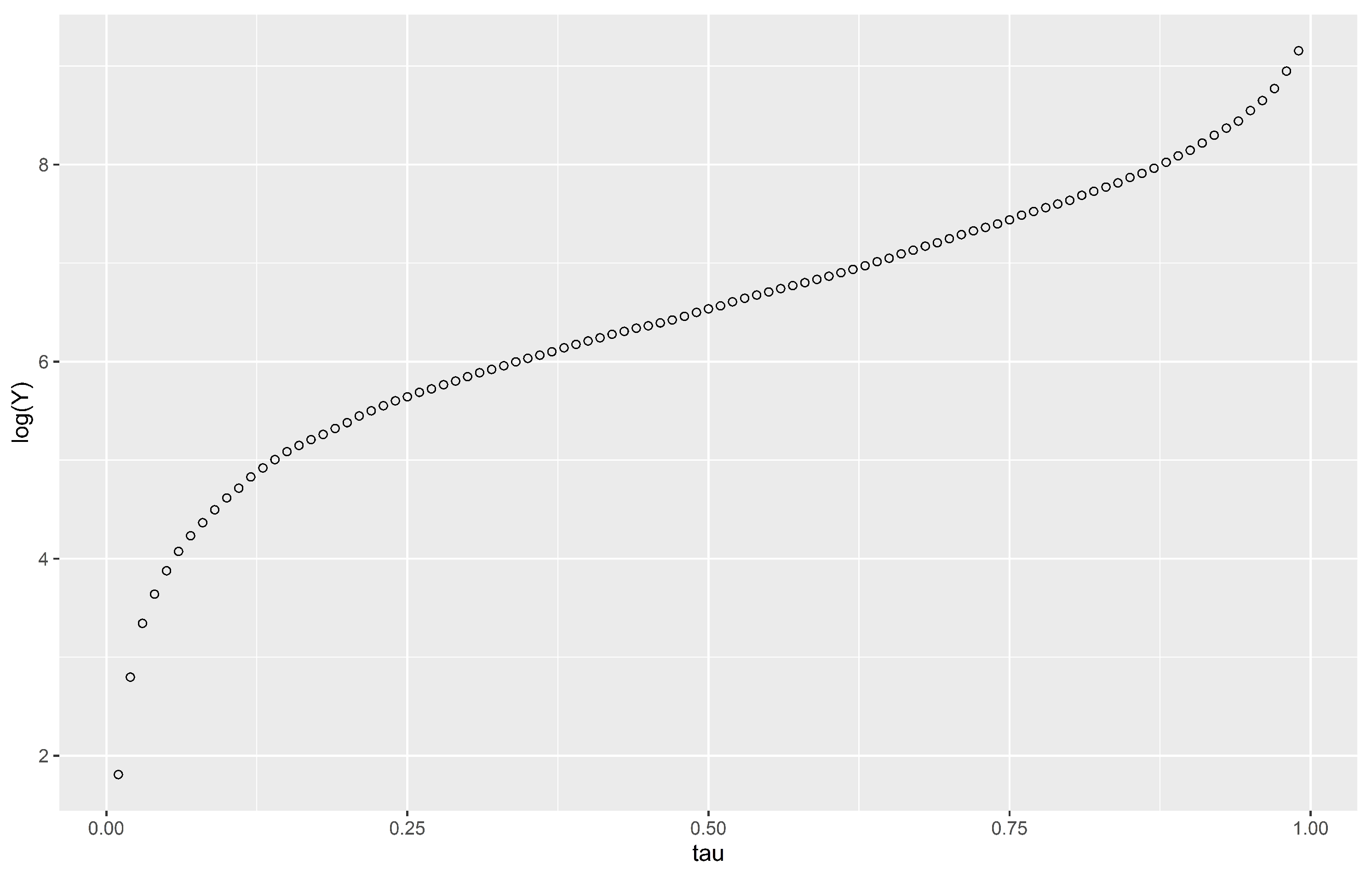
Using the methodology proposed to interpolate quantile regression coefficients for those levels that were not estimated, in the previous subsection we propose choosing m regressions with $\tau$ values that are equidistant, allowing us to fit the same number of regressions in those parts of the distribution of the response variable that are flatter than others. This can be visualized in an example quantile function provided in Figure 1. Figure 1 shows that for the lower quantile levels the response (here presented in logarithm) rises rapidly, then the increase is constant and then for higher quantile levels the increase is once again rapid.

Considering that when we work with quantile regression we establish a linear relationship between the quantiles and the effects of covariates, it turns out that determining which zones of the quantile function require more attention is crucial to improve on the accuracy of the approximation. Figure 1 shows that we should adjust more quantile regressions for lower levels where the distribution changes more rapidly than in the middle levels. Therefore, fewer fits are needed for the central part of the distribution because the increase is linear in that part of the domain. Increasing the number of regressions adjusted at some part of the distribution, which is equivalent to deciding adequate $\tau$ levels or changing the distance between the concrete $\tau$ values, may considerably improve the accuracy of the results.

4. Data and Results

Telematics data have become increasingly relevant in recent years. In the field of motor insurance, they are used to provide personalized prices to customers depending on their driving patterns. In this paper we use a database containing information about 9614 drivers aged between 18 and 35 years. The information on each driver includes total distance driven, time of the day, type of road and distance driven above the legal speed limit over one year. It also contains information about the driver’s personal characteristics such as age and gender. All information contained in the database was collected during 2010. The variables in the dataset are defined in

Table 1. Definition of variables in the telematics data set for 2010.

Variable	Description
Speed_km *	Total number of kilometres driven above the legal speed limit
lnKm	Logarithm of the total number of kilometres driven
P_urban	Percentage of kilometres driven in urban areas
P_night	Percentage of kilometres driven at night
Age	Age of the driver
Male	Gender of the driver (1 = male, 0 = female)

* P_speed is the proportion (percentage) of total kilometres driven above the speed limit. P_speed = 100 × Speed_km /exp(lnKm).

.

In

Table 2. Descriptive analysis of the continuous variables in the telematics data set for 2010 ($n=9618$).

	Mean	Median	Min.	Max.	Std. Dev.
Speed_km	1398.21	689.23	0.00	23,500.19	1995.37
lnKm	9.27	9.37	−0.37	10.96	0.75
P_urban	26.29	23.39	0.00	100.00	14.18
P_night	7.02	5.31	0.00	78.56	6.13
Age	24.78	24.63	18.11	35.00	2.82

we present a descriptive statistical analysis. The sample contains 4873 males and 4741 females. As usual in this context, we consider total distance driven on a logarithmic scale. Our response variable is the number of kilometres driven above the speed limit. This variable is positively correlated with accident risk and it is quite asymmetrical. This is the reason why quantile regression is particularly suited to our analysis.

Other studies have used this database. Ayuso et al. (2016) compared driving patterns between males and females and Guillen et al. (2019) proposed a new methodology to determine the insurance price. Boucher et al. (2017) analysed the effects of distance driven and the exposure time on the risk of having a traffic accident using generalized additive models (GAM). Pitarque et al. (2019) used quantile regression to analyse the risk of traffic accident and Pérez-Marín et al. (2019) analysed speedy driving.

Our first objective is to produce quantile regression models for the total number of kilometres driven above the speed limit at percentile levels 1 to 99. This is the first step towards fitting conditional percentiles and identifying which observations correspond to risky drivers given their driving patterns. We work with the logarithm of the response variable following the work of previous authors.

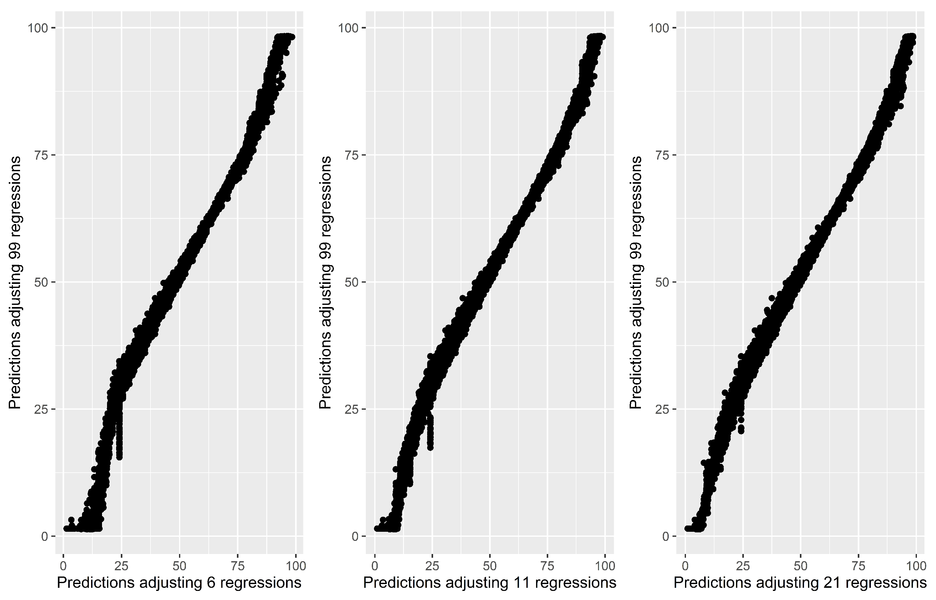
Figure 2 presents each driver in the data set by representing drivers’ risk score (${\widehat{\tau }}_i^{99}$) obtained with 99 regressions versus their fitted score ${\widehat{\tau }}_i^m$, where scores were calculated with the interpolation method (6) with an increasing number (m) of initially adjusted quantile models with equidistant $\tau$ levels.

In Figure 2, the horizontal axis represents the value of $\tau$ risk scores obtained by adjusting m regressions and the vertical axis represents the fitted values obtained by adjusting 99 regressions. We can observe that when adjusting only six quantile regression models (left panel) before the linear interpolation of coefficients, we encounter a significant problem when fitting lower percentile values. In those cases, the approximated value is larger than it should be. There are also some differences in the estimation of the larger quantiles but at a lower magnitude. 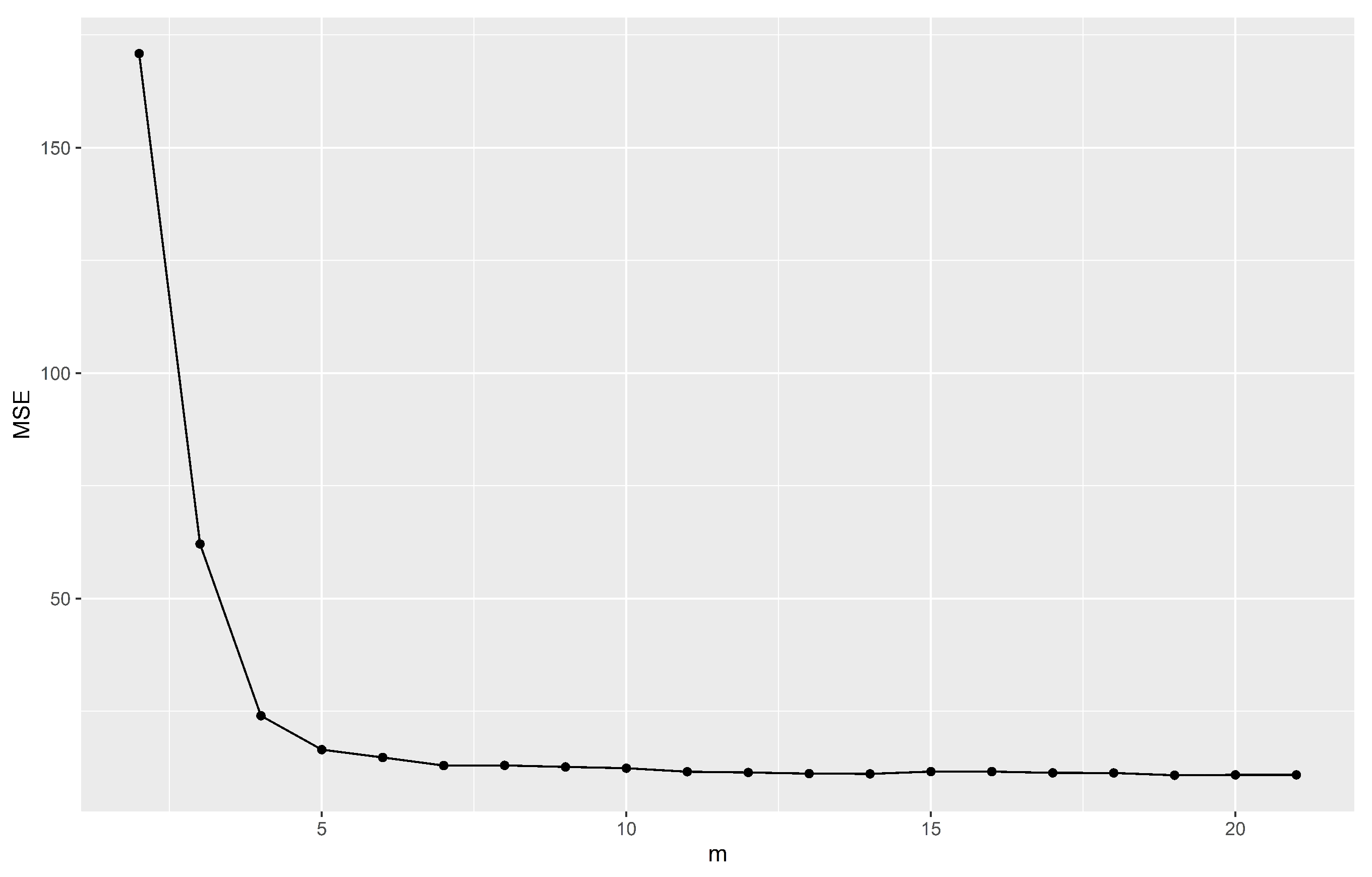Adjusting 11 quantile regressions (middle panel), fitted values for $\tau \in (0.4,0.85)$ are more accurate than before and the problem of fitting extreme values of $\tau$ decreases especially for large values. When adjusting 21 quantile regressions (right panel), we observe that in general all adjusted values are more accurate than the previous two panels, but we still have some discrepancies for lower quantiles. To determine how many regressions are necessary to obtain a good fit we present Figure 3, which shows the behaviour of the $MSE$ defined in (7) as a function of the initial number of fitted quantile regression before the approximation (see also

Table 3. Mean square error ($MSE$), root mean square error ($Root.MSE$) and mean absolute error ($MAE$) for risk score estimates when adjusting m regressions.

m	2	6	9	11
$MSE$	170.890	14.713	12.609	11.545
$Root.MSE$	13.072	3.836	3.551	3.398
$MAE$	10.362	2.949	2.930	2.821
m	13	15	18	21
$MSE$	11.116	11.573	11.264	10.836
$Root.MSE$	3.334	3.402	3.356	3.292
$MAE$	2.771	2.827	2.786	2.735

). Table 3 shows that mean squared error can be used as a criterion to optimize the choice of quantiles levels. Table 3 also displays root mean square error ($Root.MSE$) and mean absolute error ($MAE$).

In Table 3, $MSE$ values decrease when the number of initially adjusted regressions increases and then they stabilize around $m=9$. For $m=11$ there are still some problems for lower risk scores and in general there are no major improvements in the results for $m>11$.

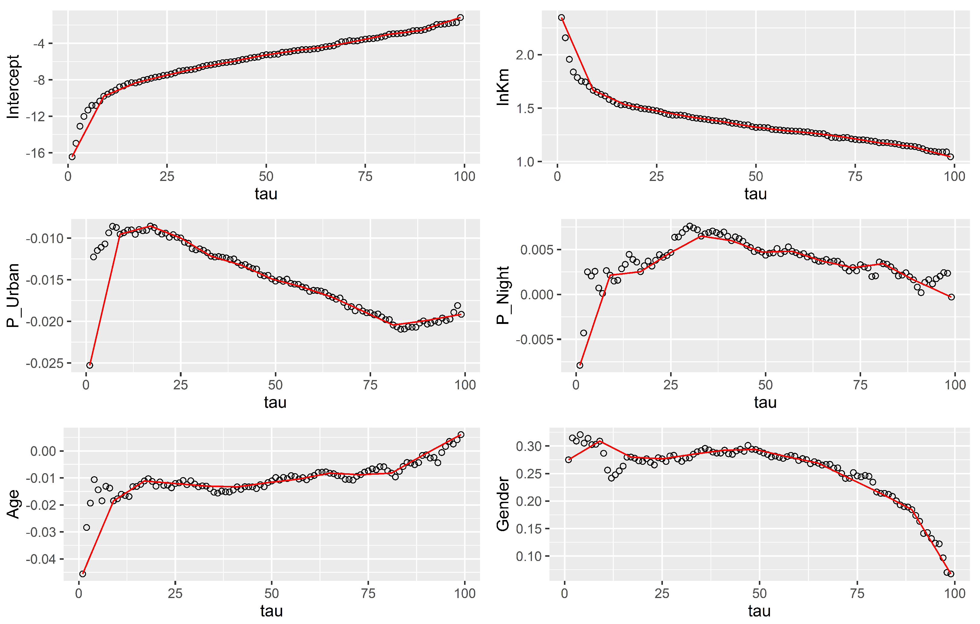
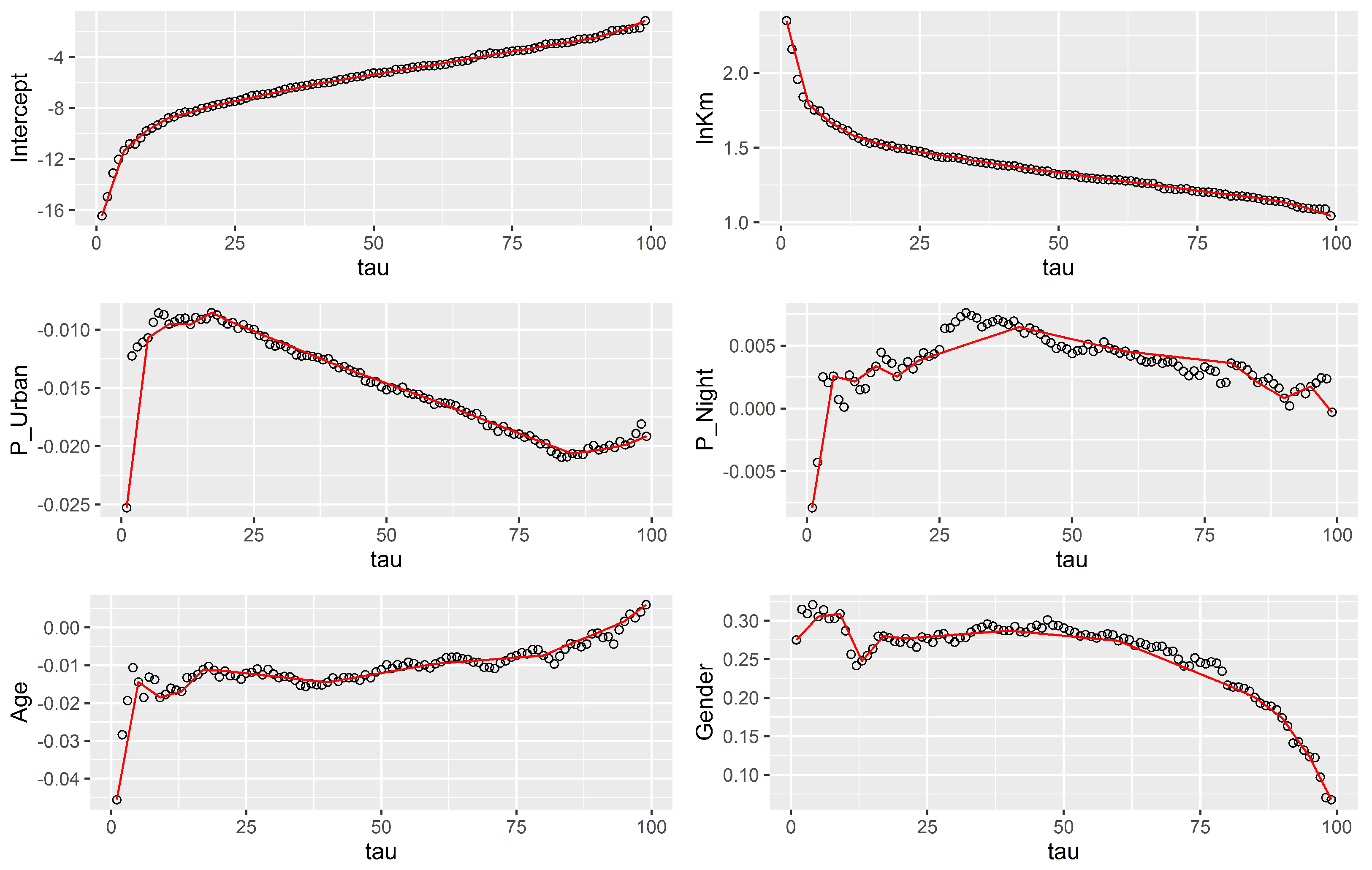
Depending on which m quantile levels were selected for modelling, increases or decreases in $MSE$ are produced. To study the possible causes of fitting problems in low percentiles, in Figure 4 we present the evolution of ${\beta }^{\tau }$ parameters and the extrapolation adjusting $m=13$ regressions; this number had the lowest $MSE$ value for $m<15$.

In Figure 4, we can observe that in general for all covariates, extrapolations do not fit well the parameter estimates for lower quantiles. In all cases except total distance driven, the interpolated value is lower than the estimated coefficient for $m=99$. Since the interpolated value is lower than it should be, a larger value of $\tau$ is required to obtain the minimum value for $Y_i-X_i^{\prime }{\beta }^{\tau }$ and this leads to an overestimation of the risk scores. For upper quantiles, the only covariate that has fitting issues is the percentage of night driving.

Regarding computational time, when adjusting $m=13$ regressions and approximating the rest, it takes 13 s to obtain all fitted values. Adjusting $m=99$ quantile regressions requires 120 s. Thus, we conclude that time-reduction is around order ${10}^{-1}$, which is a major improvement in terms of computational time.

In order to reduce $MSE$, we fitted $m=13$ regressions but selected the quantile levels carefully. We fitted five quantile regressions for $\tau \in [0.01,0.20)$, four quantile regressions for $\tau \in [0.20,0.80)$ and four regressions for $\tau \in [0.80,0.99)$. In this case, unbalancing the distance between $\tau$ levels leads to increasingly accurate extrapolations for ${\beta }^{\tau }$ parameters for the extreme values of $\tau$. Figure 5 presents the new comparison between ${\beta }^{\tau }$ estimations and interpolations; we can see that we solved some problems for the estimation of lower quantile coefficients that appeared in Figure 1 and that we have a nice fit for the rest of the quantile coefficients.

$MSE$ is also affected by the choice of $\tau$ levels. When we approximate ${\beta }^{\tau }$ with our methodology and choose levels carefully as mentioned above, $MSE$ equals $10.057$, which is lower than $11.116$ (see Table 3, for $m=13$ and equally spaced $\tau$ levels). A lower $MSE$ indicates an improvement in the accuracy of our adjusted scores with the approximation method.

5. Discussion

In insurance, it is important to detect which drivers have a major risk of having a traffic accident or bad driving patterns. Adjusting a quantile regression for each quantile level to find which quantile level provides a conditional percentile that equals the observed response has a high computational cost in terms of time. This cost is accentuated when the adjusted model has lots of variables or in databases having a large number of observations. We found that for 9614 observations the computational time was drastically reduced by almost 90% when implementing the approximation algorithm for $m=13$ (from 2 min for 99 regressions to 13 s for 13 regressions and the interpolation, as implemented in R on a standard personal laptop).

We show that our approximation based on fitting only a few quantile regressions instead of all levels provides good results when approximating the regression parameters. Increasing the number of fitted quantile regressions would provide few benefits. Nevertheless, the evolution of ${\beta }^{\tau }$ parameters should be studied in each case to select an appropriate number of initial levels at which the quantile regressions should be estimated. The empirical quantile function of the response variable can also be useful to identify the nature of the unconditional response variable distribution.

We observed that as the number of fitted quantile regressions increased in the first step, ${\beta }^{\tau }$ extrapolated parameters were closer to the true parameters but for lower quantiles there was always a small error that provoked some deviation in our estimated risk score values. Applying the methodology proposed in this paper, we saw that if we select $\tau$ values carefully and interpolate, we can obtain better approximations than with equally spaced quantile levels. Although in this study the improvement was huge in terms of time, we recommend accommodating the algorithm to the selection of optimal $\tau$ values and deciding how many levels are necessary to reflect the shape of the conditional distribution.

The interest of what we propose here is computer time reductions. Even if the results are illustrated with yearly data, the analysis could be implemented on a much more frequent basis. Instant risk scoring is something that occurs in the minds of many insurers, who could perform routine risk evaluation every minute. The resulting risk score could be displayed to the drivers on built-in scoreboards specially created by car manufacturers. This is the reason why we do not limit ourselves to a standard actuarial analysis with yearly data.

Regarding variable selection and a reduction of input variables, although the number of input variables is not too high in our application, it is always interesting to test their statistical significance as a check in some strategic quantiles, e.g., 25, 50 and 75.

6. Conclusions

In this paper we propose a methodology to extrapolate ${\beta }^{\tau }$ parameters of quantile regression. This is useful to increase the speed when calculating risk scores based on quantile regression, because all quantile levels $\tau$ should be considered. Although the approximation carries some imprecision, the reduction in computational time is substantial. The same approach could be implemented for joint quantile models, as in (Guillen et al. 2021).

This paper opens new areas of research. In our case we established a linear relation between different ${\beta }^{\tau }$. Finding new approximation methods would allow correction of the prediction errors for extreme quantiles, which are likely to be badly approximated with algorithms based on one-step approximations of the quantile estimation process. Furthermore, how any extrapolation method would improve computational time while preserving some precision in data that contains more variables and more observations is a matter for future research.

The applicability of the methods presented here exceeds the specific case study that we have presented here. Note that quantile regression is being used for intensive data-analysis in other contexts such as environmental science, where large meteorological data sets are commonplace (Davino et al. 2013), or in traffic incident management, where duration of incidents is skewed and data inflows are huge (Khattak et al. 2016).