
One-Class Drift Compensation for an Electronic Nose


Abstract
:1. Introduction
2. Materials and Methods
2.1. Experimental Data
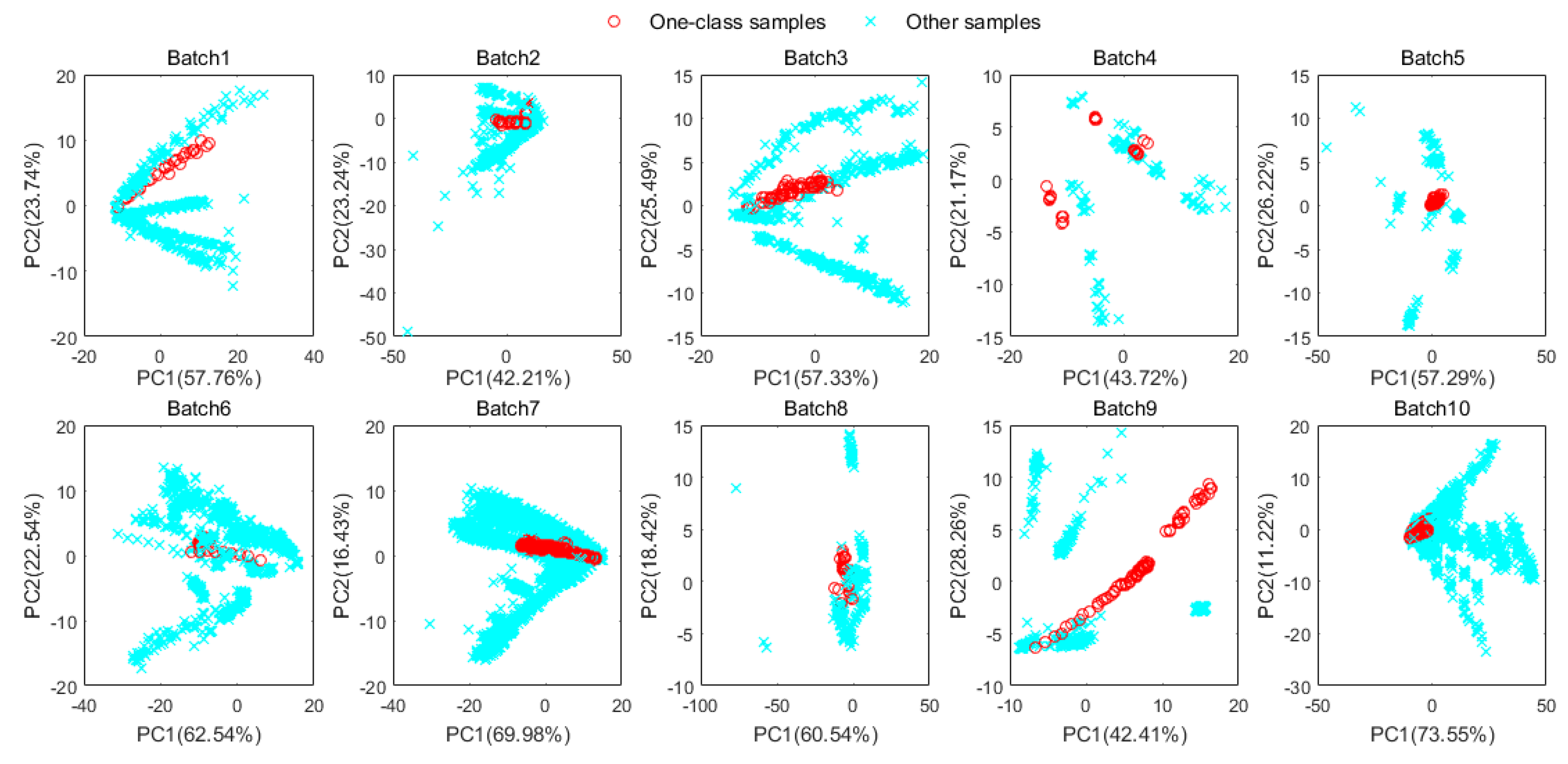
2.1.1. Dataset A
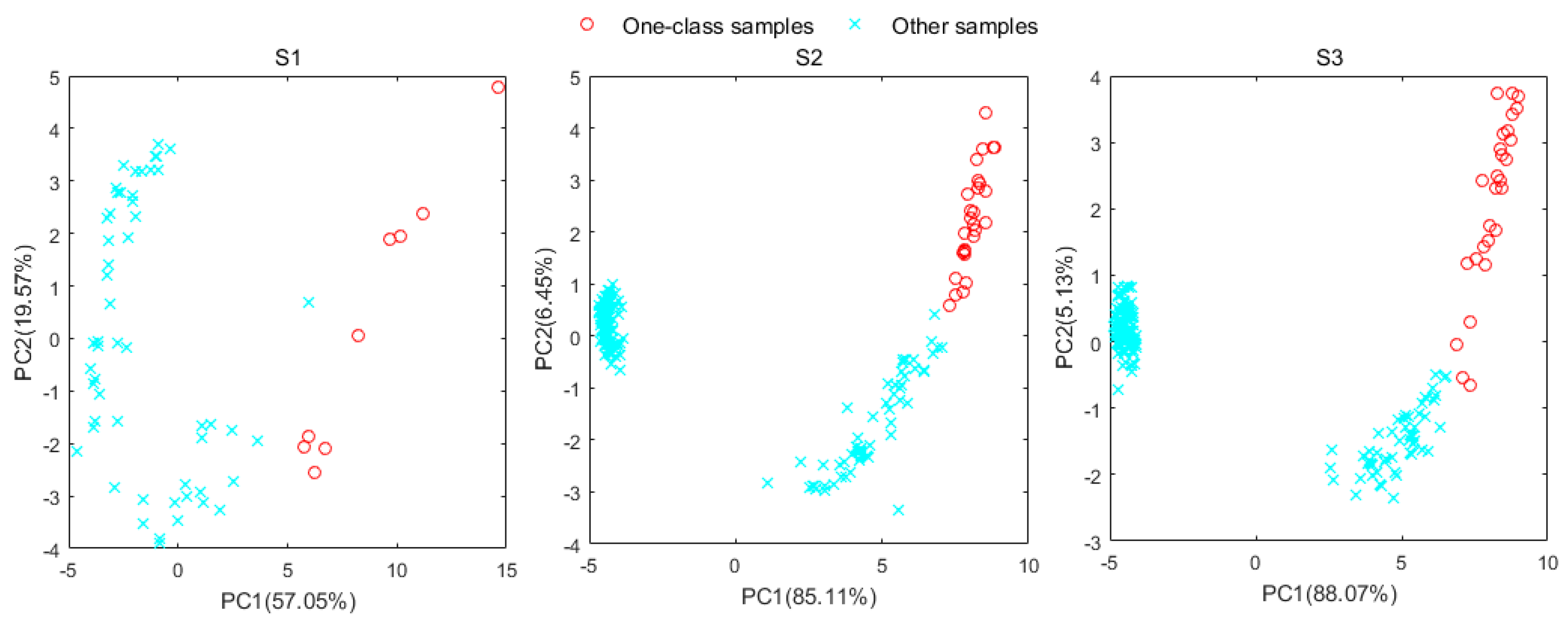
2.1.2. Dataset B
2.2. Notations for Methods
2.3. Transfer-Sample-Based Coupled Task Learning
2.4. Transfer-Sample-Based Multiple Task Learning
2.5. Proposed Methodology
2.5.1. Loss Function Formulation
2.5.2. Solution
3. Results and Discussions
3.1. Validation Settings
3.1.1. Data Arrangement
3.1.2. Parameter Optimization
3.1.3. Reference Methods
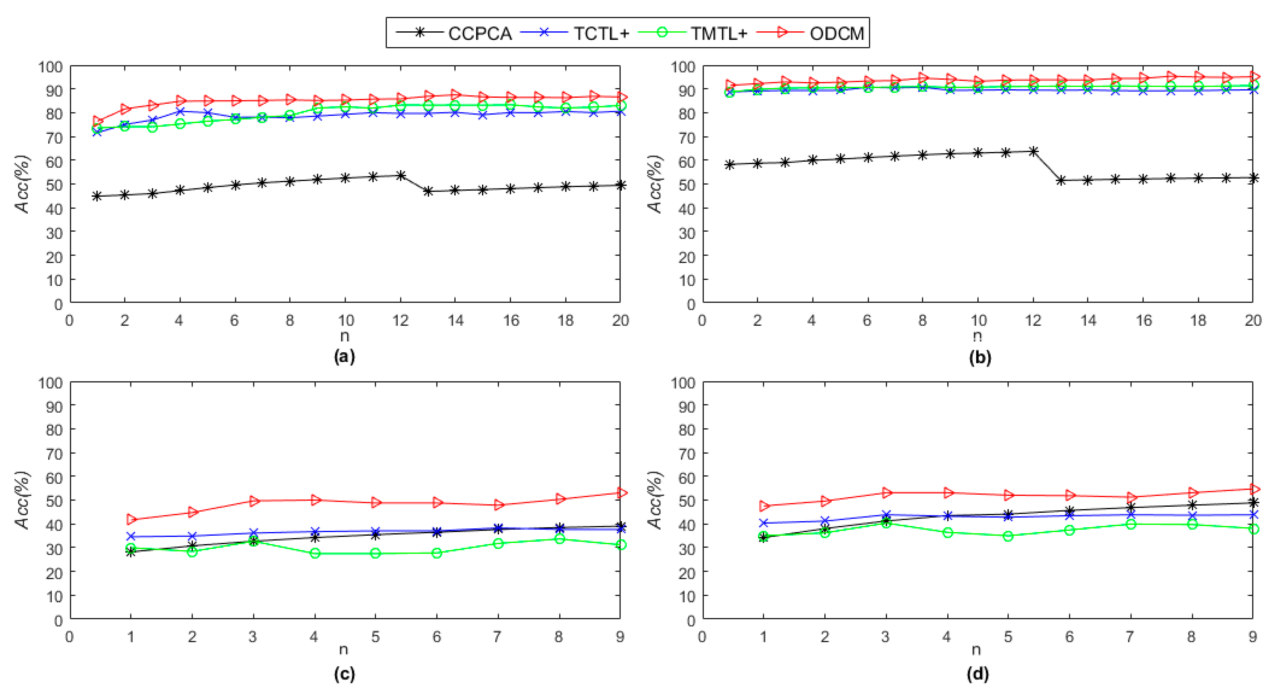
3.2. Recognition Results and Analysis
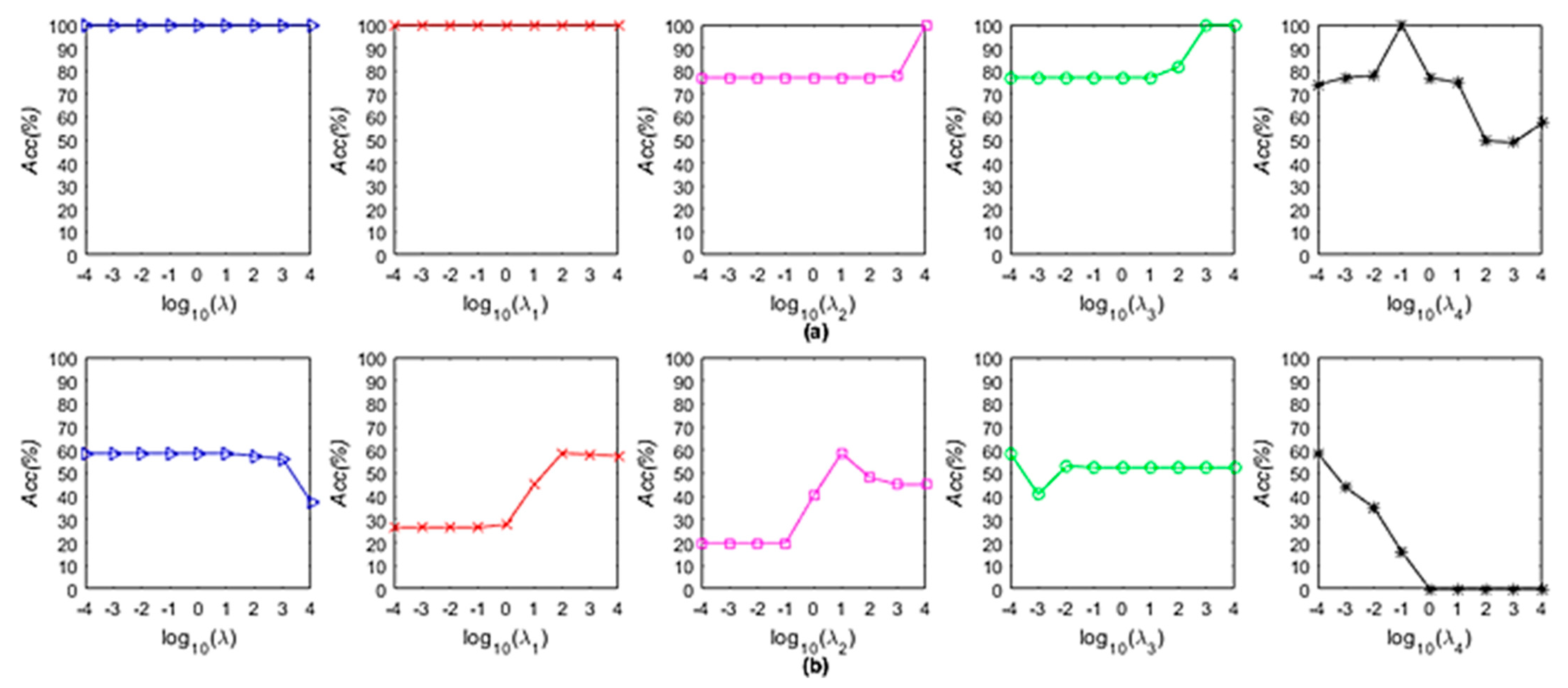
3.3. Parameter Sensitivity Analysis
3.4. Time Complex Analysis
- CPU: Intel I5-8400
- RAM: 8 GB
- Hard disk: 256 GB solid-state drive
- Operation system: Windows 10.
4. Conclusions
Author Contributions
Funding
Institutional Review Board Statement
Informed Consent Statement
Conflicts of Interest
References
- Rusinek, R.; Siger, A.; Gawrysiak-Witulska, M.; Rokosik, E.; Malaga-Toboa, U.; Gancarz, M. Application of an electronic nose for determination of pre-pressing treatment of rapeseed based on the analysis of volatile compounds contained in pressed oil. Int. J. Food Sci. Technol. 2020, 55, 2161–2170. [Google Scholar] [CrossRef]
- Maira, P.A.; Farbod, G.; Lionel, R.; Emmanuel, S.; Emilie, D.; Gaelle, L. Development of Diamond and Silicon MEMS Sensor Arrays with Integrated Readout for Vapor Detection. Sensors 2017, 17, 1163. [Google Scholar]
- Alphus, W. Application of Electronic-Nose Technologies and VOC-Biomarkers for the Noninvasive Early Diagnosis of Gastrointestinal Diseases. Sensors 2018, 18, 2613. [Google Scholar]
- Xu, J.; Liu, K.; Zhang, C. Electronic nose for volatile organic compounds analysis in rice aging. Trends Food Sci. Technol. 2021, 109, 83–93. [Google Scholar] [CrossRef]
- Liang, Z.; Tian, F.; Yang, S.X.; Zhang, C.; Hao, S. Study on Interference Suppression Algorithms for Electronic Noses: A Review. Sensors 2018, 18, 1179. [Google Scholar] [CrossRef] [Green Version]
- Wang, H.; Zhao, Z.; Wang, Z.; Xu, G.; Wang, L. Independent Component Analysis-Based Baseline Drift Interference Suppression of Portable Spectrometer for Optical Electronic Nose of Internet of Things. IEEE Trans. Ind. Inform. 2020, 16, 2698–2706. [Google Scholar] [CrossRef]
- Arunachalam, S.; Izquierdo, R.; Nabki, F. Ionization Gas Sensor Using Suspended Carbon Nanotube Beams. Sensors 2020, 20, 1660. [Google Scholar] [CrossRef] [Green Version]
- Koohsorkhi, J.; Tabatabaei, M.K.; Ghafoorifard, H.; Arough, J.M. High-Performance Immunosensor for Urine Albumin Using Hybrid Architectures of ZnO-Nanowire/Carbon Nanotube. IET Nanobiotechnol. 2019, 14, 126–132. [Google Scholar]
- Chen, Q.; Sun, C.; Ouyang, Q.; Wang, Y.; Liu, A.; Li, H.; Zhao, J. Classification of different varieties of Oolong tea using novel artificial sensing tools and data fusion. LWT Food Sci. Technol. 2015, 60, 781–787. [Google Scholar] [CrossRef]
- Jiang, H.; Xu, W.; Chen, Q. High precision qualitative identification of yeast growth phases using molecular fusion spectra—ScienceDirect. Microchem. J. 2019, 151, 104211. [Google Scholar] [CrossRef]
- Hang, L.; Chu, R.; Jian, R.; Xia, J. Long-term drift compensation algorithms based on the kernel-orthogonal signal correction in electronic nose systems. In Proceedings of the 2015 12th International Conference on Fuzzy Systems and Knowledge Discovery (FSKD), Zhangjiajie, China, 15–17 August 2015. [Google Scholar]
- Padilla, M.; Perera, A.; Montoliu, I.; Chaudry, A.; Persaud, K.; Marco, S. Drift compensation of gas sensor array data by Orthogonal Signal Correction. Chemom. Intell. Lab. Syst. 2010, 99, 28–35. [Google Scholar] [CrossRef]
- Jian, Y.; Lu, K.; Deng, C.; Wen, T.; Jia, Y. Drift Compensation for E-Nose Using QPSO-Based Domain Adaptation Kernel ELM. In International Symposium on Neural Networks; Springer: Cham, Switzerland, 2018. [Google Scholar]
- Yi, R.; Yan, J.; Shi, D.; Tian, Y.; Duan, S. Improving the Performance of Drifted/Shifted Electronic Nose Systems by Cross-Domain Transfer using Common Transfer Samples. Sens. Actuators B Chem. 2020, 329, 129162. [Google Scholar] [CrossRef]
- Liu, T.; Li, D.; Chen, Y.; Wu, M.; Yang, T.; Cao, J. Online Drift Compensation by Adaptive Active Learning on Mixed Kernel for Electronic Noses—ScienceDirect. Sens. Actuators B Chem. 2020, 316, 128065. [Google Scholar] [CrossRef]
- Zhang, L.; Zhang, D. Domain Adaptation Extreme Learning Machines for Drift Compensation in E-nose Systems. IEEE Trans. Instrum. Meas. 2015, 64, 1790–1801. [Google Scholar] [CrossRef] [Green Version]
- Yin, Y.; Wu, W.; Yu, H. Drift elimination method of electronic nose signals based on independent component analysis coupled with wavelet energy threshold value. Nongye Gongcheng Xuebao/Trans. Chin. Soc. Agric. Eng. 2014, 30, 325–331. [Google Scholar]
- Xin, C.; Wang, X.; Huang, Z.; Wang, F. Performance Analysis of ICA in Sensor Array. Sensors 2016, 16, 637. [Google Scholar]
- Perera, A.; Papamichail, N.; BaRsan, N.; Weimar, U.; Marco, S. On-line novelty detection by recursive dynamic principal component analysis and gas sensor arrays under drift conditions. IEEE Sens. J. 2006, 6, 770–783. [Google Scholar] [CrossRef]
- Wu, L.; Lin, A.; Zheng, B.; Pan, J. Study of a signal classification method in energy-saving electronic noses based on PCA and a periodic stochastic resonance. Energy Educ. Sci. Technol. Part A 2013, 31, 385–388. [Google Scholar]
- Zhang, L.; Liu, Y.; He, Z.; Liu, J.; De Ng, P.; Zhou, X. Anti-drift in E-nose: A subspace projection approach with drift reduction. Sens. Actuators B Chem. 2017, 253, 407–417. [Google Scholar] [CrossRef]
- Yi, Z.; Li, C. Anti-drift in electronic nose via dimensionality reduction: A discriminative subspace projection approach. IEEE Access 2018, 7, 170087–170095. [Google Scholar] [CrossRef]
- Liu, T.; Chen, Y.; Li, D.; Yang, T.; Wu, M. Drift Compensation for an Electronic Nose by Adaptive Subspace Learning. IEEE Sens. J. 2019, 20, 337–347. [Google Scholar] [CrossRef]
- Yu, D.; Wang, X.; Liu, H.; Gu, Y. A Multitask Learning Framework for Multi-Property Detection of Wine. IEEE Access 2019, 7, 123151–123157. [Google Scholar] [CrossRef]
- Liu, H.; Li, Q.; Gu, Y. A Multi-task Learning Framework for Gas Detection and Concentration Estimation. Neurocomputing 2020, 416, 28–37. [Google Scholar] [CrossRef]
- Vergara, A.; Vembu, S.; Ayhan, T.; Ryan, M.A.; Homer, M.L.; Huerta, R. Chemical gas sensor drift compensation using classifier ensembles. Sens. Actuators B Chem. 2012, 166–167, 320–329. [Google Scholar] [CrossRef]
- Yan, K.; Zhang, D. Calibration transfer and drift compensation of e-noses via coupled task learning. Sens. Actuators 2016, 225, 288–297. [Google Scholar] [CrossRef]
- Zhang, D.; Guo, D.; Ke, Y. Learning Classification and Regression Models Based on Transfer Samples. In Breath Analysis for Medical Applications; Springer: Singapore, 2017. [Google Scholar]
- Zhang, Y.; Zhou, Z.-H. Multi-Label Dimensionality Reduction via Dependence Maximization. ACM Trans. Knowl. Discov. Data 2010, 4, 1–21. [Google Scholar] [CrossRef]
- Artursson, T.; Eklov, T.; Lundstrom, I.; Mårtensson, P.; Holmberg, M. Drift correction for gas sensors using multivariate methods. J. Chemom. 2015, 14, 711–723. [Google Scholar] [CrossRef]


| Batch ID | Month ID | Number of Samples | Total Number | |||||
|---|---|---|---|---|---|---|---|---|
| Acetone | Acetaldehyde | Ethanol | Ethylene | Ammonia | Toluene | |||
| Batch 1 | Month 1–2 | 90 | 98 | 83 | 30 | 70 | 74 | 544 |
| Batch 2 | Month 3–10 | 164 | 334 | 100 | 109 | 532 | 5 | 1244 |
| Batch 3 | Month 11–13 | 365 | 490 | 216 | 240 | 275 | 0 | 1586 |
| Batch 4 | Month 14–15 | 64 | 43 | 12 | 30 | 12 | 0 | 161 |
| Batch 5 | Month 16 | 28 | 40 | 20 | 46 | 63 | 0 | 197 |
| Batch 6 | Month 17–19 | 514 | 574 | 110 | 29 | 606 | 467 | 2300 |
| Batch 7 | Month 21 | 649 | 662 | 360 | 744 | 630 | 568 | 3613 |
| Batch 8 | Month 22–23 | 30 | 30 | 40 | 33 | 143 | 18 | 294 |
| Batch 9 | Month 24–30 | 61 | 55 | 100 | 75 | 78 | 101 | 470 |
| Batch 10 | Month 36 | 600 | 600 | 600 | 600 | 600 | 600 | 3600 |
| Model | Type | Test Objects | Model | Type | Test Objects |
|---|---|---|---|---|---|
| TGS800 | Metal oxide | Smog | MQ-7B | Metal oxide | Carbon monoxide |
| TGS813 | Methane, ethane, propane | MQ131 | Ozone | ||
| TGS816 | Inflammable gas | MQ135 | Ammonia, sulfide, benzene | ||
| TGS822 | Ethanol | MQ136 | Sulfuretted hydrogen | ||
| TGS2600 | Hydrogen, methane | MP-3B | Ethanol | ||
| TGS2602 | Methylbenzene, ammonia | MP-4 | Methane | ||
| TGS2610 | Inflammable gas | MP-5 | Propane | ||
| TGS2612 | Methane | MP-135 | Air pollutant | ||
| TGS2620 | Ethanol | MP-901 | Cigarettes, ethanol | ||
| TGS2201A | Gasoline exhaust | WSP2110 | Formaldehyde, benzene | ||
| TGS2201B | Carbon monoxide | WSP5110 | Freon | ||
| GSBT11 | Formaldehyde, benzene | SP3-AQ2-01 | Organic compounds | ||
| MQ-2 | Ammonia, sulfide | ME2-CO | Electrochemical | Carbon monoxide | |
| MQ-3B | Ethanol | ME2-CH2O | Formaldehyde | ||
| MQ-4 | Methane | ME2-O2 | Oxygen | ||
| MQ-6 | Liquefied petroleum gas | TGS4161 | Solid electrolyte | Carbon monoxide |
| Scenario | Source Domain | Target Domain |
|---|---|---|
| Setting 1 | Batch i (i = 1, 2, …, K − 1) | Batch (i + 1) |
| Setting 2 | Batch 1 | Batch i (i = 2, …, K) |
| Method | 1–2 | 2–3 | 3–4 | 4–5 | 5–6 | 6–7 | 7–8 | 8–9 | 9–10 | Average |
|---|---|---|---|---|---|---|---|---|---|---|
| CCPCA | 89.95 | 98.68 | 90.68 | 97.97 | 72.91 | 88.54 | 90.48 | 85.96 | 30.69 | 82.87 |
| TCTL | 96.95 | 99.05 | 99.34 | 99.47 | 78.78 | 78.43 | 88.38 | 97.39 | 78.42 | 90.69 |
| TMTL | 97.35 | 98.98 | 99.34 | 99.47 | 78.95 | 97.17 | 95.42 | 96.30 | 71.76 | 92.75 |
| CCPCA+ | 34.11 | 70.73 | 48.13 | 71.43 | 72.68 | 52.85 | 66.79 | 54.16 | 42.34 | 57.02 |
| TCTL+ | 98.15 | 99.05 | 100.00 | 99.34 | 76.22 | 99.44 | 96.55 | 84.30 | 71.87 | 91.66 |
| TMTL+ | 98.94 | 99.63 | 100.00 | 99.34 | 96.00 | 99.37 | 95.40 | 98.99 | 62.21 | 94.43 |
| ODCM | 98.41 | 99.48 | 100.00 | 99.34 | 78.42 | 99.72 | 96.93 | 100.00 | 90.99 | 95.92 |
| Method | 1–2 | 1–3 | 1–4 | 1–5 | 1–6 | 1–7 | 1–8 | 1–9 | 1–10 | Average |
|---|---|---|---|---|---|---|---|---|---|---|
| CCPCA | 89.55 | 82.28 | 59.01 | 60.91 | 63.70 | 38.64 | 22.45 | 45.96 | 35.86 | 55.37 |
| TCTL | 96.95 | 96.85 | 91.30 | 98.98 | 86.78 | 82.51 | 86.05 | 83.19 | 65.75 | 87.60 |
| TMTL | 97.35 | 98.80 | 90.06 | 98.48 | 95.35 | 91.50 | 91.84 | 96.38 | 71.56 | 92.37 |
| CCPCA+ | 34.11 | 61.07 | 55.63 | 46.94 | 58.20 | 46.95 | 22.18 | 24.73 | 38.20 | 43.11 |
| TCTL+ | 98.15 | 98.22 | 98.47 | 94.70 | 69.97 | 75.18 | 78.93 | 67.34 | 80.14 | 84.57 |
| TMTL+ | 98.94 | 99.11 | 98.47 | 93.38 | 78.47 | 71.07 | 80.84 | 77.47 | 75.85 | 85.96 |
| ODCM | 98.41 | 99.26 | 100.00 | 98.68 | 97.21 | 79.16 | 84.67 | 89.37 | 91.33 | 93.12 |
| Method | Setting 1 | Setting 2 | ||||
|---|---|---|---|---|---|---|
| S1–S2 | S2-S3 | Average | S1–S2 | S1–S3 | Average | |
| CCPCA+ | 30.36 | 22.87 | 26.62 | 30.36 | 14.36 | 22.36 |
| TCTL+ | 35.19 | 59.26 | 47.23 | 35.19 | 41.98 | 38.59 |
| TMTL+ | 33.33 | 62.96 | 48.15 | 33.33 | 40.12 | 36.73 |
| ODCM | 49.38 | 61.11 | 55.25 | 49.38 | 58.64 | 54.01 |
| Method | S1–S2 | S1–S3 | S2–S3 | Average |
|---|---|---|---|---|
| CCPCA + SVM | 5.063 | 5.345 | 10.05 | 6.972 |
| TCTL | 0.688 | 0.732 | 0.819 | 0.746 |
| TMTL | 0.706 | 0.681 | 0.651 | 0.679 |
| ODCM | 0.704 | 0.750 | 0.814 | 0.756 |
Publisher’s Note: MDPI stays neutral with regard to jurisdictional claims in published maps and institutional affiliations. |
© 2021 by the authors. Licensee MDPI, Basel, Switzerland. This article is an open access article distributed under the terms and conditions of the Creative Commons Attribution (CC BY) license (https://creativecommons.org/licenses/by/4.0/).
Share and Cite
Zhu, X.; Liu, T.; Chen, J.; Cao, J.; Wang, H. One-Class Drift Compensation for an Electronic Nose. Chemosensors 2021, 9, 208. https://doi.org/10.3390/chemosensors9080208
Zhu X, Liu T, Chen J, Cao J, Wang H. One-Class Drift Compensation for an Electronic Nose. Chemosensors. 2021; 9(8):208. https://doi.org/10.3390/chemosensors9080208
Chicago/Turabian StyleZhu, Xiuxiu, Tao Liu, Jianjun Chen, Jianhua Cao, and Hongjin Wang. 2021. "One-Class Drift Compensation for an Electronic Nose" Chemosensors 9, no. 8: 208. https://doi.org/10.3390/chemosensors9080208
APA StyleZhu, X., Liu, T., Chen, J., Cao, J., & Wang, H. (2021). One-Class Drift Compensation for an Electronic Nose. Chemosensors, 9(8), 208. https://doi.org/10.3390/chemosensors9080208