Abstract
Interpreting chemical analysis results to identify ignitable liquid (IL) residues in fire debris samples is challenging, owing to the complex chemical composition of ILs and the diverse sample matrices. This work investigated a transfer learning approach with convolutional neural networks (CNNs), pre-trained for image recognition, to classify gas chromatography and mass spectrometry (GC/MS) data transformed into scalogram images. A small data set containing neat gasoline samples with diluted concentrations and burned Nylon carpets with varying weights was prepared to retrain six CNNs: GoogLeNet, AlexNet, SqueezeNet, VGG-16, ResNet-50, and Inception-v3. The classification tasks involved two classes: “positive of gasoline” and “negative of gasoline.” The results demonstrated that the CNNs performed very well in predicting the trained class data. When predicting untrained intra-laboratory class data, GoogLeNet had the highest accuracy (0.98 ± 0.01), precision (1.00 ± 0.01), sensitivity (0.97 ± 0.01), and specificity (1.00 ± 0.00). When predicting untrained inter-laboratory class data, GoogLeNet exhibited a sensitivity of 1.00 ± 0.00, while ResNet-50 achieved 0.94 ± 0.01 for neat gasoline. For simulated fire debris samples, both models attained sensitivities of 0.86 ± 0.02 and 0.89 ± 0.02, respectively. The new deep transfer learning approach enables automated pattern recognition in GC/MS data, facilitates high-throughput forensic analysis, and improves consistency in interpretation across various laboratories, making it a valuable tool for fire debris analysis.
1. Introduction
Recent U.S. Fire Administration (USFA) data [1,2] show about a 20% rise in intentional fires in both residential and nonresidential buildings from 2014 to 2023. These fires usually begin with the ignition of items such as trash, paper, and mattresses. A fire history report by the National Fire Protection Association [3] indicates that ignitable liquids (ILs) were responsible for the majority of fatalities (37%), injuries (22%), and direct property losses (19%) in intentional structure fires. The most commonly used ILs are petroleum-based products, such as gasoline, diesel, kerosene, and charcoal lighter fluid, because of their market availability and ease of ignition [4]. Absorbent or porous materials effectively retain ILs because they allow ILs to soak in and be shielded from direct contact with fire, enhancing the IL’s post-fire survivability. Consequently, most fire evidence is collected by directly sampling burned substrates, i.e., fire debris, which contains IL residues [5]. Detecting ILs in fire debris is essential during fire investigations [6], as analyzing these ILs helps identify the fire’s cause—whether accidental or intentional—which is crucial for legal and insurance purposes.
Gas chromatography/mass spectrometry (GC/MS) is considered the gold standard for analyzing the presence of ILs in fire debris samples. The American Society for Testing and Materials International (ASTM International) has established standardized guidelines for identifying residues of ILs in extracts from fire debris samples and classification schemes for assigning the ILs to eight categories using GC/MS, including gasoline, petroleum distillates, isoparaffinic products, aromatic products, naphthenic–paraffinic products, normal alkane products, oxygenated solvents, and miscellaneous [7]. The GC/MS data analysis is mainly based on a visual pattern-matching approach. Typically, an analyst visually compares the patterns of total ion chromatograms (TICs) of unknown samples against those of known reference ILs. Additionally, the extracted ion chromatograms (EICs), i.e., mass chromatograms, are created for the major characteristic ions of each compound type—alkanes, alkenes, aromatics, cycloalkanes, and polynuclear aromatic compounds. Next, the EIC patterns undergo visual evaluation. Identifying major peaks in the EICs and individual target compounds in the TICs is also achieved by comparing their mass spectra with a suitable library and recognizing the relative retention times of compounds in the sample. Thus, interpreting GC/MS data for ILs in fire debris is a complex task. The use of new types of ILs and materials in everyday items further complicates existing IL classification schemes and introduces matrix interferences in the chromatograms [8]. A variety of chemometric tools, including partial least squares discriminant analysis (PLS-DA), hierarchical cluster analysis (HCA), and linear discriminant analysis (LDA), etc., have been developed to facilitate data interpretation and ensure an unbiased process [9]. These tools have been utilized for various purposes, such as classifying ILs based on their brands, grades, or the ASTM classification schemes. Nevertheless, aligning retention times has posed a significant challenge for analyzing GC/MS data in inter-laboratory applications [10]. To address this issue, summed ion mass spectra (i.e., total ion spectra, TIS) were proposed, and this data representation was found to provide sufficient information, enabling the efficient and accurate identification or classification of ILs within a database or library [11,12,13,14,15]. To generate a summed ion mass spectrum, the mass spectrum was averaged across all retention times in the chromatogram [16].
The rapid advancement of deep learning (DL) has transformed and proven highly effective in chemical analysis applications. DL employs computational models for automatic pattern recognition and classification tasks [17]. Its primary distinguishing features from traditional machine learning methods include an architecture comprising multiple interconnected layers and neurons, and its capacity to autonomously identify relevant data features without manual intervention [18]. A convolutional neural network (CNN) is one of the most popular DL models and has demonstrated substantial enhancements in computer vision. The architecture of a CNN comprises several hidden layers, such as convolutional, pooling, and fully connected layers, facilitating the dynamic acquisition of hierarchical data features, ranging from basic to complex levels [19]. CNNs have demonstrated exceptional performance in image classification [20] and are widely used in many fields, such as medical diagnosis [21,22,23,24] and plant disease detection [25,26,27]. Transfer learning is a technique that involves retraining a pre-trained CNN on a smaller data set, mitigating overfitting effects [28] and thus enabling high classification accuracy. The use of CNNs in fire debris analysis remains a relatively new field. For instance, Bogdal et al. transformed 360 GC/MS data into bitmaps and used the images to train an existing CNN to distinguish between samples with and without gasoline residues [29]. Sigman et al. utilized 50,000 in silico-generated fire debris GC/MS data, converting the data into scalograms to train a customized CNN for identifying whether samples contained IL residues [30]. Furthermore, Parl et al. adapted a CNN and used approximately 4000 GC/MS data from actual fire cases to train the CNN for classifying ILs into six categories [31]. A recent study by Sigman et al. utilized 240,000 in silico fire debris sample data to train machine learning models to classify as positive or negative for IL residues [32]. These studies demonstrated the viability of CNNs for analyzing fire debris samples.
In this study, six pre-trained CNNs (GoogLeNet, AlexNet, SqueezeNet, VGG-16, ResNet-50, Inception-v3) were fine-tuned using transfer learning to detect gasoline residues. The testing included not only neat liquids but also simulated fire debris samples, allowing the challenges from the complex chemical compositions of ILs and interference from sample matrices to be addressed in developing this approach. Fewer than 400 GC/MS data of neat gasoline and burned substrate samples were collected using headspace solid-phase microextraction coupled with GC/MS (HS-SPME-GC/MS) to create the training data set. To evaluate the CNNs’ performance after training, two test data sets were prepared: (1) internal laboratory-prepared neat gasoline samples, burned substrate samples, and simulated fire debris samples, and (2) external laboratory-prepared neat gasoline samples, burned substrate samples, and simulated fire debris samples by the National Center for Forensic Science. These data sets aimed to verify the CNNs’ training results, evaluate their ability to predict sample types outside the training distribution, and assess their inter-laboratory applicability. This study highlights the potential of utilizing transfer learning with CNNs to develop a cross-platform classification system, while also discussing the limitations of this approach.
2. Materials and Methods
2.1. Sample Collection and Analysis
2.1.1. Intra-Laboratory Samples
Gasoline samples were collected from five different brands at gas stations in Huntsville, Texas, by our research group in 2022. To prepare stock solutions, 20 mg of each brand of gasoline was dissolved in 1 mL of methanol. Calibrator samples with concentrations ranging from 78 to 10,000 µg/mL were prepared through two-fold serial dilutions of the individual stock solutions. The substrate samples were obtained from Nylon 6,6 carpets with 4 × 4 cm per sample size. Each piece of carpet was ignited using a butane torch (Bernzomatic, Chilton, WI, USA), burned in the air for 1 min, and then allowed to cool to room temperature.
This study involved the analysis of three types of samples using HS-SPME-GC/MS: neat gasoline samples, burned substrate samples, and simulated fire debris samples. Neat gasoline samples were prepared by transferring 5 µL from each calibrator sample into separate 20 mL HS vials (Supelco Inc., Bellefonte, PA, USA). Burned substrate samples were prepared by placing burned carpets of varying weights (50, 150, 250, 350, and 450 mg) into separate 20 mL HS vials. Simulated fire debris samples were prepared by spiking 5 µL of each calibrator sample into 250 mg of burned substrates, also in separate 20 mL HS vials. The extraction was performed using a 23-gauge, 100 μm polydimethylsiloxane (PDMS)-SPME fiber (Supelco Inc., Bellefonte, PA, USA). The resulting extracts were analyzed with an Agilent 7890B gas chromatograph combined with a 5975A mass spectrometer (Agilent Technologies, Santa Clara, CA, USA). The HS-SPME-GC/MS conditions are outlined in Table 1. A total of 405 neat gasoline, 90 burned substrate, and 90 simulated fire debris samples were prepared and analyzed via HS-SPME-GC/MS.

Table 1.
HS-SPME-GC/MS parameters of samples.
2.1.2. Inter-Laboratory Samples
Samples were obtained from the Ignitable Liquids Database and Reference Collection (ILRC) [33], the Substrate Database [34], and the Fire Debris Database [35] provided by the National Center for Forensic Science. The samples in the databases were collected and analyzed by the National Center for Forensic Science at the University of Central Florida, in collaboration with the ILRC committee of fire debris analysts. The databases were developed between 1999 and 2018 [36]. The extraction of all samples utilized activated charcoal strips (Albrayco Technologies Inc., Cromwell, CT) [37] as the medium [38], followed by GC/MS analysis conducted on an Agilent 7890B gas chromatograph combined with a 5977E mass spectrometer (Agilent Technologies, Santa Clara, CA, USA) and an Agilent ALS autosampler G2614A (Agilent Technologies, Santa Clara, CA, USA). The instrument parameters are briefly summarized as follows [34,35,36]: The GC system employed an HP-1 column (or equivalent) with a length of 25 m, an inner diameter of 0.20 mm, and a film thickness of 0.5 microns. Ultra-high-purity helium was used as the carrier gas at a constant flow rate of 0.8 mL/min. Sample injection was carried out with a split ratio of 50:1 and an injection volume of 1 mL, preceded by two pre-injection washes. The injection temperature was maintained at 250 °C. The oven program started at 50 °C with a 3-min hold, then increased at 10 °C per min to 280 °C, which was maintained for 4 min, resulting in a total run time of 30 min. For the MS conditions, the transfer line temperature was maintained at 280 °C. Data acquisition was conducted in scan mode, covering a scan range of 30–350 m/z at a rate of 2–3 scans per s. A solvent delay of 2 min was applied; however, after November 2010, the detector was turned off between 1.54 and 2.00 min instead of applying a traditional delay. A total of 36 GC/MS data of neat gasoline samples, 17 for burned substrate samples and 28 for simulated fire debris samples, were collected. Supplementary Table S1 summarizes the details of each data set.
2.2. Transfer Learning Model Preparation
2.2.1. Data Set Construction
The GC/MS data were divided into “training” and “verification” data sets. The training data set included 390 data from the laboratory-prepared group, comprising 315 GC/MS data of neat gasoline samples and 75 GC/MS data of burned substrate samples. Its purpose was to train existing CNNs for the task investigated in this study. Neat gasoline samples were labeled as “positive of gasoline,” while burned substrate samples were labeled as “negative of gasoline.” In the transfer learning process, the data were randomly split into two parts: 80% for training and 20% for validation. The verification data set comprised 195 intra-laboratory data and 81 inter-laboratory data. This data set aimed to verify the training results and test the CNNs’ prediction performance. Within the verification data, neat gasoline and simulated fire debris samples were deemed to be classified as “positive of gasoline,” whereas burned substrate samples were classified as ”negative of gasoline.” All data mentioned had a ground truth designation indicating the presence or absence of gasoline, following the data analysis method outlined in ASTM E1618-19 [7]. Table 2 presents the details of the GC/MS data sets utilized in this study.
Table 2.
GC/MS data sets used in this study.
2.2.2. GC/MS Data-to-Image Transformation
Before generating images, each GC/MS datum was exported in NetCDF format using the Enhanced ChemStation software (ver. E.01.00.237, Agilent Technologies). The CDF files were utilized to construct data structures that included m/z, abundance values, and retention times through the Bioinformatics Toolbox in the MATLAB environment (ver. R2023a, MathWorks, Natick, MA, USA). The mass signals within the m/z range of 45 to 450 were resampled into 2000 vectors. For further processing, the m/z range of 55 to 156 in the resampled signals and retention times of between 3 and 13 min were selected to retain the characteristic features of gasoline’s GC/MS profile. The abundance of individual m/z values within this specified retention time region was summed to produce the summed ion mass spectrum for each GC/MS datum. These summed ion mass spectra were then transformed into scalograms using the continuous wavelet transform (CWT). The CWT uses inner products to evaluate the similarity between a signal and a family of wavelets that are continuously scaled (stretched or compressed) and shifted in time [39]. It employs a mother wavelet that is dilated and translated to capture features of the signal across both time and scale, producing a detailed two-dimensional time–scale (or time–frequency) representation of a one-dimensional signal [39]. In this work, we compare m/z values and their intensities to time and scale to perform the CWT and generate the scalogram images by using a CWT filter bank [40]. Additional details regarding the CWT are available in our previous report [41].
2.2.3. Transfer Learning with CNNs
In deep transfer learning, CNNs trained on large-scale image data sets—most notably ImageNet—are adapted for new tasks by fine-tuning their weights on a specific data set [42]. This process involves freezing or adding some layers or updating their parameters during training with task-specific data [43]. Such a process reduces the need to train from scratch, lowers data requirements, speeds up convergence, and enhances performance in the target domain [44]. In this study, transfer learning was used to address the limitations of our relatively small (<400 samples) GC/MS-transformed data set. Pretrained CNNs, including GoogLeNet [45], AlexNet [20], SqueezeNet [46], VGG-16 [47], ResNet-50 [48], and Inception-v3 [49], initially designed for classifying images into 1000 categories, were fine-tuned with the proposed scalogram-style chemical data (images derived from CWT of GC/MS data) to distinguish between “gasoline present” and “gasoline absent” patterns. The retraining process of CNNs involved two main steps. First, the network parameters were modified by replacing the final layers. Those layers contained information on integrating the extracted features into class probabilities and labels. For the gasoline classification task, these layers were replaced with a number of filters equal to 2, reflecting the two classes in this study’s data set: “positive of gasoline” and “negative of gasoline.” Additionally, the learning rate factors of the fully connected layer were increased to accelerate learning in the new layers compared to the transferred ones. The second step entailed fine-tuning the network by configuring various training options, including mini-batch size, maximum epochs, initial learning rate, and validation frequency. Basic information such as image input size and number of layers, along with modified network parameters and training options for each pre-trained CNN, is summarized in Table 3. The retraining of the CNNs was executed using the Deep Learning Toolbox under a GPU environment on MATLAB R2023a.
Table 3.
The architecture and fine-tuned parameters of the CNNs used in this study.
2.3. Performance Assessment
Several statistical metrics were employed to evaluate the performance of the CNNs, including accuracy, sensitivity, and specificity. Accuracy is the ratio of the number of correct items to the total number of items, while precision is the number of true positives divided by all predicted positives. Sensitivity, or the true positive rate (TPR), is calculated as the number of true positives divided by the total actual positives. Specificity, or the true negative rate (TNR), is defined as the number of true negatives divided by the total actual negatives. Furthermore, a bootstrapping method was utilized on the intra-laboratory and inter-laboratory data sets to evaluate the performance of the CNNs in this study. This approach enables the estimation of various statistics by repeatedly drawing random samples with replacement from the data set [50]. A total of 100 bootstrap samples were generated from both data sets through this resampling technique. For each bootstrap sample, statistics such as the mean, median, and standard deviation of correctly classified items were calculated. The confidence intervals were constructed by using t-scores multiplied by the standard errors.
3. Results
3.1. Generating Images from GC/MS Data Results
The CWT filter bank addressed in Section 2.2.2 was created to produce the scalograms, employing approximately 12 wavelet bandpass filters per octave (12 voices per octave), with a signal length of 1000 and a sampling frequency of 128. To accommodate the input layer sizes of the CNNs, each scalogram was converted to RGB format and resized to dimensions of 224 by 224 by 3, 227 by 227 by 3, and 299 by 299 by 3, respectively. Figure 1 presents a typical example of a gasoline and burned substrate scalogram.
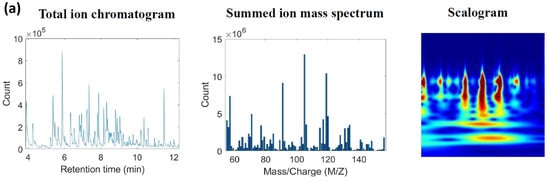
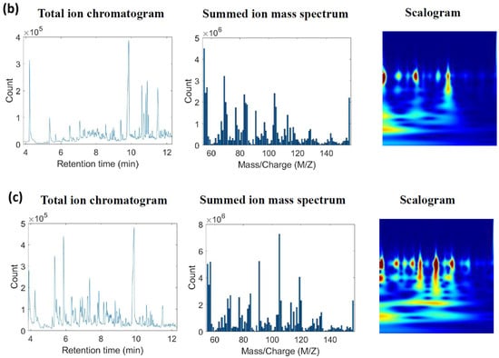
Figure 1.
An example of transformed images from (a) a neat gasoline sample (Brand A, 12.5 μg gasoline/20 mL HS vial); (b) a burned substrate sample (250 mg); (c) a simulated fire debris sample (spiked 12.5 μg Brand A gasoline on 250 mg of burned substrates/20 mL HS vial).
3.2. Training Results
The training progress of the CNNs is depicted in Supplementary Figure S1a–f. The validation accuracy of the CNNs was low at the beginning of the training. However, as they learned the underlying patterns in the transformed images, the validation accuracy showed improvement. As indicated in Table 4, most CNNs achieved their highest validation accuracy without fluctuations between epochs 4 and 6, except for SqueezeNet, which required additional epochs to achieve similar performance. The final validation accuracy for GoogLeNet and Inception-v3 was 98.72% and 91.03%, respectively, while the other CNNs achieved 100% validation accuracy. Generally, the CNNs selected for this study could be retrained to differentiate between samples containing gasoline residues and those without, using the training data prepared in our laboratory. It was also observed that the number of layers and parameters in the CNNs influenced the training duration. More complex CNNs, characterized by a greater number of layers and parameters in their architecture, required longer training times. In this study, VGG-16, ResNet-50, and Inception-v3 necessitated extended training durations because they performed more calculations and adjusted weights and biases throughout the training process.
Table 4.
Training summary of the CNNs.
3.3. Model Performance on Intra-Laboratory Data
To verify the training outcome of the CNNs, different sets of transformed images from neat gasoline and burned substrate samples, prepared in the same manner as those in the training data set, were utilized. These images were regarded as “trained class data” despite not being seen by the CNNs during training. Additionally, to challenge the CNNs’ performance under various conditions, data types that had not been part of the training—specifically, simulated fire debris samples—were introduced. These samples were considered an “untrained class type,” and they had never been seen by the CNNs either. The statistical metrics and bootstrapping results, obtained using the methods described in Section 2.3 for intra-laboratory data verification tests, are summarized in Table 5a–c.
Table 5.
Comparison of the classification performance of the CNNs on the intra-laboratory data.
As shown in Table 5a, nearly every model achieved the highest scores across all measures, meaning that the CNNs were able to distinguish between neat gasoline and burned substrate samples within the “trained class data.” However, Inception-v3 displayed some misclassifications for burned substrate samples, leading to slightly lower accuracy, precision, and specificity. The findings revealed that the CNNs effectively learned the representative features from the images without encountering overfitting issues. In Table 5b, all CNNs showed low accuracy because of their limited sensitivity in predicting simulated fire debris samples (i.e., “untrained class type”). Notwithstanding, their high precision indicated that the CNNs were effective classifiers, as they produced positive results (meaning an unknown sample was correctly identified as a fire debris sample with gasoline residues), with fewer false positive predictions. Therefore, whenever the CNNs predicted a positive outcome, their predictions were more likely to be correct. To investigate the reason for the misclassification of some simulated fire debris samples by the CNNs, Figure 2 illustrates the correct counts classified by each CNN at different concentrations. As noted, all CNNs failed to predict simulated fire debris samples at certain concentrations accurately. To determine the CNNs’ limit of detections (LODs) in this study, an acceptable correct classification rate for each concentration was chosen as 0.6, implying that at least six out of ten simulated fire debris samples should be classified as “positive of gasoline.” Consequently, the LOD of each CNN was determined: 12.5 μg/20 mL HS vial for Inception-v3; 25 μg/20 mL HS vial for GoogLeNet, AlexNet, VGG-16, and ResNet-50; and 50 μg/20 mL HS vial for SqueezeNet. Table 5c presents the classification performance of the CNNs for simulated fire debris samples with concentrations exceeding their respective LODs. Under the circumstances, it was seen that the CNNs exhibited good accuracy, precision, sensitivity, and specificity. This means that the CNNs successfully detected most simulated fire debris samples as positive while identifying burned substrate samples as negative. Among all the CNNs, GoogLeNet outperformed the others in sensitivity, demonstrating a stronger ability to detect unknown samples containing gasoline residues within the simulated fire debris population at concentrations above its LOD. Those findings showed that the CNNs performed exceptionally well at identifying “trained class data,” particularly neat gasoline and burned substrate samples within the intra-laboratory data set. However, they encountered challenges in detecting some “untrained class data” (simulated fire debris samples) within the same data set. The misclassifications of certain simulated fire debris samples resulted from the low concentration of gasoline within the sample matrix. As a result, the CNNs were unable to recognize the characteristics of gasoline compounds, leading to their misclassifications as negative outcomes. Nevertheless, the CNNs still showed promising predictive capabilities for samples with concentrations above the models’ LODs, as shown in Figure 3.
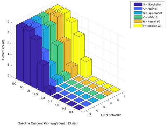
Figure 2.
Comparison of correct counts per concentration obtained from the CNNs for simulated fire debris samples.
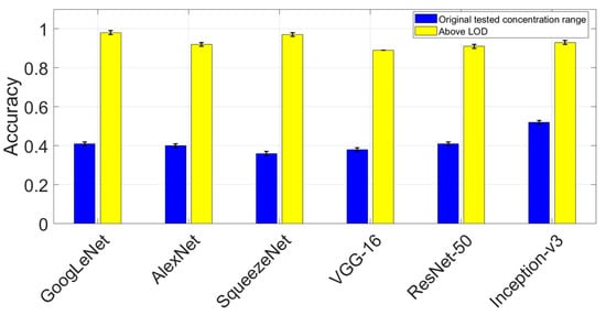
Figure 3.
Comparison of the CNN accuracies between simulated fire debris samples (spiked 1.6–100 μg gasoline on 250 mg of burned substrates/20 mL HS vial) vs. burned substrate samples and simulated fire debris samples (LOD of each CNN) vs. burned substrate samples on the intra-laboratory data.
3.4. Model Performance on Inter-Laboratory Data
The CNNs were further challenged by inter-laboratory data acquired through different extraction methodologies, instruments, GC columns, and instrumental settings. Supplementary Figure S2a–c illustrate examples of TIC comparisons between gasoline samples prepared in-house and those prepared externally. In Supplementary Figure S2a, a neat gasoline sample from the same brand exhibited varying patterns in the GC/MS profiles between our laboratory and an external laboratory. This discrepancy arose from the use of different extraction media for the analytes. The retention times were also shifted due to inconsistencies in column types and GC parameters (such as flow rate, injection temperature, and oven temperature) across different laboratories. Additionally, some data from the external laboratory were obtained from weathered gasoline samples, which may have resulted in a loss of lighter compounds in their composition. Consequently, the GC/MS profile patterns may differ, as illustrated in Supplementary Figure S2b. Furthermore, the external database included neat gasoline data from brands outside the five specific brands used in the training data set, leading to distinct patterns observed in Supplementary Figure S2c. These factors complicated the manual interpretation of inter-laboratory data, making it challenging to identify the presence of gasoline solely through visual pattern comparison of the TICs. The inter-laboratory data set was viewed as another “untrained class type,” and the CNNs had not previously encountered it. In contrast to the “untrained class type” from the intra-laboratory data set (i.e., in-house prepared simulated fire debris samples), the data presented here posed greater challenges for the CNNs for the abovementioned reasons. The same statistical metrics and bootstrapping method described in Section 2.3 were utilized to evaluate the classification performance of the CNNs in analyzing these data. The experimental results are displayed in Table 6a–b.
Table 6.
Comparison of the classification performance of the CNNs on the inter-laboratory data (National Center for Forensic Science database).
Table 6a presents the classification performance of the CNNs in detecting neat gasoline within the inter-laboratory data set. The ResNet-50 exhibited slightly lower sensitivity, while the SqueezeNet demonstrated significantly poorer sensitivity when detecting these challenging samples. The majority of misclassifications by these two CNNs were associated with gasoline samples that had undergone various weathering stages or with samples from brands not included in the training data set. Nevertheless, most CNNs achieved high sensitivity scores, indicating successful detection of all neat gasoline samples analyzed from an external laboratory. The experimental results demonstrated that the ability of these CNNs to learn hierarchical features and share weights enhanced their effectiveness and robustness when analyzing data that differed from their training data set, particularly the data collected from samples with diverse characteristics and under different experimental conditions in an external laboratory. The classification performance of the CNNs were further challenged with simulated fire debris samples from the inter-laboratory data set. Note that these samples were prepared from various stages of weathered gasoline and different substrate materials, contrasting with those in the training data set, which included gasoline diluted at various concentrations and a single substrate type with varying weights. As shown in Table 6b, most CNNs achieved sensitivity scores ranging from approximately 0.80 to 0.90, meaning that 80% to 90% of the simulated fire debris samples were accurately identified. Conversely, AlexNet and VGG-16 demonstrated relatively lower sensitivity. One potential reason for the misclassification of simulated fire debris samples is the influence of specific matrices that contributed signal responses in the mass spectra. The matrices included adhesives, laminate, composite decking, carpet padding, pre-treated wood, vinyl/linoleum, and floor mats or accessories. Most of these materials were used as flooring, building materials, or carpeting, or in automotive applications. The interfering peaks from those matrices dominated the mass spectra, obscuring the peaks representing the gasoline target compounds. As a result, the CNNs could no longer identify the presence of gasoline residues in those samples. Nonetheless, the classification results once more demonstrated the generalization ability of the CNNs to adapt to new and previously unseen data that were not derived from the same distribution as that used during model training. Even with the introduction of more variations in sample types and matrices, most CNNs managed to accurately identify around 80% to 90% of the positive samples. In Table 6a,b, specificity reflects the proportion of burned substrate samples correctly excluded by the CNNs. In particular, GoogLeNet and ResNet-50 achieved specificity scores between 0.70 and 0.76, while the other CNNs produced lower scores, with Inception-v3 scoring only 0.17. The reduced classification accuracy may stem from interference caused by carpet substrates that the CNNs were not trained on. Most of the misclassified substrate samples produced major peaks, including styrene, caprolactam, 2,4,6,8-tetramethyl-1-undecene, and biphenyl, in the mass spectra. The carpet substrates sourced from the National Center for Forensic Science were prepared using various burning methods, including modified destructive distillation, direct, and indirect methods [34]. These methods differ from the one used in our laboratory, as outlined in Section 2.1.1. Additionally, the types of Nylon used at the National Center for Forensic Science may differ from the single type employed in our laboratory. These factors could contribute to the varying mass chromatograms seen in the inter-laboratory data, which posed challenges for the CNNs trained on a relatively simple sample distribution, representing limitations of this study.
4. Discussion
In this study, the retraining of CNNs did not involve manual feature engineering, as the CNNs autonomously recognized and extracted important features from the scalograms transformed from GC/MS data. In the case of gasoline residue detection, the CNNs demonstrated no difficulties in predicting the “trained class data” within the intra-laboratory data set. The parameter settings of all CNN architectures chosen in this study were appropriate for transfer learning, enabling the CNNs to adapt to new tasks, particularly in detecting gasoline residues in neat samples and differentiating these samples from substrate samples, all without the need for human supervision. Quite impressively, the CNNs generalized well, as the models retained their robustness by accurately detecting gasoline residues from “untrained class data,” which consisted of gasoline samples prepared and analyzed under varying experimental conditions. The CNNs’ generalization capability eliminated the necessity for extensive retraining of the models, which may benefit ILs and fire debris analysis. However, the CNNs exhibited some limitations regarding the classifications of certain “untrained class data.” The factor that degraded the classification performance of all the CNNs when analyzing the intra-laboratory data set was the concentration of gasoline in simulated fire debris samples. The lower the gasoline concentration, the poorer the scores observed in the statistical metrics for the CNNs. The solution to this issue was to define the LOD of each CNN. Once the LODs were confirmed, the classifiers could accurately predict unknown fire debris samples whose gasoline concentration exceeded the LOD. Regarding the inter-laboratory data set, the classification performance of the CNNs was subject to stages of weathering of gasoline samples, brands, and substrate types. In this work, the CNNs were trained on neat gasoline samples collected from five brands and one type of burned Nylon 6,6 carpet samples. Therefore, the reasons for the CNNs’ reduced performance could be attributed to the fact that the training data did not represent the variations in samples prepared in an external laboratory. To address this issue, the diversity of or variations in gasoline samples and substrate materials in the training data set may need to be increased.
Based on the experimental outcomes, Inception-v3 achieved the lowest LOD (12.5 μg/20-mL HS vial) with a high level of statistical metrics in predicting the untrained class data in the intra-laboratory data set, followed by GoogLeNet, which achieved the second-lowest LOD (50 μg/20 mL HS vial), with comparable performance, as displayed in Figure 4. GoogLeNet and ResNet-50 performed equally well in predicting the untrained class data in the inter-laboratory data set compared to other CNNs, as shown in Figure 5a,b. Overall, GoogLeNet demonstrated a more balanced classification performance in analyzing the untrained class data in both intra- and inter-laboratory data sets, with an appropriate training time among all the CNNs investigated in this work.
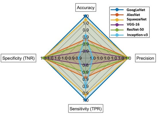
Figure 4.
Comparison of CNN classification performance metrics on simulated fire debris samples (LOD of each CNN) and burned substrate samples in the intra-laboratory data set.
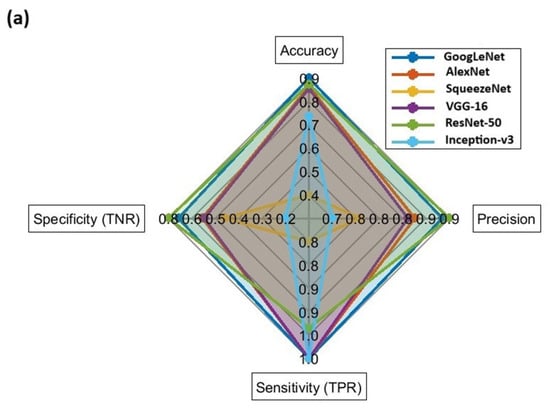
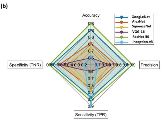
Figure 5.
Comparison of CNN classification performance metrics on (a) neat gasoline samples and burned substrate samples in the inter-laboratory data set; (b) simulated fire debris samples and burned substrate samples in the inter-laboratory data set.
The workflow described in this study—covering data collection, image creation, model selection, and training—offers advantages for analyzing IL residues in fire debris samples. These are complex and lengthy forensic tasks that typically rely on expert analysis of chromatographic data. The workflow can be effectively applied in real forensic settings. Using this method, CNNs can automatically detect patterns in chromatograms or mass spectra that indicate IL presence, eliminating the need for human intervention. Additionally, these models may be incorporated into forensic software, enabling users to upload GC/MS data and receive information such as classification outcomes, confidence scores, and visualizations that highlight key features. Furthermore, once trained, these models can process large data sets efficiently, making them ideal for high-throughput forensic laboratories. They also help minimize variability in manual interpretation, which is vital in legal contexts. Regarding inter-laboratory analysis, this workflow can be trained on data from various laboratories, helping to minimize differences in interpretation and ensure consistent IL classification. As mentioned earlier, forensic laboratories may use different GC/MS instruments or protocols. Nevertheless, the models can adapt to these differences, including retention time shifts and instrument sensitivity, by learning robust features. Consequently, this method allows models to be deployed across laboratories, promoting shared analysis tools and an analyst feedback loop for ongoing enhancement.
5. Conclusions
This study adapted six deep CNNs, pre-trained for image recognition, to classify GC/MS data based on scalograms. The classification task aimed to discriminate between samples containing gasoline residues and those not containing gasoline residues. Based on the training results and performance measures, it is evident that all CNNs were effectively trained to recognize patterns in the scalograms without encountering overfitting issues. The models performed well in predicting trained class data, particularly those involving in-house lab-made neat gasoline and burned substrates. An important finding from the experimental results was the inter-laboratory applicability of the proposed methodologies. The scalograms derived from summed ion mass spectra eliminated the need for retention time alignment in intra-laboratory data. As a result, the CNNs could detect the presence of gasoline residues in data collected from samples with varying attributes (i.e., brands, weathering) and analyses performed under different laboratory conditions (i.e., extraction approach, instrument, and parameters). However, those data were considered untrained class data, meaning that they were outside the training data distribution, which could have impacted the CNNs’ operability. To improve the CNNs’ classification performance, it is recommended to introduce more variations into the training data set, such as different stages of weathering, gasoline brands, and substrate types. Overall, the methodologies presented in this study provided numerous benefits: CNNs autonomously extracted pertinent features from scalograms without the need for manual feature engineering. The retrained CNNs efficiently detected the presence or absence of IL residues in unknown samples, allowing for real-time predictions. Transfer learning reduced the requirement for extensive labeled data sets to train the models effectively, which is particularly advantageous for casework, as many samples are often unavailable at crime scenes. Furthermore, these methods demonstrated the ability to generalize across variations in data collected from different laboratories. In summary, the combination of transfer learning with CNNs and wavelet transformation of GC/MS data could serve as a valuable tool in analyzing IL residues and fire debris samples.
Supplementary Materials
The following supporting information can be downloaded at: https://www.mdpi.com/article/10.3390/chemosensors13090320/s1, Table S1. Information of intra-laboratory samples; Figure S1. The training progress of the CNNs; Figure S2. Comparison of TICs of neat gasoline between lab-made samples and external lab-made samples.
Author Contributions
Conceptualization, T.-Y.H. and J.C.C.Y.; methodology, T.-Y.H. and J.C.C.Y.; software, T.-Y.H.; validation, T.-Y.H.; formal analysis, T.-Y.H.; investigation, T.-Y.H.; resources, T.-Y.H. and J.C.C.Y.; data curation, T.-Y.H.; writing—original draft preparation, T.-Y.H.; writing—review and editing, J.C.C.Y.; visualization, T.-Y.H.; supervision, J.C.C.Y.; project administration, J.C.C.Y.; funding acquisition, T.-Y.H. and J.C.C.Y. All authors have read and agreed to the published version of the manuscript.
Funding
This work was partly funded by the Forensic Sciences Foundation (FSF) Lucas Research Grants: 2022-2023 FSF. The opinions, findings, and conclusions or recommendations expressed in this manuscript are those of the author(s) and do not necessarily reflect those of the FSF.
Institutional Review Board Statement
Not applicable.
Informed Consent Statement
Not applicable.
Data Availability Statement
The raw data supporting the conclusions of this article will be made available by the authors on request.
Acknowledgments
Ting-Yu Huang appreciated the funding support from the Department of Forensic Science, College of Criminal Justice, Sam Houston State University, and the Ministry of Education, Taiwan.
Conflicts of Interest
The authors declare no conflict of interest.
References
- The U.S. Fire Administration (USFA). Residential Fire Estimate Summaries (2014–2023). Available online: https://www.usfa.fema.gov/statistics/residential-fires/intentional.html (accessed on 8 August 2025).
- The U.S. Fire Administration (USFA). Nonresidential Building Intentional Fire Trends (2014–2023). Available online: https://www.usfa.fema.gov/statistics/nonresidential-fires/intentional.html (accessed on 8 August 2025).
- National Fire Protection Association (NFPA). Intentional Structure Fires. Available online: https://www.nfpa.org//-/media/Files/News-and-Research/Fire-statistics-and-reports/US-Fire-Problem/Fire-causes/osintentional.pdf (accessed on 15 March 2025).
- Stauffer, É.; Dolan, J.A.; Newman, R. Flammable and Combustible Liquids; Elsevier: Amsterdam, The Netherlands, 2008; pp. 199–233. [Google Scholar] [CrossRef]
- Stauffer, É.; Dolan, J.A.; Newman, R. Fire debris Analysis; Academic Press: Cambridge, MA, USA, 2008; p. 168. [Google Scholar]
- Almirall, J.R.; Furton, K.G. Analysis and Interpretation of Fire Scene Evidence; CRC Press: Boca Raton, FL, USA, 2004. [Google Scholar] [CrossRef]
- American Society for Testing and Materials (ASTM). Standard Test Method for Ignitable Liquid Residues in Extracts from Fire Debris Samples by Gas Chromatography-Mass Spectrometry. Available online: https://www.astm.org/e1618-19.html (accessed on 15 March 2025).
- Baerncopf, J.; Hutches, K. A review of modern challenges in fire debris analysis. Forensic Sci. Int. 2014, 244, 12–20. [Google Scholar] [CrossRef] [PubMed]
- Martín-Alberca, C.; Ortega-Ojeda, F.E.; García-Ruiz, C. Analytical tools for the analysis of fire debris. A review: 2008–2015. Anal. Chim. Acta. 2016, 928, 1–19. [Google Scholar] [CrossRef]
- Sigman, M.E.; Williams, M.R. Chemometric applications in fire debris analysis. WIREs Forensic Sci. 2020, 2, e1368. [Google Scholar] [CrossRef]
- Misolas, A.A.; Ferreiro-González, M.; Palma, M. Intelligent and automatic characterization of ignitable liquid residues by using total ion spectrum and machine learning. Microchem. J. 2024, 207, 111757. [Google Scholar] [CrossRef]
- Waddell, E.E.; Williams, M.R.; Sigman, M.E. Progress toward the determination of correct classification rates in Fire Debris Analysis II: Utilizing Soft Independent Modeling of Class Analogy (SIMCA). J. Forensic Sci. 2014, 59, 927–935. [Google Scholar] [CrossRef]
- Waddell, E.E.; Song, E.T.; Rinke, C.N.; Williams, M.R.; Sigman, M.E. Progress toward the determination of correct classification rates in fire debris Analysis. J. Forensic Sci. 2013, 58, 887–896. [Google Scholar] [CrossRef]
- Williams, M.R.; Sigman, M.E.; Lewis, J.; Pitan, K.M. Combined target factor analysis and Bayesian soft-classification of interference-contaminated samples: Forensic Fire Debris Analysis. Forensic Sci. Int. 2012, 222, 373–386. [Google Scholar] [CrossRef]
- Sigman, M.E.; Williams, M.R.; Castelbuono, J.A.; Colca, J.G.; Clark, C.D. Ignitable liquid classification and identification using the summed-ion mass spectrum. Instrum. Sci. Technol. 2008, 36, 375–393. [Google Scholar] [CrossRef]
- Waddell, E.E.; Frisch-Daiello, J.L.; Williams, M.R.; Sigman, M.E. Hierarchical cluster analysis of ignitable liquids based on the total ion spectrum. J. Forensic Sci. 2014, 59, 1198–1204. [Google Scholar] [CrossRef]
- Alzubaidi, L.; Zhang, J.; Humaidi, A.J.; Al-Dujaili, A.Q.; Duan, Y.; Al-Shamma, O.; Santamaría, J.; Fadhel, M.A.; Al-Amidie, M.; Farhan, L. Review of deep learning: Concepts, CNN architectures, challenges, applications, future directions. Journal of Big Data. 2021, 8, 53. [Google Scholar] [CrossRef]
- Debus, B.; Parastar, H.; De B Harrington, P.; Kirsanov, D. Deep learning in analytical Chemistry. TrAC Trends Anal. Chem. 2021, 145, 116459. [Google Scholar] [CrossRef]
- Ting, F.F.; Tan, Y.J.; Sim, K.S. Convolutional neural network improvement for breast cancer classification. Expert Syst. Appl. 2019, 120, 103–115. [Google Scholar] [CrossRef]
- Krizhevsky, A.; Sutskever, I.; Hinton, G.E. ImageNet classification with deep convolutional neural networks. Commun. ACM 2017, 60, 84–90. [Google Scholar] [CrossRef]
- Prakash, U.M.; Iniyan, S.; Dutta, A.K.; Alsubai, S.; Ramesh, J.V.N.; Mohanty, S.N.; Dudekula, K.V. Multi-scale feature fusion of deep convolutional neural networks on cancerous tumor detection and classification using biomedical images. Sci. Rep. 2025, 15, 1105. [Google Scholar] [CrossRef]
- Mzoughi, H.; Njeh, I.; BenSlima, M.; Farhat, N.; Mhiri, C. Vision transformers (ViT) and deep convolutional neural network (D-CNN)-based models for MRI brain primary tumors images multi-classification supported by explainable artificial intelligence (XAI). Vis. Comput. 2024, 41, 2123–2142. [Google Scholar] [CrossRef]
- Houssein, E.H.; Abdelkareem, D.A.; Hu, G.; Hameed, M.A.; Ibrahim, I.A.; Younan, M. An effective multiclass skin cancer classification approach based on deep convolutional neural network. Clust. Comput. 2024, 27, 12799–12819. [Google Scholar] [CrossRef]
- Warin, K.; Limprasert, W.; Paipongna, T.; Chaowchuen, S.; Vicharueang, S. Deep convolutional neural network for automatic segmentation and classification of jaw tumors in contrast-enhanced computed tomography images. Int. J. Oral Surg. 2025, 54, 374–382. [Google Scholar] [CrossRef]
- Venkateswara, S.M.; Padmanabhan, J. Deep learning based agricultural pest monitoring and classification. Sci. Rep. 2025, 15, 8684. [Google Scholar] [CrossRef]
- Shafik, W.; Tufail, A.; De Silva, C.L.; Apong, R.H.M. A novel hybrid inception-xception convolutional neural network for efficient plant disease classification and detection. Sci. Rep. 2025, 15, 3936. [Google Scholar] [CrossRef]
- Balasundaram, A.; Sundaresan, P.; Bhavsar, A.; Mattu, M.; Kavitha, M.S.; Shaik, A. Tea leaf disease detection using segment anything model and deep convolutional neural networks. Results Eng. 2024, 25, 103784. [Google Scholar] [CrossRef]
- Huang, Z.; Pan, Z.; Lei, B. Transfer learning with deep convolutional neural network for SAR target classification with limited labeled data. Remote Sens. 2017, 9, 907. [Google Scholar] [CrossRef]
- Bogdal, C.; Schellenberg, R.; Lory, M.; Bovens, M.; Höpli, O. Recognition of gasoline in fire debris using machine learning: Part II, application of a neural network. Forensic Sci. Int. 2022, 332, 111177. [Google Scholar] [CrossRef]
- Akmeemana, A.; Williams, M.R.; Sigman, M.E. Convolutional neural network applications in fire debris classification. Chemosensors 2022, 10, 377. [Google Scholar] [CrossRef]
- Park, C.; Lee, J.; Park, W.; Lee, D. Fire accelerant classification from GC–MS data of suspected arson cases using machine–learning models. Forensic Sci. Int. 2023, 346, 111646. [Google Scholar] [CrossRef] [PubMed]
- Sigman, M.E.; Williams, M.R.; Tang, L.; Booppasiri, S.; Prakash, N. In silico created fire debris data for Machine learning. Forensic Chem. 2024, 42, 100633. [Google Scholar] [CrossRef]
- National Center for Forensic Science. Ignitable Liquids Database. Available online: https://ilrc.ucf.edu/index.php (accessed on 15 March 2025).
- National Center for Forensic Science. Substrate Database. Available online: https://ilrc.ucf.edu/substrate/index.php (accessed on 15 March 2025).
- National Center for Forensic Science. Fire Debris Database. Available online: https://ilrc.ucf.edu/firedebris/index.php (accessed on 15 March 2025).
- National Center for Forensic Science. ILRC-Substrate-Fire Debris. Available online: https://ilrc.ucf.edu/ (accessed on 8 August 2025).
- Sigman, M.E.; Williams, M.R.; Thurn, N.; Wood, T. Validation of ground truth fire debris classification by supervised machine learning. Forensic Chem. 2021, 26, 100358. [Google Scholar] [CrossRef]
- American Society for Testing and Materials (ASTM). Standard Practice for Separation of Ignitable Liquid Residues from Fire Debris Samples by Passive Headspace Concentration with Activated Charcoal. 2019. Available online: https://www.astm.org/e1412-19.html (accessed on 15 March 2025).
- The MathWorks. Continuous Wavelet Transform and Scale-Based Analysis. Available online: https://www.mathworks.com/help/wavelet/gs/continuous-wavelet-transform-and-scale-based-analysis.html (accessed on 8 August 2025).
- The MathWorks. Cwtfilterbank. Available online: https://www.mathworks.com/help/wavelet/ref/cwtfilterbank.html (accessed on 8 August 2025).
- Huang, T.Y.; Yu, J.C.C. Intelligent framework for cannabis classification using visualization of gas chromatography/mass spectrometry data and transfer learning. Front. Anal. Sci. 2023, 3, 1125049. [Google Scholar] [CrossRef]
- Kim, H.E.; Cosa-Linan, A.; Santhanam, N.; Jannesari, M.; Maros, M.E.; Ganslandt, T. Transfer learning for medical image classification: A literature review. BMC Med. Imaging 2022, 22, 69. [Google Scholar] [CrossRef]
- Iman, M.; Arabnia, H.R.; Rasheed, K. A review of deep transfer learning and recent advancements. Technologies 2023, 11, 40. [Google Scholar] [CrossRef]
- Zhao, Z.; Lian, F.; Jiang, Y. Recognition of rice species based on gas chromatography-ion mobility spectrometry and deep learning. Agriculture 2024, 14, 1552. [Google Scholar] [CrossRef]
- Szegedy, C.; Liu, W.; Jia, Y.; Sermanet, P.; Reed, S.; Anguelov, D.; Erhan, D.; Vanhoucke, V.; Rabinovich, A. Going deeper with convolutions. In Proceedings of the 2015 IEEE Conference on Computer Vision and Pattern Recognition (CVPR), Boston, MA, USA, 7–12 June 2015. [Google Scholar]
- Iandola, F.; Han, S.; Moskewicz, M.W.; Ashraf, K.; Dally, W.J.; Keutzer, K. SqueezeNet: AlexNet-level accuracy with 50x fewer parameters and <0.5 MB model size. arXiv 2016, arXiv:1602.07360. [Google Scholar]
- Simonyan, K.; Zisserman, A. Very deep convolutional networks for large-scale image recognition. In Proceedings of the 3rd International Conference on Learning Representations (ICLR 2015), San Diego, CA, USA, 7–9 May 2015. [Google Scholar]
- He, K.; Zhang, X.; Ren, S.; Sun, J. Deep residual learning for image recognition. In Proceedings of the 2016 IEEE Conference on Computer Vision and Pattern Recognition, Las Vegas, NV, USA, 26 June–1 July 2016. [Google Scholar]
- Szegedy, C.; Vanhoucke, V.; Ioffe, S.; Shlens, J.; Wojna, Z. Rethinking the Inception architecture for computer vision. arXiv 2016, arXiv:1512.00567. [Google Scholar]
- Egbert, J.; Plonsky, L. Bootstrapping Techniques; Springer: Berlin, Germany, 2020; pp. 593–610. [Google Scholar]


Disclaimer/Publisher’s Note: The statements, opinions and data contained in all publications are solely those of the individual author(s) and contributor(s) and not of MDPI and/or the editor(s). MDPI and/or the editor(s) disclaim responsibility for any injury to people or property resulting from any ideas, methods, instructions or products referred to in the content. |
© 2025 by the authors. Licensee MDPI, Basel, Switzerland. This article is an open access article distributed under the terms and conditions of the Creative Commons Attribution (CC BY) license (https://creativecommons.org/licenses/by/4.0/).