Integrating Sensor Data, Laboratory Analysis, and Computer Vision in Machine Learning-Driven E-Nose Systems for Predicting Tomato Shelf Life

Abstract

Assessing the quality of fresh produce is essential to ensure a safe and satisfactory product. Methods to monitor the quality of fresh produce exist; however, they are often expensive, time-consuming, and sometimes require the destruction of the sample. Electronic Nose (E-Nose) technology has been established to track the ripeness, spoilage, and quality of fresh produce. Our study developed a freshness monitoring system for tomatoes, combining E-Nose technology with storage condition monitoring, color analysis, and weight-loss tracking. Different post-purchase scenarios were investigated, focusing on the influence of temperature and mechanical damage on shelf life. Support Vector Classifier (SVC) and k-Nearest Neighbor (kNN) were applied to classify storage scenarios and storage days, while Support Vector Regression (SVR) and kNN regression were used for predicting storage days. By using a data fusion approach with Linear Discriminant Analysis (LDA), the SVC achieved an accuracy of 72.91% in predicting storage days and an accuracy of 86.73% in distinguishing between storage scenarios. The kNN yielded the best regression results, with a Mean Absolute Error (MAE) of 0.841 days and a coefficient of determination of 0.867. The results highlight the method’s potential to predict storage scenarios and storage days, providing insight into the product’s remaining shelf life.

1. Introduction

The 2021 UNEP Food Waste Index Report states that in 2019, 931 million tonnes of food waste were generated globally, totaling 17% of the global food production [1]. A large portion of this waste is generated at the household level, contributing roughly 61% of all food waste in the product chain [1]. Consumers often rely on “best-before” and “use-by” dates to determine the shelf life of food. The Regulation (EU) No 1169/2011 defines and regulates such labeling in the EU. However, this exempts fresh fruits and vegetables from using “best-before” and “use-by” date labeling [2]. Therefore, identifying suitable storage conditions and estimating the remaining shelf life introduces a challenge for consumers.

The Oxford English Dictionary defines shelf life as “The length of time that a commodity may be stored without becoming unfit for use or consumption” [3]. In the case of food, this includes the time during which the food is safe for consumption and retains the expected properties and nutritional values [4]. According to Schmidt et al. [5], fruits and vegetables account for the highest food waste in private households. This observation aligns with the finding that food is primarily discarded due to durability concerns, which accounts for 57.6% of the reported reasons for disposal [5].

For fruits and vegetables, the expected properties mostly consist of a desirable appearance, flavor, and texture. The factors influencing fruit and vegetable shelf life differ from those of other foods because, unlike processed foods, they consist of living tissue until consumed. The duration for which they retain their desirable properties depends on the biochemical (e.g., chlorophyll degradation and enzymatic browning), physical (e.g., mechanical damage and chilling injury), microbiological (e.g., fungal infection), and environmental influences (e.g., temperature and humidity) [6]. Therefore, frequent checks along the product chain are required, mostly during production, storage, and retail. Such checks often consist of expensive, time-consuming, and/or destructive measurements (e.g., gas chromatography, texture analyzer, and titration) [6]. Non-destructive tests can be carried out as an alternative to destructive measurements, and the remaining shelf life can be predicted. These techniques include, for example, near-infrared spectroscopy, X-ray scattering, and machine vision [6]. Another promising method to monitor shelf life involves the detection of volatile compounds using Electronic Nose (E-Nose) technology [7]. The resulting multi-dimensional data can be effectively analyzed using machine learning algorithms [8]. The aroma of fruits and vegetables is a key quality attribute that changes over time. Aroma changes measured using E-Nose technology can indicate the ripening stage and provide insights into their shelf life [9,10,11,12]. For instance, off-odors caused by fungal or bacterial infections can signal spoilage. These infections are often associated with prior improper handling, which causes mechanical damage to the tissue and compromises the natural barrier against pathogens [6].

Despite the well-established, non-destructively measured shelf life indicators such as aroma, color, appearance, storage temperature, and humidity, their practical monitoring and interpretation remain limited in real-world settings. Especially retail employees and consumers lack effective tools to accurately assess the condition of food products or determine their remaining shelf life. Additionally, storage conditions, particularly temperature and humidity during transportation, can directly impact the remaining shelf life of fruits and vegetables. However, retailers often lack access to data verifying whether the conditions have been maintained in the previous steps in the supply chain. This highlights the importance of developing rapid, easy-to-use tools for evaluating the remaining shelf life of fruits and vegetables. Such tools can enhance decision-making processes at the retail stage and improve consumers’ trust and safety. Hence, within this work, we (i) developed a sensor-based, non-destructive E-Nose system to monitor tomato freshness after purchase, (ii) applied a data fusion approach combining aroma profiles, color, weight, and storage condition data with machine learning techniques to enhance predictive performance, and (iii) investigated the effects of temperature and mechanical damage on the remaining shelf life of tomatoes.

The tomatoes in our study were grouped in different post-purchase storage scenarios and stored for 14 days. During storage, we measured Volatile Organic Compounds (VOCs) with an E-Nose system, the color of the fruit over time using RGB images and computer vision, the percentual weight loss, and the storage conditions (temperature and humidity) of each scenario. The recorded data was later processed and analyzed using machine learning algorithms to classify and predict the tomatoes’ storage day and respective storage scenarios. Using a data fusion approach, we aim to track tomato early spoilage and reveal differences in different storage scenarios at the household level that can influence shelf life. Our objective is to evaluate whether our proposed system can accurately predict the remaining shelf life under typical consumer storage conditions despite their unknown pre-purchase history. By focusing on consumer-relevant quality indicators, such as the absence of visible damage or spoilage, this approach aims to classify tomatoes over a defined storage period.

The remainder of this work is structured as follows: Section 2 provides a detailed description of this study’s materials and applied methods. Subsequently, Section 3 presents the key findings derived from the data analysis. Afterward, in Section 4, these results are discussed, including limitations and threats to validity. Finally, Section 5 concludes the findings of the paper.

2. Materials and Methods

This section details the methodologies employed in our study, providing a comprehensive overview of our experimental approach, data processing, and machine learning technologies.

2.1. Sample Selection and Storage Scenarios

Tomatoes (Solanum lycopersicum) were purchased from a German grocery store to mimic typical consumer purchasing conditions. The tomatoes were chosen to be of similar size (7–8 cm diameter), ripeness (red ripe state), and without visible damage to obtain comparable samples. Only tomatoes with attached panicles were chosen. Before starting the trial, the panicle was cut, leaving only a small piece attached to each tomato. Since the samples were freshly purchased and not stored under controlled conditions prior to the experiment, the day of purchase is subsequently labeled as T₀. Different storage scenarios were simulated by storing the tomatoes at a cooled temperature of 11 °C (cooled temperature, Label: T_c) in a cooling system (Klarstein Shiraz Duo 29, Chal-Tec GmbH Berlin, Germany) and at ambient conditions (room temperature 19 °C, Label: T_rt). The influence of mechanical damage on shelf life was tested by dropping some tomatoes from a height of 80 cm to simulate a drop from a table to create randomized pressure marks. All damaged tomatoes were stored at ambient conditions (room temperature damaged, Label: T_rtd).

The storage conditions (temperature and relative humidity) were continuously monitored. Three randomly selected tomatoes from each storage scenario were measured thrice a week to collect weight loss, color, and E-Nose data. The sampled tomatoes were discarded after the measurements to ensure independent samples. Additionally, three tomatoes from each storage scenario were measured throughout the storage period to observe how shelf life influences the E-Nose signals. While storage conditions refer to the measured environmental parameters such as temperature and humidity, storage scenarios represent the predefined experimental groups used as labels for the tomatoes, combining specific condition settings and factors like mechanical damage. In the following sections, the procedure for each measurement will be explained in detail.

2.2. Storage Condition Monitoring

Understanding the impact of storage conditions on shelf life is crucial and requires constant monitoring of the environment. Therefore, a temperature and humidity sensor (ASAIR DHT 22/AM2302, Guangzhou, China) was placed in the cooling system and next to the tomatoes stored at room temperature. The data was collected over a storage period of 14 days using an Arduino microcontroller (Arduino Uno Rev 3, Monza, Italy). Due to strong fluctuations in the sensor signal, the raw data was filtered to remove outliers. Values exceeding 1.5 times the interquartile range (IQR) below the first quartile or above the third quartile were identified as outliers and removed from the dataset. For each measurement day, daily averages were calculated for all monitored storage variables, incorporating the 24-h sensor recordings, and were assigned to the samples measured that day.

2.3. Weight Loss

Weight loss due to water loss through transpiration can cause fruits to lose key quality attributes consumers value, such as firmness and freshness, which may lead to their disposal. Factors like cuticle structure, gas permeability, and surrounding temperature determine the rate of water loss [13]. The amount of weight loss was estimated by weighing the tomatoes on the day of purchase (m_initial) and the respective measurement day (m_current) using a PCB 350-3 laboratory scale (Kern & Sohn GmbH, Balingen, Germany). The extent of water lost from the fruit by transpiration is assumed to be far larger than losses from, e.g., lost volatiles. Therefore, we treated the measured weight loss entirely due to water loss. Weight loss was calculated as a percentage of the original weight to account for different fruit sizes and weights (see Equation (1)).

$$Weightloss={\displaystyle \frac{m_{current}}{m_{initial}}}\ast 100$$

(1)

2.4. Color Analysis

Color is an important metric for the determination of fruit ripeness and freshness. For the color analysis, the tomatoes were photographed from three sides (bottom, left, right) using a digital camera (Sony 7 E-Mount, Tokyo, Japan) inside an enclosed photo box. The tomatoes in the pictures were recognized using Autodistill’s Grounded Segment Anything Model (SAM) (IDEA-Research, Shenzen, China) with the prompt “Tomato”. The segmented images were converted to the CIELAB color space. The average L*, a*, and b* color values were calculated for each picture. The final color value of each tomato was calculated as the average of the color values detected in the three pictures. ChatGPT 4o was employed to assist interpreting trends within the color data.

2.5. E-Nose

This subsection provides a detailed overview of the E-Nose system used in this study, including a description of the system and the measurement procedure.

2.5.1. The E-Nose System

The E-Nose sensor array comprises 12 commercially available metal oxide semiconductor (MOS) sensors.

Table 1. Sensor types and target gases of the MOS sensors used in the E-Nose system.

Sensor Type	Target Gas
MQ2 *	Methane, Butane, LPG, Smoke
MQ3 *	Ethanol, Smoke
MQ4 *	Methane, CNG
MQ5 *	Natural Gas, LPG
MQ6 *	LPG, Butane
MQ8 *	Hydrogen
MQ9 *	Carbon Monoxide, flammable Gasses
MQ135 *	Ammonia, Nitrous Oxides, Benzene, CO2
MQ136 **	Hydrogen Sulfide
MQ137 **	Ammonia
MQ138 **	Toluene, Alcohol, Acetone, Hydrogen

* Hanwei Electronics Co., Ltd., Zhengzhou, China, ** Winsen Electronics Technology Co., Ltd, Zhengzhou, China.

shows the sensor types, distributors, and target gases. The sensors were connected to an Arduino microcontroller (Arduino Mega 2560 Rev 3, 154 Monza, Italy), which was used for data collection.

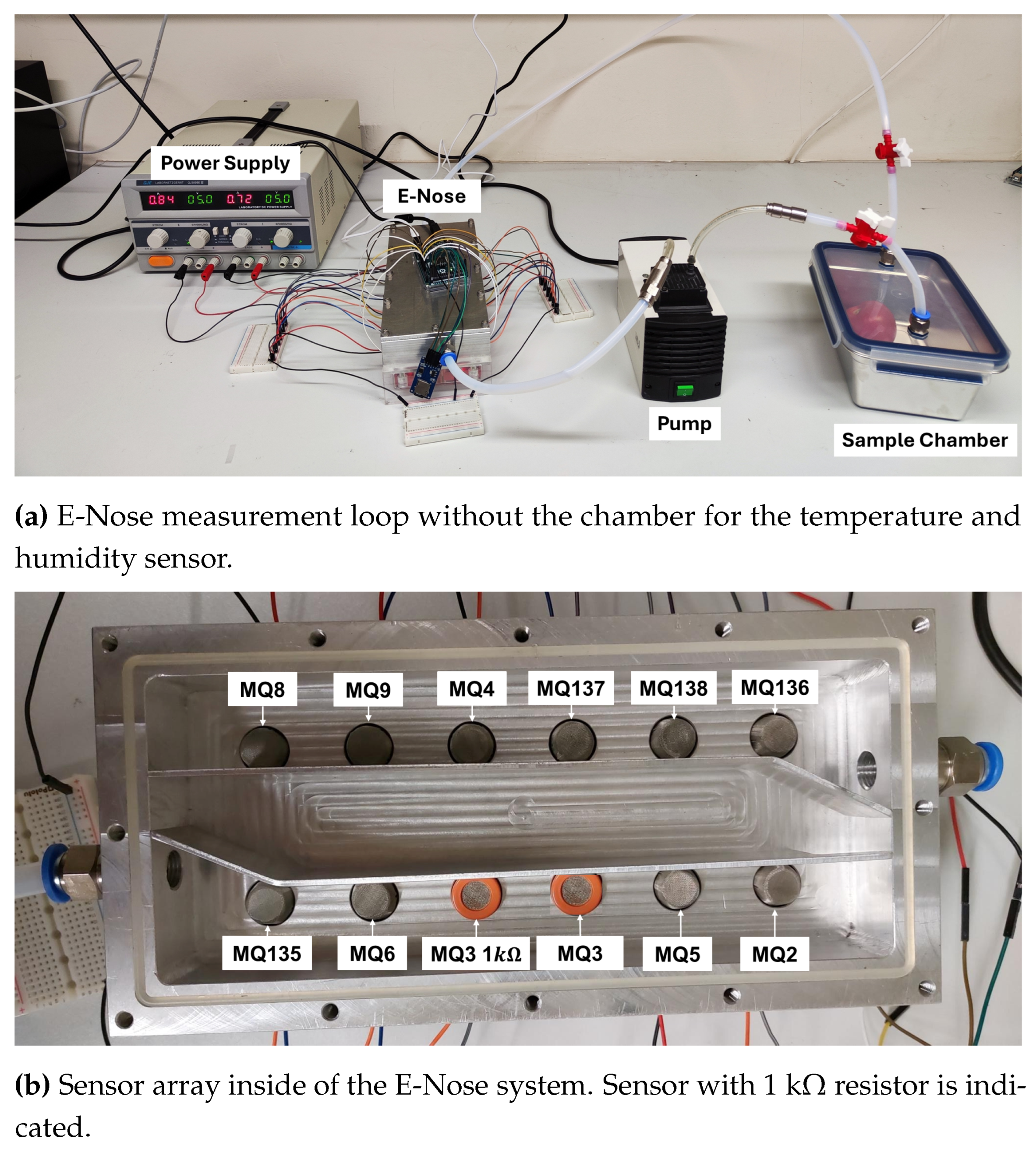
The collected data was retrieved using an SD-Card module. The system setup is depicted in Figure 1a. An external power unit (Komerci QJ3005EIII, Ebern, Germany) was implemented to supply the sensors’ heating elements. The E-Nose system includes three chambers connected by tubes. Polytetrafluoroethylene (PTFE) tubes and a metal chamber were employed to avoid odor attachment. Further, the system was built airtight to avoid sample leakage or contamination. Airflow was produced using a pump (N 811 KN.18, KNF, Freiburg i.B., Germany) with a fixed flow rate of 11.5 L/min. Two three-way valves and one two-way valve were utilized to direct the airflow during the measurement phases. Inside the E-Nose (Figure 1b), the 12 gas sensors were placed in two rows with even spacing. Eleven of the twelve sensors contained a resistor of 10 kΩ. In Figure 1b, the sensor with a 1 kΩ resistor is indicated. The airflow inside the E-Nose was directed in an S-shape using aluminum deflector plates to ensure the sample air passed each sensor. The sample chamber and the temperature and humidity sensor chamber were made of 2 L stainless steel boxes. Temperature and humidity inside the E-Nose were monitored using an independent Arduino (Arduino Nano, Monza, Italy) connected to a DHT22 temperature humidity sensor (ASAIR DHT 22/AM2302, Guangzhou, China).

Due to the complex mixture of VOCs in the tomato odor profile and the non-specificity of the gas sensors, no exact concentrations of individual substances were measured. Instead, the change in sensor resistance was used as a quantitative measure of the gas concentration present in the sample. During measurements, the sensor resistance of all sensors was recorded with a frequency of 1 Hz.

2.5.2. Measurement Procedure

The E-Nose measurement procedure was divided into three phases. In the first phase, the sample was enriched for 15 minutes to accumulate a sufficient concentration of VOCs for the measurement. During this phase, the baseline resistance of the E-Nose in fresh air was recorded. The second phase involved pumping the sample gas through the sensor circuit for 5 minutes until the sensor readings stabilized at a constant level. In the final phase, the sensors were regenerated with fresh air for 5 minutes to ensure complete recovery of the sensors.

2.6. Machine Learning Pipeline

The following subsection outlines the machine learning pipeline, including the E-Nose data processing, feature pre-processing steps and the algorithms used for model development. ChatGPT 4o and 3.5 were employed to support the coding process. The data used in this pipeline is available at https://doi.org/10.5281/zenodo.15469472 (accessed on 9 July 2025).

2.6.1. E-Nose Data Processing

The E-Nose measurements were analyzed using Python 3.11. For each sensor, the ratio of resistance, as surrogates for the gas concentration, in the sample air to fresh air (R_S/R₀) was derived from the E-Nose recordings. This normalization minimized the influence of ambient conditions on the measurement results.

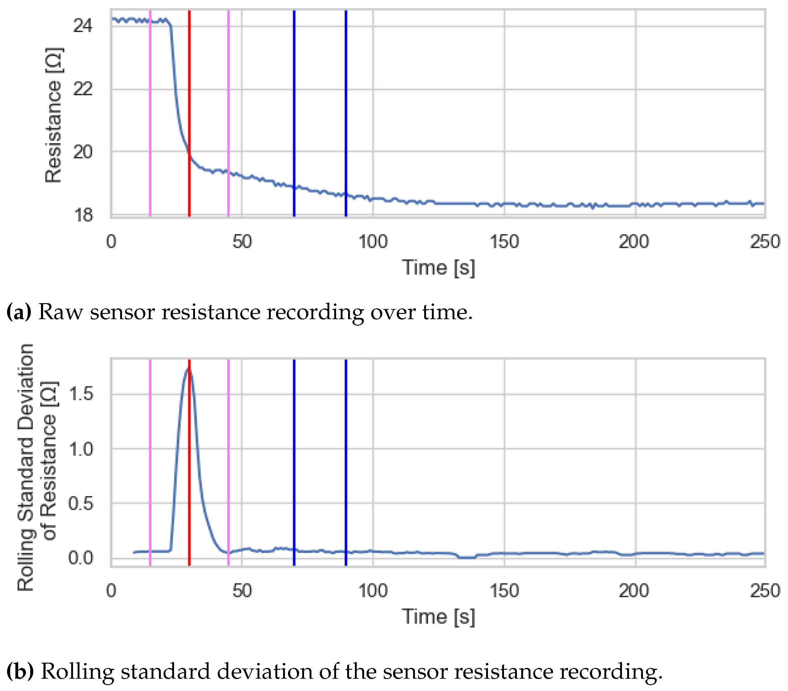
As the target gas was introduced manually, its point of addition had to be identified in the data individually. Therefore, breakpoint detection was employed. After introducing the target gas, the sensor resistance sharply declined, followed by stabilization at a lower level (see Figure 2a).

The exact time of this change was determined by analyzing the rolling standard deviation of the sensor signal (see Figure 2b). The breakpoints were identified by computing the rolling standard deviation of the data with a right-aligned window size of 10 s. The red line (Figure 2b) marks the maximum rolling standard deviation and represents the right boundary of the sensor’s adaptation phase. It indicates the point at which the sensor array has adjusted to the presence of the sample gas. The left boundary (pink line) corresponds to the initial rise in signal variability, occurring approximately 15 s earlier, and marks the beginning of the sample gas introduction. Therefore, all sensor readings up until 15 s (pink line) were included in the calculation of R₀. R_S was calculated by averaging the sensor readings between 40 and 60 s (blue lines) after the breakpoint, allowing slow and gradual signal changes to be captured. Due to strongly fluctuating sensor signals, all breakpoints were compared with the corresponding breakpoint of the MQ3 sensor, which reliably detected the gas addition. Any deviation exceeding 10 s was considered a false detection, and the breakpoint was replaced with the MQ3 reference breakpoint.

The ratio was adjusted based on each tomato’s weight on the day of measurement (m_current). Weight normalization was applied to account for varying weight of the individual tomatoes, to reduce bias from size-related signal strength, given that all samples were measured using the same procedure. The weight-normalized Sensor Ratio Response (SRR_w) was calculated as shown in Equation (2).

$$SR{R}_w={\displaystyle \frac{\left(\frac{R_S}{R_0}\right)}{m_{current}}}$$

(2)

2.6.2. Feature Pre-Processing

Samples measured on the day of purchase (T₀) were excluded from dataset, as they represent the same tomatoes across all storage scenarios. For the analysis, all observations with missing values were removed. Furthermore, one measurement with no recorded data was manually removed. In total 52 tomato samples were included in the further processing steps. Dimensionality reduction and visualization of data separability were performed using two established techniques: Principal Component Analysis (PCA) and Linear Discriminant Analysis (LDA). Both techniques were applied to three distinct datasets: the first included only SRR_w values (12 features and 52 observations), the second comprised storage monitoring parameters, weight data, and color analysis (SWC; 6 features and 52 observations), and the third combined the features from both datasets (Combined; 18 features and 52 observations). All three datasets additionally included the storage scenario and the storage day. Either storage scenario or storage day was used as the target variable, while the other one was not considered in the model.

Depending on the data distribution, the separability of the samples based on the first two PC/LD scores was examined using either ANOVA followed by a Tukey post-hoc test or a Kruskal–Wallis test followed by Dunn’s test. The results of the statistical tests are available on Zenodo https://doi.org/10.5281/zenodo.15469472 (accessed on 9 July 2025). However, PCA failed to provide clear data separation for all three datasets. Therefore, it was excluded from this study as a pre-processing method. Five-fold cross-validation splitting the datasets (SRR_w, SWC, and Combined) into training and test sets (80:20) was applied to evaluate the performance of the models. All features were normalized to a mean of $\mu =0$ and standard deviation $\sigma =1$ to ensure that all variables lie within the same range and are not weighted differently due to different scales. For the classification tasks, normalization, dimensionality reduction, and model training were performed within the five-fold cross-validation pipeline. StratifiedKFold cross-validation was used to ensure that class distributions were preserved across folds. For the regression tasks, dimensionality reduction was applied to the respective datasets prior to splitting them into training and test sets for model training. Afterward, the normalization and model training were performed within the five-fold cross-validation pipeline. If no dimensionality reduction was applied, only normalization and model training within the cross-validation were performed.

2.6.3. Machine Learning Models

A Support Vector Classifier (SVC) and a k-Nearest Neighbor (kNN) classification algorithm were implemented to classify the storage day and the storage scenario. Accuracy, precision, recall, and F1 score were selected as performance metrics for the classification models. A Support Vector Regression (SVR) with a linear kernel and a kNN regressor algorithm were applied to predict the storage day. Mean Average Error (MAE), Mean Square Error (MSE), and the coefficient of determination (R²) were selected as performance metrics. For the model training and evaluation, a five-fold cross-validation approach was selected as described in Section 2.6.2. Performance measures were calculated as the average over the five folds. The machine learning algorithms were applied using their default parameter settings.

3. Results

This section presents the study’s results. First, the outcomes of the storage monitoring, weight loss tracking, and color analysis are reported, followed by the findings from the E-Nose measurements. Subsequently, the components of the machine learning pipeline are outlined, and the performance of the applied machine learning algorithms are evaluated. Only results that will be discussed in Section 4 are displayed.

3.1. Storage Condition Monitoring

Section 2.1 describes the three storage scenarios. For each setting, the temperature and relative humidity were tracked. For T_rt and T_rtd, the temperature averaged $18.84\pm 1.10$ °C and $18.70\pm 0.80$ °C. The corresponding relative humidity values were $41.25\pm 4.53$% for T_rt and $42.73\pm 4.23$% for T_rtd. In the T_c scenario, the temperature showed a mean value of $11.18\pm 1.64$ °C with a relative humidity of $49.49\pm 9.61$%.

3.2. Weight Loss

Figure 3 presents the daily average measurement from the three randomly selected tomatoes per storage scenario. The remaining weight, expressed as a percentage, illustrates the weight loss over time. While all tomatoes lost weight, the extent varied across the storage scenarios. After 14 days, tomatoes stored in the T_c scenario experienced less weight loss than tomatoes stored in the other storage scenarios. Damaged tomatoes (T_rtd) exhibited greater weight loss than undamaged tomatoes (T_rt).

3.3. Color Analysis

Color values in the CIELAB color space were obtained from daily photographs by segmenting the tomato pixels using the Grounded SAM model with the prompt “Tomato”, followed by color space conversion and averaging of the masked pixel values. Tomato detection was successful; however, the segmentation sometimes captured unintended elements, such as the metal ring used to position the tomatoes or the panicles attached to the sample. Including non-red tomato parts and other objects in the image mask could lead to errors in detecting the correct color value. The tomato’s color development over the 14-day storage period was quantified using the CIELAB color space parameters L*, a*, and b*. An overview of the average color values of the three randomly selected tomatoes per measurement day and scenario is provided in

Table 2. Calculated mean CIELAB values and standard deviation of the tomatoes over the 14 days storage period. T₀: day of purchase; T_c: cooled temperature; T_rt: room temperature; T_rtd: room temperature damaged.

Storage Day	Storage Scenarios	L*	a*	b*
0	T0	38.81 ± 1.58	45.36 ± 0.60	35.90 ± 0.85
3	Tc	40.48 ± 1.78	43.11 ± 2.58	36.10 ± 1.71
5	Tc	36.23 ± 1.23	42.43 ± 0.98	32.53 ± 1.13
7	Tc	39.68 ± 2.00	46.22 ± 0.91	37.18 ± 1.32
10	Tc	38.49 ± 0.74	45.84 ± 1.29	35.51 ± 1.52
12	Tc	39.94 ± 1.19	44.85 ± 1.07	35.88 ± 0.82
14	Tc	40.45 ± 2.15	45.86 ± 0.62	36.35 ± 0.45
3	Trt	39.98 ± 1.11	45.11 ± 0.90	36.08 ± 1.43
5	Trt	36.98 ± 0.90	41.93 ± 1.35	32.45 ± 1.32
7	Trt	36.66 ± 0.61	44.25 ± 0.78	33.22 ± 0.25
10	Trt	36.03 ± 0.44	43.75 ± 0.70	32.38 ± 0.41
12	Trt	37.17 ± nan	43.37 ± nan	32.65 ± nan
14	Trt	38.99 ± 2.57	46.05 ± 3.25	35.95 ± 3.18
3	Trtd	38.33 ± 1.30	45.51 ± 1.79	34.52 ± 2.43
5	Trtd	36.22 ± 1.26	43.04 ± 2.88	31.97 ± 2.94
7	Trtd	36.07 ± 0.31	41.53 ± 1.89	30.31 ± 2.25
10	Trtd	37.11 ± 0.80	40.75 ± 0.93	30.36 ± 1.20
12	Trtd	37.82 ± 1.41	43.89 ± 2.01	33.59 ± 1.30
14	Trtd	37.92 ± 2.18	44.79 ± 2.62	32.85 ± 2.45

. For each tomato, three pictures were used as described in Section 2.4, to calculate the respective value. Measurements taken on the day of purchase (T₀) were used as a reference for comparison.

L* values showed minor fluctuations over time across all storage scenarios. Relatively stable L* values were observed for T_c with final values of 40.45 ± 2.15. T_rt displayed a temporary decrease between days 5 and 10, with recovery by the end of the storage period. In comparison, a decrease was observed in the T_rtd scenario until day 7 (36.07 ± 0.37), followed by an increase to 37.92 ± 2.18 by the end of storage. In the T_c scenario, a* only slightly increased from the initial value to day 14 (45.86 ± 0.62). The a* value for T_rt peaked at the end of the storage period at 46.05 ± 3.25 (day 14). T_rtd depicted a decline until day 10 (40.75 ± 0.93), with a slight increase afterward. b* values in the T_c scenario depicted a drop on day 5 (32.53 ± 1.13), increasing to a similar value at the storage end in comparison to the starting point. In the T_rt scenarios a decrease compared to the starting point was indicated for day 5, 7, 10, and 12 with an increase at the last storage day (35.98 ± 3.18). The most pronounced decrease was observed under T_rtd, with b* dropping from 34.52 ± 2.43 on day 3 to 30.36 ± 1.20 on day 10, followed by a slight increase at the end.

3.4. E-Nose

The temperature inside the E-Nose system ranged from 21 °C to 23 °C, while the relative humidity fluctuated between 30 and 60%. From the raw data, the breakpoints and SRR_w values were calculated. Figure 4 displays the SRR_w mean values of 4 sensors (MQ135, MQ136, MQ137, and MQ3) for the continuously monitored tomatoes in the different storage scenarios. The T_c scenario deviates from the other two storage scenarios for the displayed sensors. Notably, T_rt shows a decrease in SRR_w values after day 10 for the sensors MQ136 and MQ137, and a drop from day 6 for MQ3. Visual inspection revealed that one of the continuously monitored tomatoes stored under the T_rt scenario exhibited signs of microbial spoilage toward the end of the trial. For SRR_w values of the randomly sampled tomatoes, the variance within each storage scenario was too high to allow a clear visual grouping.

3.5. Machine Learning Pipeline

This section presents the results related to the machine learning pipeline, including the dimensionality reduction and the performance of the classification and regression models.

3.5.1. Dimensionality Reduction

We applied the supervised LDA method for dimensionality reduction. It searches for the hyperplane that maximizes separability between classes while minimizing the variance within the classes of the target variable. Class separation was evaluated by comparing the mean values of LD1 and LD2 using either ANOVA followed by a Tukey post-hoc test or Kruskal–Wallis tests followed by Dunn’s test, depending on the data distribution and the homogenity of variances of the features.

As mentioned in Section 2.1, samples measured on the day of purchase (T₀) were excluded from the LDA analysis to avoid introducing identical data into multiple classes. The LDAs shown in Figure 5, Figure 6 and Figure 7 were conducted on the full datasets of the three cases, SRR_w, SWC, and Combined, to enable visual comparison.

For all three datasets (SRR_w, SWC, and Combined), a total of 2 LDs were calculated for the storage scenario and 5 LDs for the storage days. The 2 LDs for the storage scenario contained 100% of the variance between the classes. For the storage days, the first 2 LDs contained over 80% of the variance. Figure 5 shows plots of the first two LDs calculated using the SRR_w values. The class separation results show that LD1 could distinguish the storage scenarios T_rt from T_rtd and T_c, while LD2 could separate T_rtd from T_c. Significant differences between storage days were observed for all comparisons except between storage days 5 and 12 and storage days 7 and 10. To further explore trends within the data, LDA plots were color-coded by storage day and symbol-coded by storage scenario, allowing a visual assessment of patterns. This approach revealed that, for the SRR_w dataset, no consistent grouping was possible.

In Figure 6, the LDA performed on the SWC dataset is displayed. The evaluation of the class separation revealed that LD1 could distinguish the storage scenarios T_c from T_rt and T_rtd, while LD2 could separate all three scenarios. Storage days also differed significantly, except between storage days 7 and 10 as well as 12 and 14. Using the SWC dataset, a visual grouping of the storage days within each storage scenario (Figure 6 (left)) becomes more evident. While some overlap remains during the initial days, clearer separation between the days can be observed toward the end of the storage period across all three scenarios. In contrast, when using storage day as the target variable (Figure 6 (right)), the LDA only partially reveals separable groupings of the storage scenarios within each day.

The third LDA was performed with the combined dataset (Figure 7). The analysis of the class separation confirmed the same group separations among storage scenarios as observed in the LDA performed with the SWC dataset. Furthermore, all storage days showed significant differences in LD1 or LD2 scores. The combined dataset demonstrated an enhanced ability to visually distinguish storage days within each storage scenario compared to the previous datasets. While grouping storage scenarios within individual days was still only partially successful, the overall class separation appeared more distinct, indicating better performance of the LDA in this case.

LDA was not applied as a classification model because the required assumptions of normality and equal covariance matrices, verified through Shapiro-Wilk and Bartlett’s test, were not consistently met. Instead, LDA was only used for dimensionality reduction as a pre-processing step within the pipeline, and other models were employed for the classification.

3.5.2. Classification Models

Four performance metrics—accuracy, precision, recall, and the F1 score—were calculated for each model to determine the quality of the classification.

Table 3. Table of performance metrics determined for the SVC and kNN models, averaged over five-fold cross-validation. A separate model was performed for each combination of pre-processing steps, input features, and classified variables. Storage day and storage scenario were classified. The grey rows indicate the best performing models for the storage day and storage scenario classification.

Algorithm	Pre-Processing	Input Features	Target Variable	Accuracy	Precision	Recall	F1 Score
SVC	None	SRRw	Day	0.324 ± 0.117	0.259 ± 0.108	0.283 ± 0.113	0.243 ± 0.101
SVC	None	SWC	Day	0.482 ± 0.172	0.455 ± 0.244	0.483 ± 0.178	0.435 ± 0.191
SVC	None	Combined	Day	0.422 ± 0.069	0.399 ± 0.150	0.433 ± 0.097	0.389 ± 0.113
SVC	LDA	SRRw	Day	0.651 ± 0.106	0.611 ± 0.084	0.650 ± 0.062	0.597 ± 0.075
SVC	LDA	SWC	Day	0.655 ± 0.151	0.597 ± 0.155	0.650 ± 0.133	0.597 ± 0.141
SVC	LDA	Combined	Day	0.729 ± 0.113	0.683 ± 0.078	0.717 ± 0.085	0.672 ± 0.082
SVC	None	SRRw	Scenario	0.289 ± 0.159	0.181 ± 0.124	0.300 ± 0.166	0.220 ± 0.141
SVC	None	SWC	Scenario	0.811 ± 0.077	0.832 ± 0.092	0.811 ± 0.075	0.803 ± 0.079
SVC	None	Combined	Scenario	0.598 ± 0.081	0.596 ± 0.145	0.600 ± 0.100	0.568 ± 0.090
SVC	LDA	SRRw	Scenario	0.505 ± 0.132	0.517 ± 0.196	0.506 ± 0.128	0.484 ± 0.148
SVC	LDA	SWC	Scenario	0.851 ± 0.107	0.859 ± 0.115	0.850 ± 0.111	0.846 ± 0.113
SVC	LDA	Combined	Scenario	0.867 ± 0.094	0.872 ± 0.097	0.872 ± 0.097	0.866 ± 0.098
kNN	None	SRRw	Day	0.265 ± 0.080	0.247 ± 0.080	0.250 ± 0.075	0.222 ± 0.056
kNN	None	SWC	Day	0.465 ± 0.091	0.415 ± 0.052	0.467 ± 0.085	0.407 ± 0.052
kNN	None	Combined	Day	0.362 ± 0.114	0.327 ± 0.168	0.333 ± 0.139	0.306 ± 0.150
kNN	LDA	SRRw	Day	0.673 ± 0.079	0.628 ± 0.096	0.667 ± 0.053	0.621 ± 0.063
kNN	LDA	SWC	Day	0.520 ± 0.102	0.444 ± 0.146	0.500 ± 0.091	0.438 ± 0.120
kNN	LDA	Combined	Day	0.729 ± 0.078	0.694 ± 0.035	0.717 ± 0.041	0.669 ± 0.042
kNN	None	SRRw	Scenario	0.251 ± 0.096	0.210 ± 0.138	0.272 ± 0.113	0.201 ± 0.091
kNN	None	SWC	Scenario	0.795 ± 0.141	0.788 ± 0.177	0.789 ± 0.162	0.778 ± 0.165
kNN	None	Combined	Scenario	0.675 ± 0.091	0.717 ± 0.113	0.678 ± 0.099	0.671 ± 0.096
kNN	LDA	SRRw	Scenario	0.480 ± 0.102	0.500 ± 0.126	0.489 ± 0.102	0.474 ± 0.097
kNN	LDA	SWC	Scenario	0.851 ± 0.137	0.844 ± 0.146	0.844 ± 0.146	0.844 ± 0.146
kNN	LDA	Combined	Scenario	0.867 ± 0.094	0.872 ± 0.097	0.872 ± 0.097	0.866 ± 0.098

shows the calculated metrics for the SVC and kNN models, with the grey rows indicating the best-performing models for the storage days and storage scenarios. The results generally reveal the following trends: Using LDA as a pre-processing step showed the best results across all target variables.

The best-performing model to classify the storage day used the combined dataset with LDA as the pre-processing step and SVC as the classification algorithm (accuracy = 0.729, precision = 0.683, recall = 0.717, F1 score = 0.672). For the storage scenario classification, the highest accuracy was achieved using the combined dataset with LDA and SVC (accuracy = 0.867, precision = 0.872, recall = 0.872, F1 score = 0.866) or kNN with the same configuration (accuracy = 0.867, precision = 0.872, recall = 0.872, f1 score = 0.866). Generally, the models trained with the SRR_w dataset exhibited the lowest performance for both target variables and classification algorithms for most cases.

3.5.3. Regression Models

Models were trained exclusively for the number of days in storage. SVR with a linear kernel and kNN regression were employed as regression models. The same datasets and pre-processing steps used for the classification models were also applied to the regression models. The target variable for the LDA was the storage day.

Table 4. Table of performance metrics determined for the SVR and kNN regression models to predict the storage day, averaged over five-fold cross-validation. The grey row indicates the best performing model.

Algorithm	Pre-Processing	Input Features	MAE	MSE	R2
SVR	None	SRRw	3.977 ± 0.410	19.204 ± 2.534	−0.525  ± 0.375
SVR	None	SWC	2.217 ± 0.334	8.161 ± 2.060	0.302 ± 0.358
SVR	None	Combined	2.084 ± 0.331	7.391 ± 2.862	0.374 ± 0.325
SVR	LDA	SRRw	1.793 ± 0.445	5.364 ± 2.235	0.528 ± 0.284
SVR	LDA	SWC	2.226 ± 0.364	8.092 ± 2.516	0.284 ± 0.402
SVR	LDA	Combined	1.087 ± 0.286	1.707 ± 0.702	0.865 ± 0.049
kNN	None	SRRw	4.011 ± 0.671	20.829 ± 5.807	−0.566 ± 0.214
kNN	None	SWC	2.540 ± 0.661	9.161 ± 3.868	0.350 ± 0.079
kNN	None	Combined	3.396 ± 0.583	15.497 ± 3.946	−0.173 ± 0.175
kNN	LDA	SRRw	1.780 ± 0.384	5.933 ± 1.510	0.500 ± 0.209
kNN	LDA	SWC	2.423 ± 0.485	9.435 ± 3.850	0.290 ± 0.274
kNN	LDA	Combined	0.841 ± 0.201	1.458 ± 0.744	0.867 ± 0.110

shows the regressions’ MAE, MSE, and the R² values, with the grey row indicating the best-performing model.

The SRR_w models without pre-processing showed negative coefficients of determination, indicating poor predictive performance. Applying LDA to separate the storage days before the regression improved the model performance. The models trained on the combined dataset with LDA as a pre-processing step achieved the best results. For the kNN model, an MAE of 0.841, an MSE of 1.458, and a coefficient of determination (R²) of 0.867 were achieved. The SVR model also showed a low MAE at 1.087; however, the MSE was slightly higher at 1.707, and the R² was marginally lower at 0.865.

4. Discussion

This section discusses the study’s key findings, including the E-Nose system and measurement procedure, the applied storage scenarios, and their impact on shelf life, with particular attention to the influence of temperature and mechanical damage. Furthermore, the machine learning pipeline is evaluated, focusing on dimensionality reduction, classification, and regression approaches. Finally, potential threats to validity are discussed.

4.1. E-Nose

The functionality and data quality of the developed E-Nose system were evaluated, focusing on measurement accuracy. Inert materials such as aluminum and PTFE were used in the construction to reduce the risk of contamination. However, since the experiments were conducted in a non-controlled environment without regulated temperature, humidity, or air quality, external factors can not be excluded, as they may have caused variations in the measured values. Comparisons of the baseline resistances (R₀) revealed variations across measurement days and individual samples. Similar patterns have been reported in literature, where strong differences in the sensor resistance of MOS sensors and shifts in signal ranges between measurements were observed [14]. One possible cause can be insufficient sensor regeneration during the measurement, while another potential source of interference is the condition of the fresh air. Laboratory activities and cleaning agents used near the E-Nose system can increase the concentration of VOCs in the fresh air. To avoid contaminated fresh air, Chou et al. [15] used an improvised air filter consisting of activated carbon in a metal tube to purify the air of organic compounds before gas enrichment. Furthermore, the temperature and humidity of the fresh air influence the sensor signal [16]. Kislev et al. [14] report that even differences in the weather and the ventilation of the laboratory room can lead to strong fluctuations in the measurement signal, largely due to differences in temperature and humidity. In addition, Tang et al. [17] used a water vapor generator to control the humidity. However, since a higher humidity leads to lower sensor sensitivity, drying the air is preferred over enriching it with moisture [9]. Since the humidity values within the E-Nose system varied between 30 to 60% (see Section 3.4) controlling this parameter could improve the consistency and comparability of the measurements. Synthetic air could be an alternative to filtering the fresh air as it offers controlled conditions, minimizing environmental variability [12].

Therefore, implementing a filter system for the fresh air supply should be considered in future improvements as it would enhance the system’s reliability in non-controlled environments, enabling practical use, for example, at the retail stage.

The measurements in this study were conducted within a closed gas circuit. Each measurement lasted approximately 5 min, allowing sufficient time to achieve a stable measurement state, even for gases present in high concentrations. The observed decrease in signal strength may result from a reduction of the target gas concentration caused by the sensors’ combustion of the target gases during measurement. The more likely cause of the decrease in signal strength is the sample’s dilution due to the volume of the E-Nose system. Closed measuring circuits [9,18] and open measuring circuits [15,17] have been used for E-Nose applications before. Brezmes et al. [18] used a sensor chamber with a volume of 1 L for their closed setup compared to the sample chamber, which had a volume of 5 L. Chen et al. [9] also used a sample chamber volume of 5 L compared to a sensor chamber of 0.015 L. In comparison, the sample chamber in this study had a volume of 2 L, and the sensor chamber had a volume of 0.594 L. Additionally, the chamber containing the temperature and humidity sensor contributed another 2 L. This relatively large overall system volume, combined with a higher proportion of clean air to sample air, may have led to dilution effects, reducing the VOC signal strength even in closed measuring circuits. For the open-circuit E-Nose systems, sample and measurement chambers of similar volumes are often used, as no mixing of the samples is expected because the sample is discarded after measurement [15,17]. The pump’s flow rate (11.5 L/min) was higher than the values for E-Nose systems reported in the literature. Usual pumping rates in E-Nose systems are between 0.8 L/min [15] and 2 L/min [17,18]. The comparatively high flow rate in the closed system may entail challenges due to the dilution of the sample air, which reduces the concentration of VOCs over time. Additionally, a high flow rate reduces the residence time of highly concentrated VOCs within the E-Nose, and when combined with the dilution effect, this results in an overall weakening of the signal strength. Future improvements to the E-Nose system should include a larger sample chamber and a pump with a lower flow rate to reduce dilution effects.

At the beginning of the measurement, the sensor’s baseline remains stable. Following the addition of the target gas, a rapid decrease in sensor resistance is observed (see Figure 2a). Once an equilibrium between oxygen binding and consumption at the sensor surface is reached, the resistance stabilizes. The observed pattern aligns with resistance and conductivity behaviors reported in the literature [9,10,12,15,18]. The magnitude of the decrease and the rate of change differed depending on the sensor, which was expected due to the different target gases and individual sensor differences. Continuous fluctuations observed in several sensor signals may be attributed to the low resolution of the analog-to-digital converter integrated into the Arduino. The Arduino Mega 2560 Rev3 is based on the ATmega 2560/V microprocessor, which is equipped with a 10-bit analog-to-digital converter [19]. The Arduino can measure voltages between 0 and 5 volts, which results in a minimum resolution of 0.0049 V with 1024 measuring steps (10 bits). When the actual measured voltage falls between two steps, fluctuations in the signal can occur. In the literature, analog-to-digital converters with an input range of 13 bits [9] to 24 bits [15] are used, corresponding to a signal resolution up to 16,384 times more accurate. Improving the overall signal quality will require integrating an analog-to-digital converter with higher resolution into the E-Nose system.

4.2. Influence of Temperature and Mechanical Damage on Shelf Life

Post-harvest losses are often caused by decay, external damage, and harvesting at improper maturity stages [20]. Additionally, tomatoes are climacteric and chilling-sensitive fruit, which makes them easily affected by storage conditions. Ripe tomatoes can be stored at around 10 °C without experiencing chilling injuries [20]. To simulate different storage scenarios, parts of the tomatoes were stored at a controlled temperature in a cooling system. The mean temperature of T_c was at 11.18 °C. As expected, the temperature differences between the T_rt and T_rtd scenarios were minimal with mean values of 18.84 °C and 18.70 °C, respectively.

4.2.1. Weight Loss

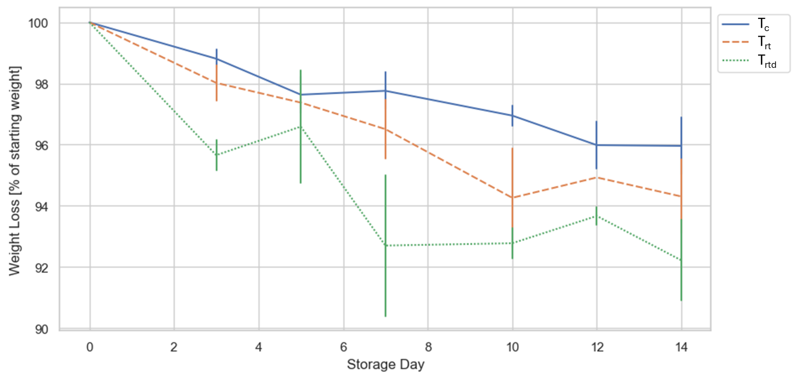
The data collected for the weight loss confirms the difference between the samples. Tomatoes stored at cooler temperatures show less weight loss than the tomatoes stored at room temperature (see: Figure 3). Požrl et al. [21] and Sualeh et al. [22] obtained similar results regarding the effect of temperature and weight loss. Javanmardi and Kubota [23] and Požrl et al. [21] attribute the weight loss to increased transpiration. Compared to refrigerated samples, tomatoes stored at ambient temperatures showed a greater weight loss over the storage period. Therefore, lower temperatures can help to prevent weight loss of fresh fruit [22]. However, storing fresh fruit at too low temperatures can cause chilling injury, which damages the tissues and leads to softening and rot [24,25].

In addition to temperature effects, physical damage also plays a critical role. Mechanically damaged tomatoes (T_rtd) exhibited even greater weight loss over the storage period. This trend can be explained by mechanical damage compromising the tomato’s natural protective barrier, leading to increased surface permeability and accelerated transpiration.

4.2.2. Color

Consumers often use tomato color as a quality indicator. Table 2 shows differences in the color development in the storage scenarios. These results suggest that tomatoes stored at lower temperatures (T_c) depict only minor differences in color change due to slowed-down ripening processes. In contrast, tomatoes stored in the T_rt scenario exhibited more pronounced and variable color changes, indicating a less controlled ripening process. The T_rtd samples followed a similar trend to T_rt, showing accelerated color degradation due to the combined effects of temperature and damage. The changes observed in the T_rt and T_rtd scenarios are consistent with findings from Sualeh et al. [22], who reported that tomatoes stored at ambient temperatures depicted faster visual changes than refrigerated samples. Additionally, Javanmardi and Kubota [23] demonstrated that elevated temperatures significantly influence lycopene development, further explaining the accelerated red color formation and variability in T_rt and T_rtd samples. However, the results obtained in this study exhibit a non-linear pattern, which may be attributed to the random sampling approach. Moreover, the color extraction method demonstrated limitations, as unintended elements, such as parts of the panicle and the metal positioning ring, were captured in the image mask (see Section 3.3). While individual CIELAB components provide insight into color changes, Požrl et al. [21] used the total color difference ($\Delta$E) as a more comprehensive metric for evaluating color shifts over time. Incorporating $\Delta$E into future analyses could offer a more sensitive and consumer-relevant assessment of color degradation during storage. Furthermore, we aim to explore alternative methods for color measurement, such as the use of a colorimeter, and compare these results to those obtained from image-based color recognition using RGB-images to create a more robust and standardized approach for assessing color as a quality parameter.

4.2.3. Aroma

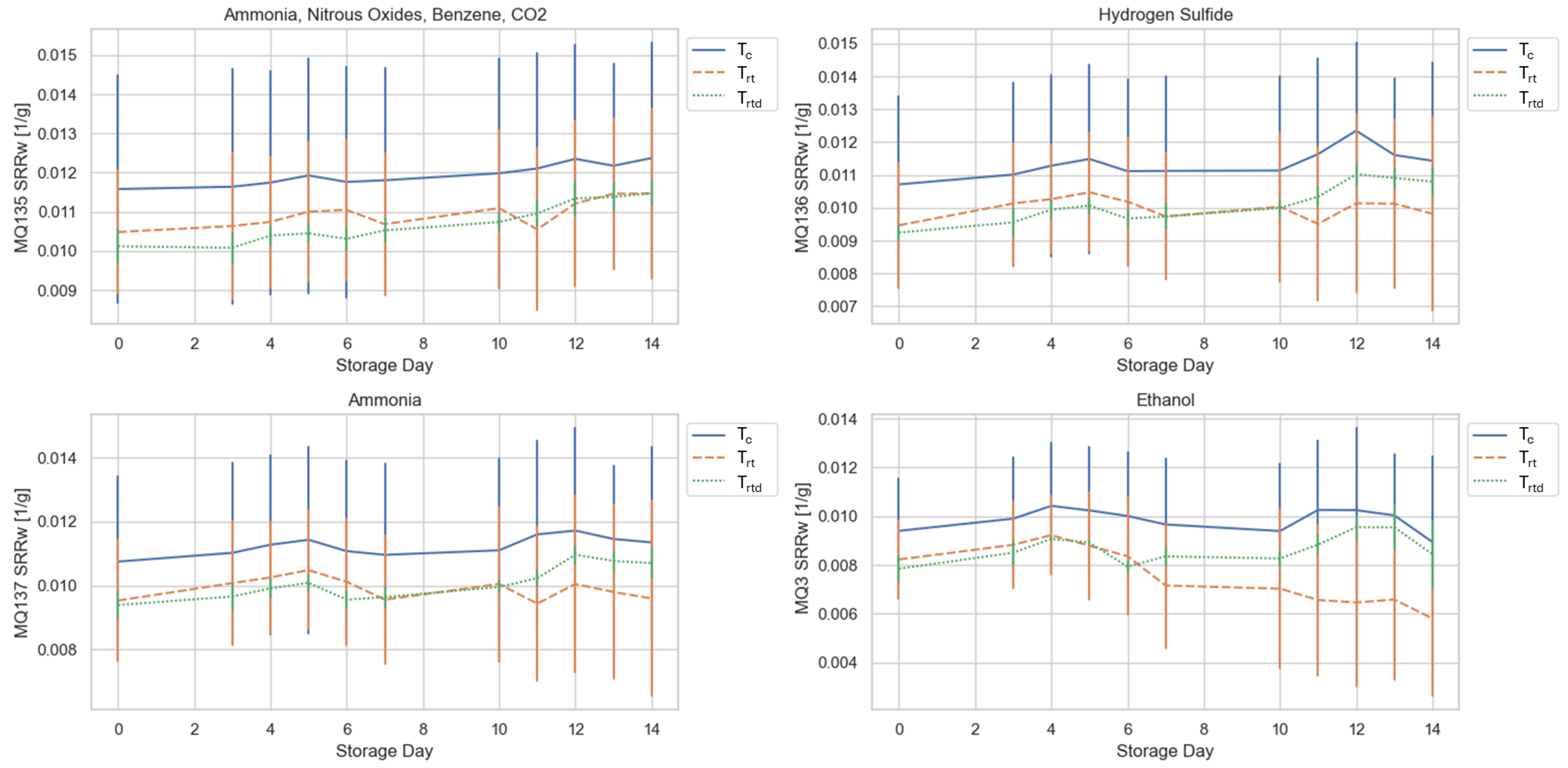
Aroma development in tomatoes is closely linked to post-harvest physiological and biochemical processes, which can be accelerated by mechanical damage [26]. In this study, E-Nose measurements captured the volatile profile of tomatoes across the storage period. As shown in Figure 4, the continuously monitored samples stored under T_c conditions exhibited similar sensor response patterns across the different sensors, suggesting a more stable and gradual development and degradation of aroma-related volatiles. Tomatoes stored at T_rt and T_rtd also depicted comparable sensor patterns, indicating similar shelf-life progress. However, at the end of the storage period, the T_rt samples showed a stronger deviation in sensor response than the T_rtd samples. The observed differences could indicate the presence of internal bruising, potentially caused by improper handling at an earlier stage in the food supply chain. Such damage is often not visible externally but can impact the aroma profile, leading to a decline in flavor quality [26]. Microbial infections could also contribute to an aroma profile change by producing spoilage-related volatiles. This is supported by the fact that one of the continuously monitored T_rt tomatoes showed signs of microbial spoilage at the end of the trial. Sinesio et al. [27] investigated the change in tomato aroma using E-Nose technology. They categorized samples into four classes based on visible defects and spoilage levels. Their results show that the E-Nose depicted a lower variance in classifying the samples than a trained sensory panel, highlighting this tool’s advantage. Hence, their study supports the finding that aroma profile alterations caused by damage or microbial spoilage can be detected and classified using E-Nose technology. Defining classes based on visible defects and spoilage levels could enhance new sample categorization and will therefore be investigated in future studies.

The influence of temperature on aroma development is also well-documented in the literature. Wang et al. [28] observed that low temperatures inhibited the production of aroma volatiles and an overall decrease in volatiles with extended storage time employing gas chromatography-mass spectrometry and E-Nose technology. Using the E-Nose data, they classified the tomato’s freshness into three categories. Similarly, Maul et al. [29] reported that tomatoes stored at lower temperatures tended to develop less aroma. They successfully classified the tomatoes, using E-Nose data, according to their freshness and storage temperature. In addition, they used gas chromatography to identify the responsible aroma components, linking them to the recorded E-Nose profiles. These findings aligned with the assessment conducted by a trained sensory panel, confirming that E-Nose technology can reliably detect temperature-related changes in aroma profiles. In general, the reduced production of volatiles also reflects a slower degradation process, potentially preserving freshness markers longer than high-temperature storage, which on the contrary can accelerate decay. Although our study revealed similar trends, it employed a new approach by using a weight-normalized sensor signal (SRR_w). To validate its applicability, our approach will be compared to already established methods in future studies. By incorporating a scale into the sample chamber, we can further streamline the process and thereby automate the weight measurement.

The combined analysis of color, weight loss, and aroma profiles on shelf life highlights that these parameters can help identify different storage scenarios and damaged samples. Therefore, they reflect key changes during post-purchase storage and indicate fruit freshness, making them informative features for machine learning models.

4.3. Machine Learning Pipeline

The steps of dimensionality reduction, training, and validation of the machine learning models are discussed below.

4.3.1. Dimensionality Reduction

Dimensionality reduction is a widely used technology for transforming high-dimensional data into a lower-dimensional space, improving processing speed for large datasets. Furthermore, the low-dimensional dataset can be used to visualize data in a more simplified way [30]. This study applied two classical linear transformation methods to the data: PCA and LDA. PCA is a frequently used dimensionality reduction method in E-Nose studies [10,27,28,31,32]. The quality of separation obtained in tomato samples differs between studies [10,27,28,31,32]. Hong et al. [32] successfully used PCA to separate tomato juice samples after different storage times. The separation of tomato grades based on E-Nose data and PCA was also observed [27,28]. Except for Sinesio et al. [27], all of these studies used the commercial E-Nose systems Airsense Pen2 / Pen3 (Schwerin, Germany). The Airsense systems use 10 MOS [33,34], which cover a range of target molecules similar to the E-Nose used in this study. Sinesio et al. [27], who employed an experimental E-Nose, achieved only partial separation of the samples. In the presented study, the level of random variation in the data was high, with sources traced to external influences and parts of the measurement procedure. Hence, PCA did not clearly separate storage days and storage scenarios, leading to its exclusion as a pre-processing step. Addressing these sources of variability should limit variation to the true differences within the sample, potentially making PCA a valid data dimensionality reduction method again. Therefore, future improvements in the measurement accuracy of the developed E-Nose system are expected to allow the PCA to be included as a potential pre-processing method in accordance with the aforementioned studies.

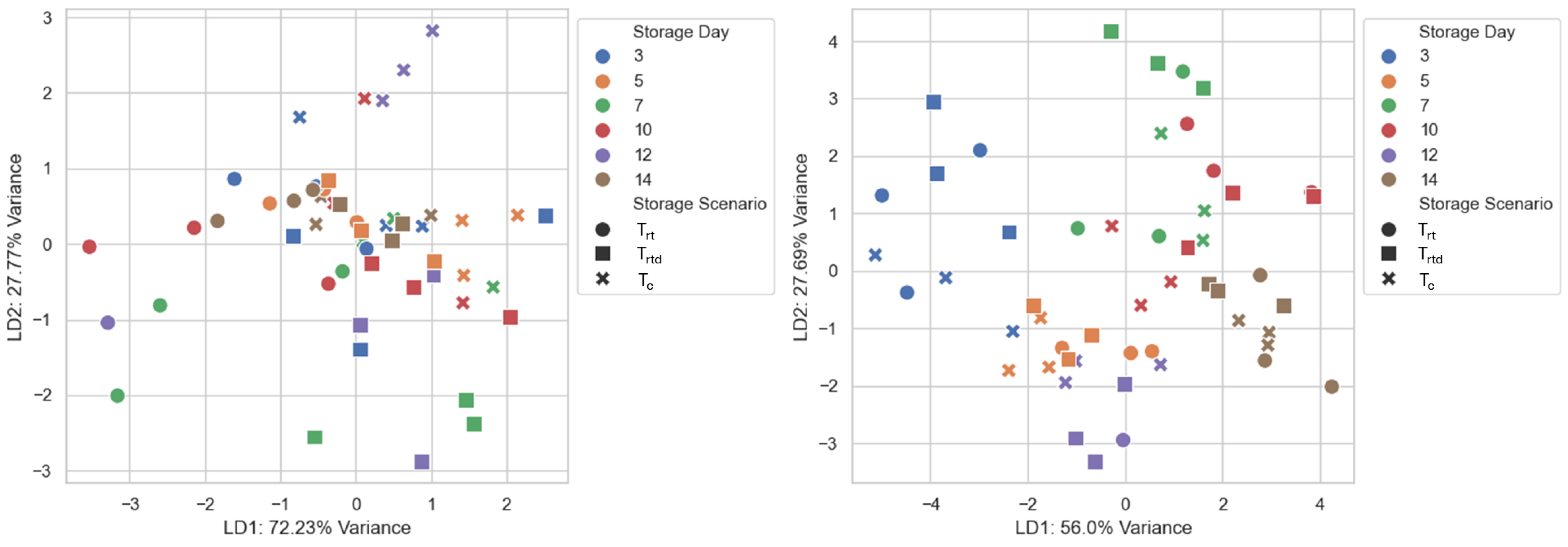
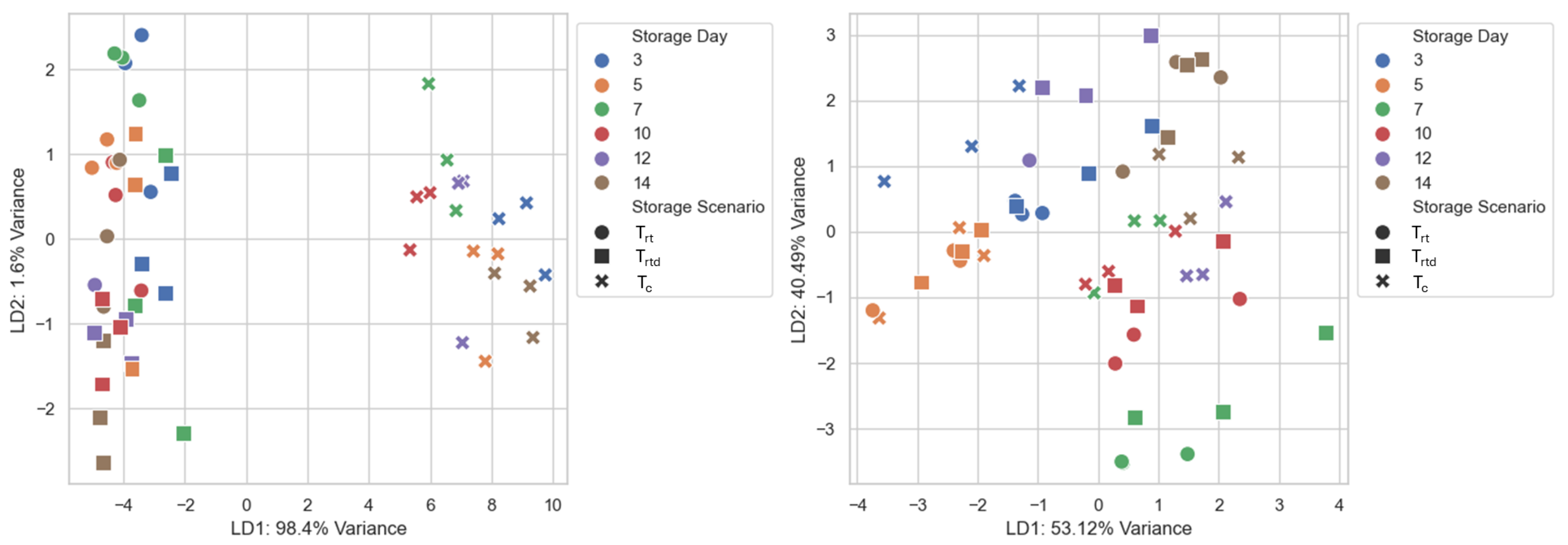
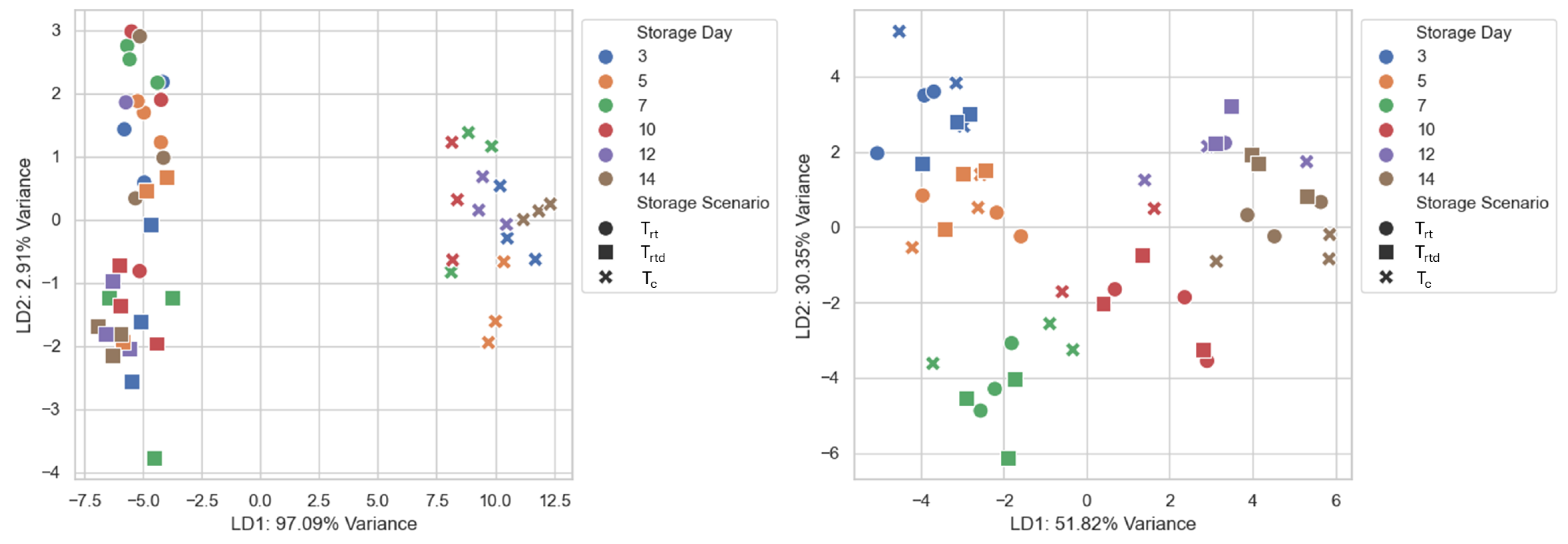
In contrast to PCA, LDA is a supervised data transformation, allowing the captured variation between classes and reducing the impact of uncertainties [35]. The LDA plots showed a clear separation of the data (see: Figure 5, Figure 6 and Figure 7). By including the SWC data, the separation could be greatly improved. Several studies have demonstrated the effectiveness of LDA in distinguishing freshness or quality-related stages in perishable food products using E-Nose data [10,12,17,31]. Sanaeifar et al. [12] applied LDA to monitor banana ripening by successfully separating different ripening stages and the onset of senescence. Similarly, Gómez et al. [31] perfectly separated four tomato ripening stages using LDA. In a subsequent study, they successfully separated storage days of tomato samples stored for twelve days and measured at three-day intervals [10]. Additionally, their studies concluded that LDA outperforms PCA in separating ripening stages [31] and measurement days [10]. Tang et al. [17] employed LDA to distinguish between freshness levels in coffee beans. Notably, they used the LDA results as input features for subsequent machine learning algorithms [17], similar to the presented study.

4.3.2. Classification Model Performance

The best model to classify storage days and storage scenarios was achieved using the combined dataset as feature input and applying LDA as a pre-processing step. This pipeline with SVC as the classifier achieved an accuracy of 72.91% for classifying the storage days and 86.73% for the storage scenario. Using kNN as classifier yielded a similar result for the classification of the storage scenario (see Table 3). In the literature, the most common variable classified based on E-Nose data is the ripeness of the fruit. Depending on the fruit and technology used, accuracy values between 72% (apple [18]) and 100% (banana [9]) were achieved. For example, Chen et al. [9] used a hybrid system of color detection and E-Nose. Using only the E-Nose, they were able to classify ripeness with an accuracy of 86–89%, depending on the machine learning model used. The algorithms based on only color recognition achieved 94–99% accuracy. By combining both technologies, most of their tested machine learning algorithms achieved an accuracy of 100% [9]. Huang et al. [36] developed a ripeness classification based on E-Nose and computer vision for tomatoes. The E-Nose system alone achieved an accuracy of 75%, the computer vision model had an accuracy of 85%, and the combination had an accuracy of 94%. Hong et al. [32] classified the storage days of freshly squeezed tomato juice. They achieved 86–97% accuracy for the E-Nose-based models and 96–98% in combination with an E-Tongue. Our best classification models for the storage days and storage scenarios achieved a performance range comparable to existing machine learning models applied to other classification tasks. However, the models based only on SRR_w data showed lower performance than those in other studies.

As previously mentioned, ripeness is one of the most used variable to classify fruits, which simplifies the classification task but may not reflect the complexity of post-purchase degradation of fresh produce. For consumers, the period between ripe and unfit for consumption is especially relevant, as most of the fresh produce is sold in a ripe state. Therefore, models to classify storage scenarios were trained without considering the specific storage days, while models to classify storage days were trained without distinguishing between the underlying storage scenarios. This approach was chosen to reflect realistic post-purchase conditions where either the storage duration or the prior handling of the product was unknown. This intentional introduction of additional variability evaluated whether the model could produce meaningful predictions despite the unknown pre-purchase histories of the tomatoes. However, this approach made the classification a more challenging task.

The performance achieved by the models in this study represents a good initial approach. In future studies, separating the storage scenarios during model training or incorporating storage-specific features could help reduce variability and improve classification performance. While some grouping was achieved (see Figure 7), the findings highlight the need for more consumer-relevant classification categories. Introducing predefined classes based on purchase conditions (e.g., ripeness, mechanical damage, microbial load) could improve model generalizability by enabling more accurate sample grouping rather than assuming uniformity based solely on visible indicators at the time of purchase. These groupings could be supported by microbial analyses to establish clearer links between sensor patterns and remaining shelf life. However, defining meaningful classes for products with unknown histories is challenging, as it requires the definition of reliable parameters to group them accurately.

In general, the proposed approach’s generalizability should be validated with a new dataset from comparable perishable fruits and vegetables (e.g., strawberries, blueberries, and bell peppers). Another approach could be to expand the current dataset with different tomato varieties, further supporting the model’s adaptability across a broader range of product characteristics.

4.3.3. Regression Model Performance

In addition to the classification models, regression models for the storage days were created. As with the classification models, two pre-processing methods and two machine learning algorithms (kNN regression and SVR) were compared. Predicting the storage day using the combined dataset and LDA as a pre-processing step showed promising results for both machine learning algorithms. The SVR model reached an MAE of 1.087 days, which shows an average deviation of about one day from the true storage day. The MSE of 1.707 and an R² of 0.865 indicate a good fit for the models, with a large portion of the variance being explained. For the kNN model, a lower MAE of 0.841 days was achieved with an MSE of 1.458 and R² of 0.867 yielding the best result for the regression task.

For comparison, Hong et al. [37] achieved a coefficient of determination R² of 0.974 for classifying storage days of freshly pressed tomato juice with a commercial E-Nose (Airsense Pen2, Schwerin, Germany) using PCA and partial least squares regression. Their root mean squared error (RMSE) of 0.830 was lower than the errors observed in this study.

Despite the good overall performance, the results show that predicting the exact storage day remains challenging. However, considering tomatoes’ relatively long shelf life, the level of variance observed in the predictions is acceptable. Nevertheless, predictive accuracy is expected to improve with further system adjustments, such as reducing external variability by implementing filtered air and enhancing measurement precision.

4.4. Threats to Validity

While this study’s results provide promising insights into the potential of combining sensor-based measurements and laboratory data with machine learning to assess tomato shelf life, several limitations that may affect the validity of the findings must be acknowledged.

The study was based on a single 14-day measurement run. Measurement days included the data collection of multiple tomatoes per day and storage scenario. Although this approach provided several data points across the storage period, conducting the experiment only once limits the model’s generalizability. Additionally, the dataset used in this study was relatively small. Therefore, further trials with larger sample sets must be conducted to build a more robust and generalizable model.

Although the samples were visually inspected upon purchase, some may have experienced improper handling at earlier stages in the food supply chain. Internal bruising, stress, or a different state of ripeness, which were not visually detectable, could have introduced variability. Another potential source of variability could be improperly maintained storage conditions in earlier stages of the supply chain. In future studies, introducing predefined classes based on ripeness or pre-purchase conditions (e.g., mechanical damage, microbial load) could improve the model’s generalizability by allowing purchased tomatoes to be assigned to the appropriate class rather than assuming uniformity on the day of purchase. Nevertheless, this highlights the challenge of examining pre-purchase conditions for consumers in real-world scenarios and the need for further research.

Several constraints may have influenced the data quality of the E-Nose system. Unfiltered air, potentially containing other VOCs, was used to clean the system. These VOCs might have affected the sensors’ baseline resistance, leading to measurement deviations. Additionally, the high pump flow rate may have led to an uneven distribution of the VOC concentration inside the E-Nose. The sensors were not calibrated due to their broad sensitivity and low specificity, which can lead to increased measurement variability across samples. However, the focus of this study was to monitor relative changes within the product over time rather than quantifying specific compound concentrations. Moreover, the limited resolution of the analog-to-digital converter may have affected the data quality, potentially reducing the precision of the recorded sensor signals. An additional challenge is long-term sensor drift, which can further contribute to measurement variability.

The established system and machine learning pipeline showed strong potential as a foundation for further research. Future work should refine the measurement system, increase sample size, and repeat trials under varying conditions to enhance the reliability and applicability of the proposed approach. Furthermore, alternative strategies for deriving representative values from the continuous E-Nose signal to identify the most suitable input for robust model development should be investigated. Additionally, it would be possible to measure and integrate the influence of packaging, especially of new bio-based materials [38]. Despite these limitations, the study successfully demonstrates the feasibility of using color, weight loss, and volatile profiles as shelf-life-related parameters for distinguishing storage days and storage scenarios.

5. Conclusions

Monitoring the freshness and spoilage of food is essential to ensure consumer safety and to minimize avoidable food waste. However, traditional methods for assessing fruit quality are often destructive, time-consuming, and expensive. This study demonstrates that storage scenarios and storage days can be predicted using a data fusion approach, including storage data, weight loss tracking, color data, and volatile profiles recorded by the developed E-Nose system.

Tomatoes purchased from the supermarket exhibited high variability, limiting the interpretability of the data. While trends of the SRR_w data were observed for the continuously monitored tomatoes, the differences became less pronounced under random sampling conditions. The randomly sampled SRR_w data was used for the machine learning models. Including the SWC data improved the separation and modeling of the storage days and storage scenarios. The best results were obtained when LDA was applied as a pre-processing step with the combined dataset. The highest classification performance was achieved using SVC with LDA and the combined dataset, reaching 72.91% accuracy for the storage day classification and 86.73% for the storage scenario. For the storage scenario, the kNN classification showed similar performance metrics (accuracy: 86.73%).

Among the regression models, the kNN performed best when trained with the combined dataset with LDA as a pre-processing step, achieving an R² of 86.69%, an MAE of 0.841 days, and an MSE of 1.458. The SVR model produced an MAE of 1.087 with an MSE of 1.707 and an R² of 86.54% showing a slightly worse performance compared to the kNN.

While the E-Nose system demonstrated its potential for capturing differences in tomato quality parameters, several limitations currently hinder its generalizability. Sensitivity to environmental conditions—such as temperature, humidity, and VOC contamination in the fresh air-as well as procedural factors like high pump flow rates and limited data resolution affected the consistency of the measurements. Moreover, the generalizability of the results is further limited by the fact that only a single measurement run was conducted, with multiple recordings taken over a 14-day storage period.

Future work should focus on refining the system by incorporating filtered and dried air, optimizing flow rates, and enhancing signal resolution. With these improvements and including a broader and more diverse dataset, the system’s accuracy and robustness are expected to improve, enabling more reliable and generalizable conclusions. Since assigning classes to products with unknown histories remains challenging, future research will prioritize predictive approaches that estimate remaining shelf life rather than categorical classification. These can be important steps towards a vision of digital food twins [39,40].