The Use of Low-Cost Gas Sensors for Air Quality Monitoring with Smartphone Technology: A Preliminary Study

Abstract

In the past decades, both low-cost gas sensors for air quality monitoring and smartphone devices have experienced a remarkable spread in the worldwide market. Smartphone devices have become a unique tool in everyday life, whilst the use of low-cost gas sensors in air quality monitors has allowed for a better understanding of the personal exposure to air pollutants. The traditional technologies for measuring air pollutant concentrations, even though they provide accurate data, cannot assure the necessary spatio-temporal resolution for assessing personal exposure to the various air pollutants. In this respect, one of the most promising solutions appears to be the use of smartphones together with the low-cost miniaturized gas sensors, because it allows for the monitoring of the air quality characterizing the different environments frequented in everyday life by leveraging the capability to perform mobile measurements. In this research, a handheld air quality monitor based on low-cost gas sensors capable of connecting to smartphone devices via Bluetooth link has been designed and implemented to explore the different ways of its use for assessing the personal exposure to air pollutants. For this purpose, two experiments were carried out: the first one was indoor monitoring of CO and NO₂ concentrations performed in an apartment occupied by four individuals and the second one was mobile monitoring of CO and NO₂ performed in a car cabin. During the indoor measurements, the maximum value for the CO concentrations was equal to 12.3 ppm, whilst the maximum value for NO₂ concentrations was equal to 64 ppb. As concerns the mobile measurements, the maximum concentration of CO was equal to 8.3 ppm, whilst the maximum concentration of NO₂ was equal to 38 ppb. This preliminary study has shown that this system can be potentially used in all those situations where the use of traditional chemical analyzers for measuring gas concentrations in everyday life environments is hardly feasible, but also has highlighted some limits concerning the performance of such systems.

1. Introduction

According to the WHO [1], air pollution is one of the biggest concerns for human health seeing as over 90% of people live in regions where the safe limits are systematically exceeded. Poor air quality affects both outdoor and indoor environments, as proven by several institutions [1,2,3,4]. For this reason, air quality monitoring is of the utmost importance because it can provide a tool for governments and regulatory bodies to effectively assess the levels of pollution to which the population is exposed.

The instruments traditionally used by the dedicated institutions to measure air pollutant concentrations are bulky, expensive, and requires relevant infrastructure and resources for their operation [5,6,7,8]. As a consequence, in most cases, few monitoring fixed stations are available on a territory, and therefore, it is hardly feasible to gather air pollutant concentration maps with a good spatio-temporal resolution. Moreover, it can happen that no monitoring station is available to cover whole regions, as is the case in many emerging countries [9].

To address this issue, remarkable attention has been given recently to low-cost miniaturized gas sensors (LCSs) and monitors (LCMs) based on their functioning [10,11,12]. Some of them have achieved a significant level of maturity and are already available on the worldwide market (e.g., resistive sensors, electrochemical cells, non-dispersive infrared radiation absorption sensors, and photo-ionization sensors) [13,14,15], whilst, in other cases, their development can be considered still in a preliminary study phase [16,17]. In both cases, such devices are considered an appealing option due to their high grade of miniaturization level, affordability, low power consumption, and ease of use [18,19].

Despite all these positive aspects, the use of LCSs and LCMs in air quality monitoring is still a matter of investigation for research groups due to some limitations affecting the technology that make them less accurate when compared to the traditional instruments [20,21,22]. The performance of LCSs, and consequently, of LCMs, is influenced by both meteorological and environmental conditions [23,24,25], and also by the type of technology implementing them. In particular, the presence of interfering gases [26,27,28], the temperature, and ambient humidity changes can represent a disturbing factor which affects the LCS measurements to different degrees [29,30,31], depending not only on the type of sensor, but also considering different copies of the same sensor manufactured in the same batch. To mitigate the adverse influence of these variables, the scientific community has explored various countermeasures, mostly consisting of the elaboration of sensor output signals performed by suitable software through which various algorithms are implemented, aiming at correcting the LCS or LCM measurements [32,33,34].

Even though it is commonly recognized that the performance of LCMs cannot still be compared with the traditional and professional instruments usually used by governmental agencies [35], it appears clear that in some circumstances they are the only viable way to carry out air pollutant concentration measurements in real time. As a matter of fact, households or common citizens cannot afford bulky and expensive instruments to monitor their homes or apartments, or even to assess their personal exposure to air pollutants during their everyday life in vehicle cabins, public buildings, or on public transport. If we recognize that air pollutant concentrations can significantly vary in urban microenvironments or streets very close each other [36], or that indoor air quality can be remarkably worse than the outdoor one [37] in some cases, it also clearly appears that personal exposure assessment to air pollutants cannot be accomplished by sparse, fixed monitoring stations. Therefore, the use of LCMs appears to be the only way to obtain indications about personal exposure to air contaminants, especially if we consider that the most effective way to accomplish this task is to perform mobile measurements.

To carry out such measurements, it is preferable that the tool or device to use has specific features, such as handheld sizes, battery-power operated, capability to operate both in indoor and in outdoor environments, and capability to track or store the measures. LCMs already available on the market do not always present all these characteristics; moreover, most of times, the manufacturers of such devices do not provide information about their accuracy or data about their calibration, therefore, the reliability of their measurements can be questionable.

This preliminary study is aimed at exploring the capabilities of a handheld monitor based on electrochemical gas sensors and designed to operate together with a smartphone device. Using a smartphone in conjunction with handheld monitors provides more flexibility for air quality monitoring in all the situations in which research-grade and accurate instruments, such as gas chemical analyzers, cannot be deployed or are hard to arrange and use due to their bulkiness. For example, more handheld monitors can be used to set up an indoor air quality monitoring network composed of several nodes, each of them represented by a handheld monitor deployed in a room, whilst a smartphone can act as a hub which collects the measurements of the various nodes through Bluetooth connections. Combining the use of such monitors with smartphones enables a very easy and quick way to set up local monitoring networks for the air quality monitoring of indoor environments composed of multiple rooms or spaces without using third services, such as, cloud services or wi-fi local networks. Considering that almost all citizens own a smartphone, this feature can provide immediate access to the air quality data of public spaces, such as, airports, hospitals, or public offices, for any user. The same structure can also be used for performing mobile measurements, such as the air quality monitoring in a car cabin during a trip.

In this preliminary study, two experiments were performed to test the capabilities of a handheld monitor, called “DSnasus”, designed and implemented in our laboratories to be used with a smartphone. In the first experiment, two monitoring units were deployed in two rooms of an apartment to form a little monitoring network with the smartphone, as earlier briefly explained, to measure carbon monoxide and nitrogen dioxide concentrations. In the second experiment, one of the two monitors was used in a car cabin during a trip to perform mobile measurements of carbon monoxide and nitrogen dioxide concentrations.

2. Materials and Methods

In this section, we are going to describe the structure and functions of the devices under evaluation, the methods used to calibrate the sensors, and the setting up of the two experiments.

2.1. The Devices and the Sensors Used for the Experiments

Two units of the designed handheld monitor were implemented for the experiments. Moreover, a smartphone, featuring an Android operating system, was used to complete the necessary hardware (see Figure 1).

On each of the two monitoring units, two electrochemical gas sensor types were mounted. The first one was the CO-B4 by Alphasense, dedicated to CO concentration measurements, and the second one was the NO2-B43F, dedicated to NO₂ concentration measurements. These sensors are designed for measuring ambient concentrations of gas, as stated by the manufacturer. In

Table 1. Main technical specifications of CO-B4 and NO2-B43F sensors.

Sensor	Sensitivity	Response Time	Zero Current	Range
CO-B4	+420/+650 nA/ppm	<30 s	+30/−250 nA	1000 ppm
NO2-B43F	−200/−650 nA/ppm	<80 s	−80/+80 nA	20 ppm

, a summary of their technical specifications provided by Alphasense is reported to give an idea of their capabilities.

Both sensors are enclosed in identical cases and are the same size. They are amperometric sensors featuring four electrodes, as can be seen in Figure 2. Their working principle is exposed in the Baron and Saffell article [38]. Basically, they have four electrodes; the counter and the reference ones are necessary for the correct operation of the sensors, whilst the auxiliary and the working electrodes provide the sensor outputs, represented by weak electric currents. The counter, reference, and working electrodes are separated by the wetting filters. On the working electrode the reduction or oxidation of the gas molecules takes place (depending on the gas species). It is coated with a catalyst to facilitate the reaction with them. This reaction generates electronic charges which are balanced by a second reaction at the counter electrode, forming with the first one a redox pair of chemical reactions. When the sensor is exposed to clean air, the counter electrode is at the same potential as the working one, while in the presence of the target gas their potential changes. In this way, a potential difference between the working and counter electrodes is generated, and consequently, an electric current at the working electrode starts to flow, providing the output of the sensor. The auxiliary electrode is not exposed to the target gas, but it reflects the fluctuations of the sensor baseline. The electrochemical sensors are sensitive to the temperature and humidity changes, which affect both the sensor sensitivity and their zero current. Another challenge posed by the use of electrochemical sensors is the so-called cross-sensitivity effect. As a matter of fact, sensors designed for measuring a specific gas, for example, nitrogen dioxide, can be influenced by the presence of other gases (named interfering gases), which modify the correct measurement depending on their concentrations.

Despite the aforementioned adverse aspects, electrochemical sensors present some advantages if compared with other sensor types commonly used for pollutant gas monitoring, such as the chemiresistive sensors. They feature a lower power consumption and also a lower cross-sensitivity [39], and for these reasons they were selected to implement this monitor. As stated by the manufacturer, both the sensors can measure very low gas concentrations (less than 100 ppb) [40,41] if supported by an adequate electronic board. To achieve this goal, the electronic circuitry must be able to adequately amplify the weak electric currents representing the sensor output and limit the electronic noise affecting these signals at the same time. We designed and implemented an on-purpose electronic board for the sensor use, and its characteristics are exposed in detail in a previous article [42].

The sensors used in this experiment are equipped with a membrane which helps to filter out some interfering gases, limiting the cross-sensitivity effect for some gas types. The NO2-B43F sensor has a membrane made of MnO₂/PTFE microparticles which helps to filter out the main sensor interfering gas: ozone [28,40,43]. As concerns the CO-B4 sensor, the manufacturer reports in its datasheet that it is equipped with a filter for limiting the effects of one of the main interfering gases: hydrogen sulfide [41]. Other interfering gases are hydrogen for the CO-B4 and chlorine for the NO2-B4 [40,41]. In this respect, the effects of such gases are expected to be reasonably negligible due to their expected very low concentrations in the environments explored in this study.

As concerns the design of the handheld monitor, it is based on three modules implemented by three printed circuit boards: the sensor board [42], the data elaboration/interface board, and the Bluetooth module. The first two modules were designed in our laboratory, while the Bluetooth module is the RN42XV by Microchip. The electronics featuring the sensor board are able to read the weak electric currents representing the outputs of the sensors, opportunely amplify them, and convert them into voltage signals [42]. These constitute the inputs for the data elaboration/interface board, which digitalizes them. The voltage signals reflect the gas concentrations affecting the sensors; their digitalization and the subsequent elaboration is performed by the microprocessor PIC18F4652 by Microchip, which is the core of the module. The firmware running on the microprocessor is in charge of performing both the data elaboration function and the interface function. The data elaboration consists of clearing the input signals by removing or limiting the electronic noise affecting them through a numerical filter based on the rolling average smoothing technique. Subsequently, the mathematical law for converting the sensor signals into values expressing the gas concentrations is applied. The measures of the gas concentrations composing the outputs of the elaboration so far described can be transmitted via Bluetooth to a smartphone, acting as the master device. Optionally, they can also be transmitted via the USB port available on this module. In both cases, the connection between the handheld monitor and a smartphone device, or a PC connected via USB, follows the “master-slave” scheme; in this respect, at the sampling rate selected by the user, the smartphone requests the monitor for the current gas concentrations, which will transmit them using the Bluetooth or USB channel. The data elaboration/interface board also has the necessary electronic circuitry for managing powering the monitor. It is typically powered by its internal ion-lithium battery, which is recharged using the USB socket. A standard smartphone battery charger plugged into the USB socket can be used to recharge its battery, or optionally, the battery recharge will be active whenever the monitor is connected to a PC USB port.

As mentioned earlier, the connection of the DSnasus monitor with the smartphone or PC follows the master/slave architecture. Therefore, the specific App running on the smartphone (which is the device acting as master) sends to the monitor (which is the device acting as slave) the specific command at the sampling rate selected by the user to retrieve the current gas measures. These measures are shown to the user and written in a file stored on the local memory of the smartphone to form the dataset. Obviously, the file containing the measure records can be subsequently downloaded from the smartphone for further analysis. As concerns the selection of the sampling rate, it can be carried out by the smartphone user through the App earlier mentioned, designed also to perform all the necessary tasks, comprising the searching of DSnasus monitors operating in the vicinity and the Bluetooth connection management. This App, designed in our laboratory, was developed for Android operating systems. The main advantage provided by the use of smartphone devices with handheld monitors connected via Bluetooth consists of the possibility of easily setting up multiple star-shaped local networks, as depicted in Figure 3, without the need for a third support, such as, cloud services or similar. The maximum number of connections, and therefore of DSnasus monitors, that the system can manage is 255. The use of local networks composed of several monitors can be helpful for the air quality monitoring of indoor environments, such apartments or public offices, formed of several rooms or spaces which can be separated by doors or structures that create micro-environments not necessarily connected to each other. For this preliminary study, we prepared just two monitors to form a simple network for performing a preliminary test of the idea at the base of the system, as described in this document.

2.2. The Calibration of the Sensors

An important step of the experiment was the calibration of the sensors. It consisted of finding the mathematical law which allowed us to convert the voltage signals into gas concentrations. To perform this task, laboratory tests were performed by using a test chamber in which the two monitors were introduced. In this chamber, known gas concentrations were injected using a mass flow controller and the real gas concentration inside it was monitored by regulatory-grade instruments which acted as reference for the measurements.

By having the sensors a highly linear response, we decided to use the multivariate regression technique to convert the voltages into gas concentrations. Thus, the conversion law is as follows:

GC = aV_w + bV_A + c

(1)

where GC is the gas concentration expressed in ppm, in the case of CO measurements, or in ppb, in the case of NO₂ measurements; V_w and V_A are the voltage signal of the working and auxiliary electrode, respectively; and a, b, and c are the coefficient to find for calibrating the sensors. The method used to find the a, b, and c coefficients was the ordinary least square (OLS) algorithm, available in many software tools or libraries for scientific purposes. In this study, the software Origin 7.0 by Originlab was used for calculating the coefficients. The quality of the calibrations carried out by the laboratory tests was evaluated by using the coefficient of determination (R²) and the mean absolute error (MAE) computed by comparing the reference data with the ones produced by the calibration law of each sensor.

2.3. The Indoor Monitoring

For the indoor monitoring, two units of the DSnasus monitor were used in an apartment occupied by four individuals. This monitoring was carried out during their everyday activities. The first monitor was placed in the kitchen of the apartment, while the second monitor was deployed in the living room (see Figure 4 and Figure 5). In this way, it was possible to test a little local network composed of the two monitors. The two rooms were separated by a sliding door kept almost always open. The decision to deploy the monitors in this area of the apartment was taken because a previous study [28] has shown that this is the place where one is likely to measure gas emissions due to the presence of various sources, such as, methane gas burners, cigarette smoke, or candles. The monitors were fixed to the wall of the rooms, roughly two meters high. The living room had a door giving access to a balcony, same also for the kitchen. During the experiment, the two doors were partially opened for some minutes to ensure a minimum of air exchange, but avoiding significantly modifying the temperature and the humidity inside the apartment. The thermostat of the apartment heating system was kept at 20 °C to ensure steady thermal conditions as close as possible to the conditions registered during the calibration process. As concerns the humidity values, a dehumidifier placed in the living room was set to a relative humidity equal to 50% to reproduce the environmental conditions met during the calibration process. The unit placed in the kitchen had the sensors denoted as NO₂(1) and CO(1), while the unit placed in the living room had the sensors denoted as NO₂(2) and CO(2). The distance between the two units was 7.2 m.

Before deploying the units in the apartment, the firmware of the microprocessor inside the monitors was updated by inserting the conversion law with the values of the coefficients found after the calibration process. The possibility to update the conversion law or change its coefficients or parameters is an important aspect of this monitoring system. It is important to underline that monitors or systems based on low-cost gas sensors having the same feature are not always available on the worldwide market currently.

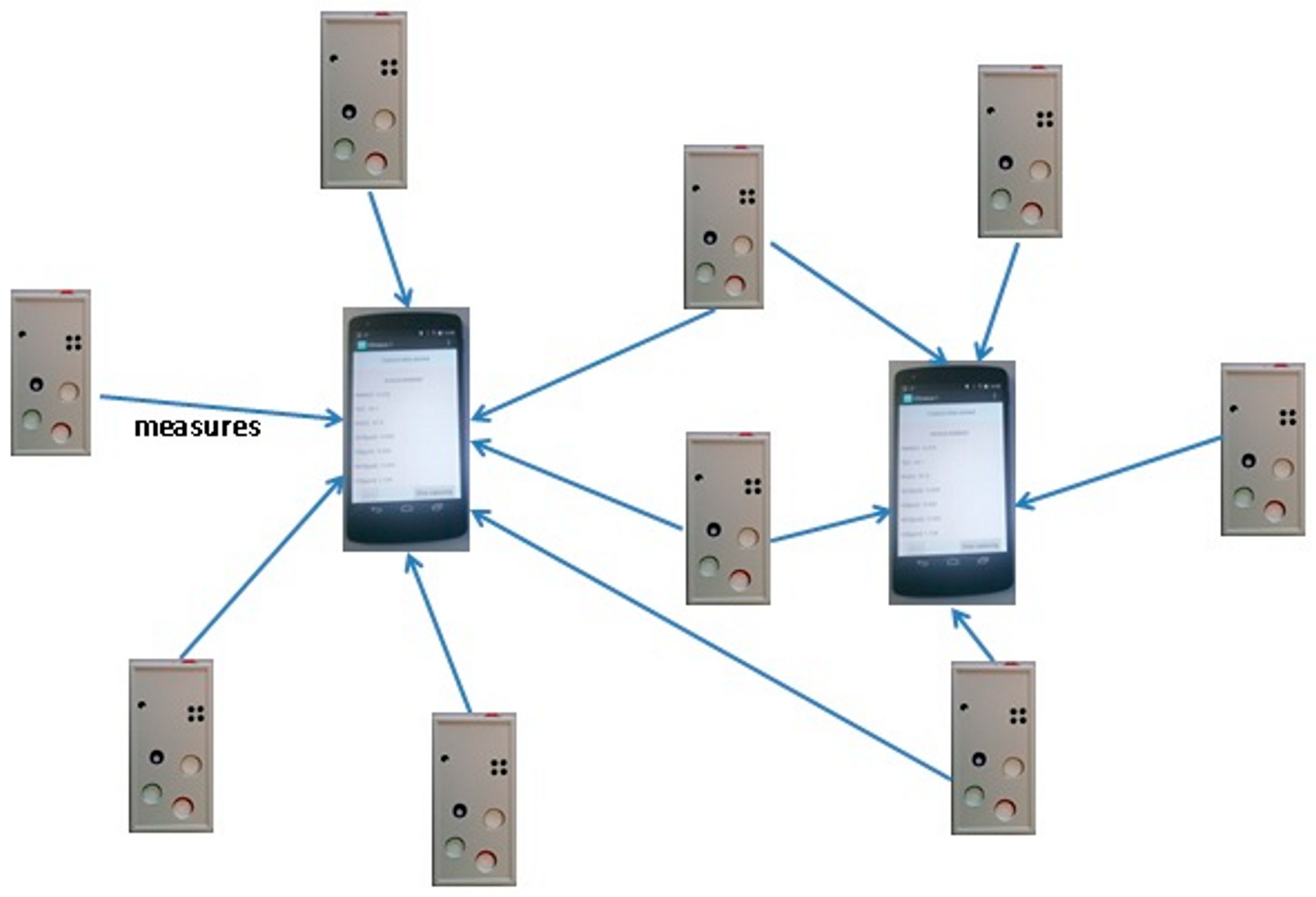
2.4. The Mobile Monitoring

The unit used for monitoring the concentration of CO and NO₂ in the car cabin was placed on the car dashboard using an ordinary smartphone holder available in any store selling car accessories (see Figure 6). The air conditioning system of the car was set to 20 °C, whilst the car windows were kept closed during the duration of the experiment and the forced ventilation was set to the minimum. These precautions were aimed at preserving the car microclimate as close as possible to the conditions characterizing the calibration operations. The route run by the car was formed of extra-urban and urban roads to ensure a certain amount of variability of environments and gas concentrations. For this preliminary study, we carried out the experiment by making a trip in a diesel fueled car on which the particulate filter was absent.

3. Results

The data concerning calibration of the sensors, along with the data related to the indoor and mobile measurements, are provided in the Supplementary Materials section. Hereinafter, the results related to the calibration, indoor, and mobile measurements are exposed in three distinct subsections for an easier reading.

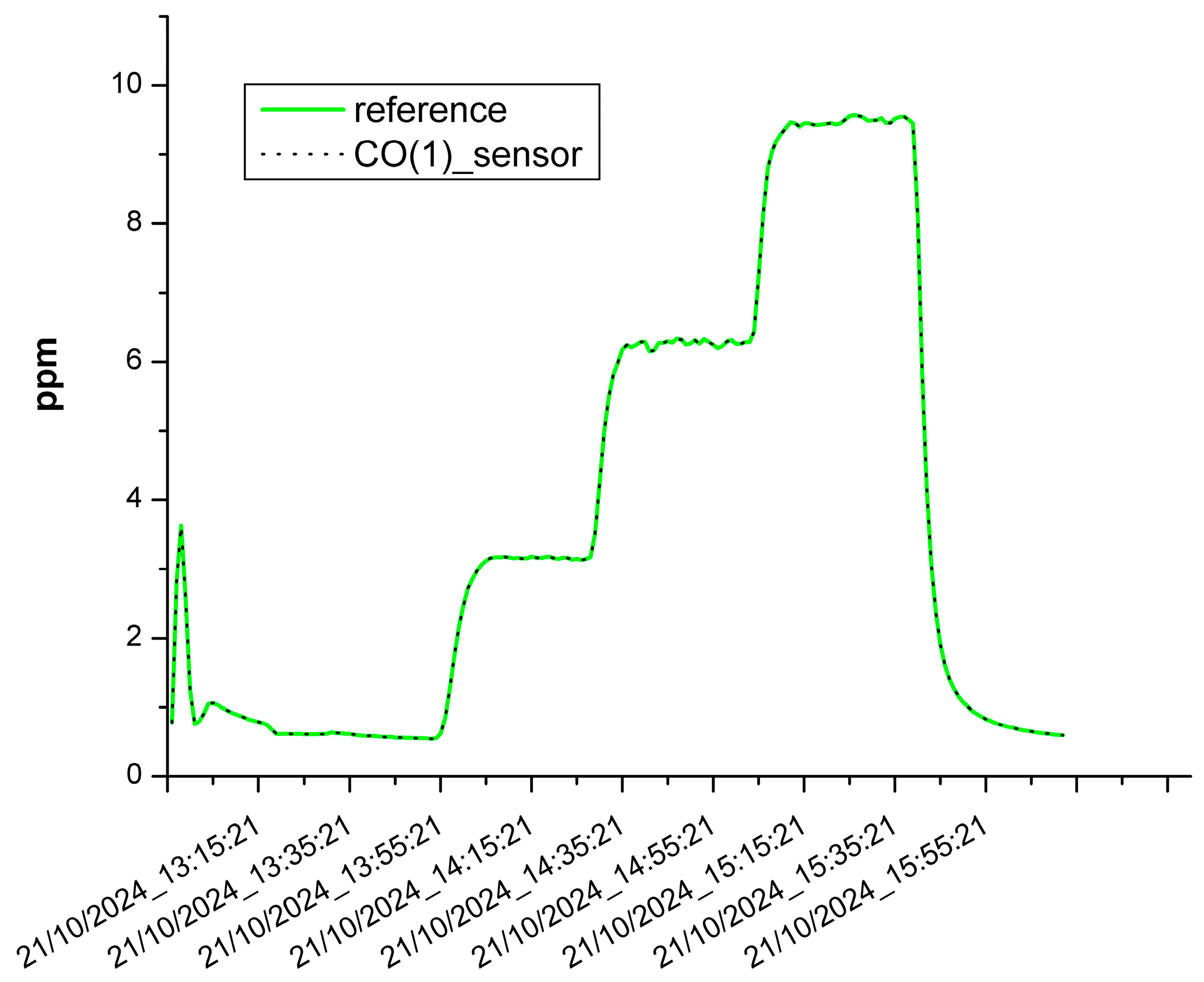
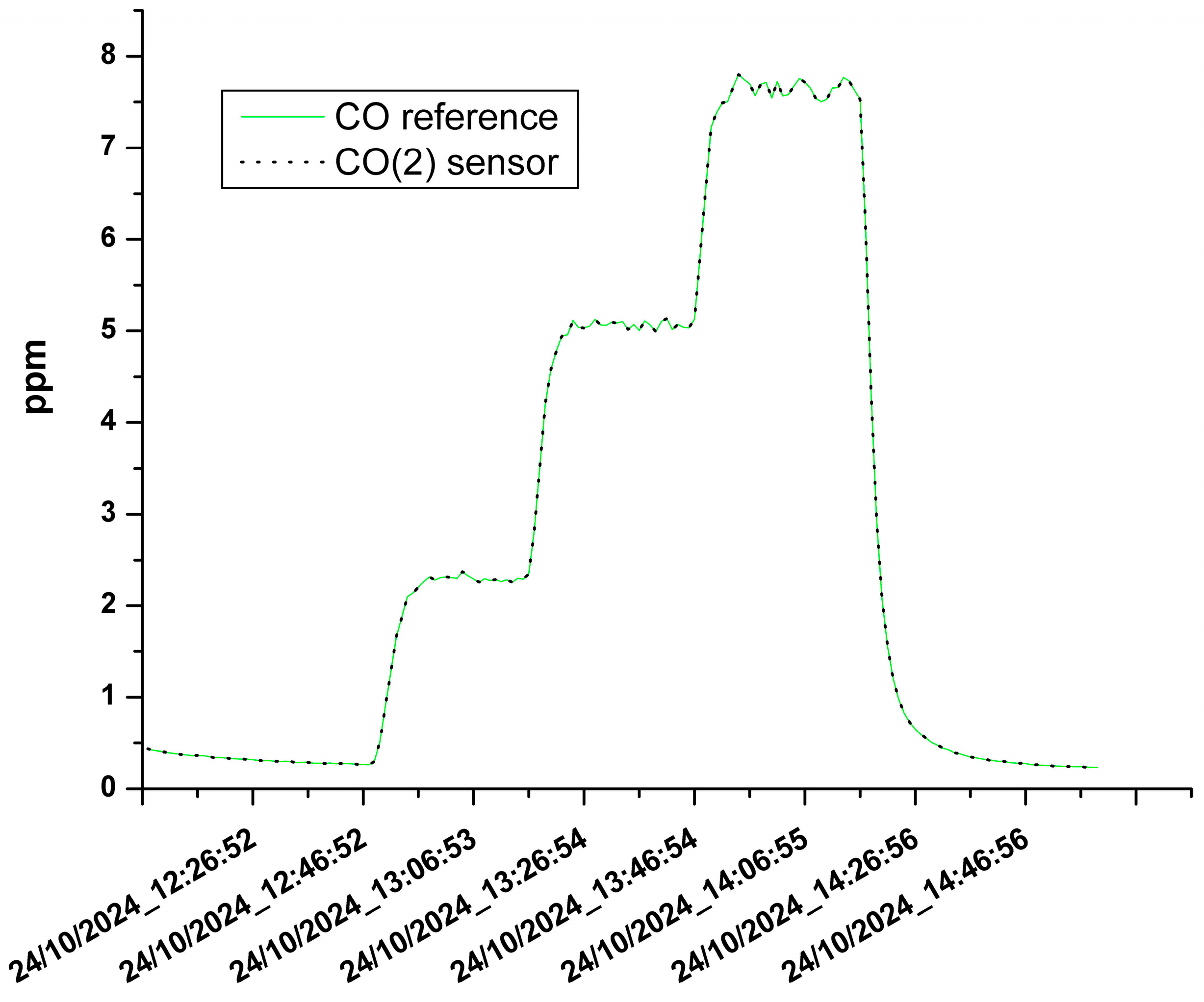
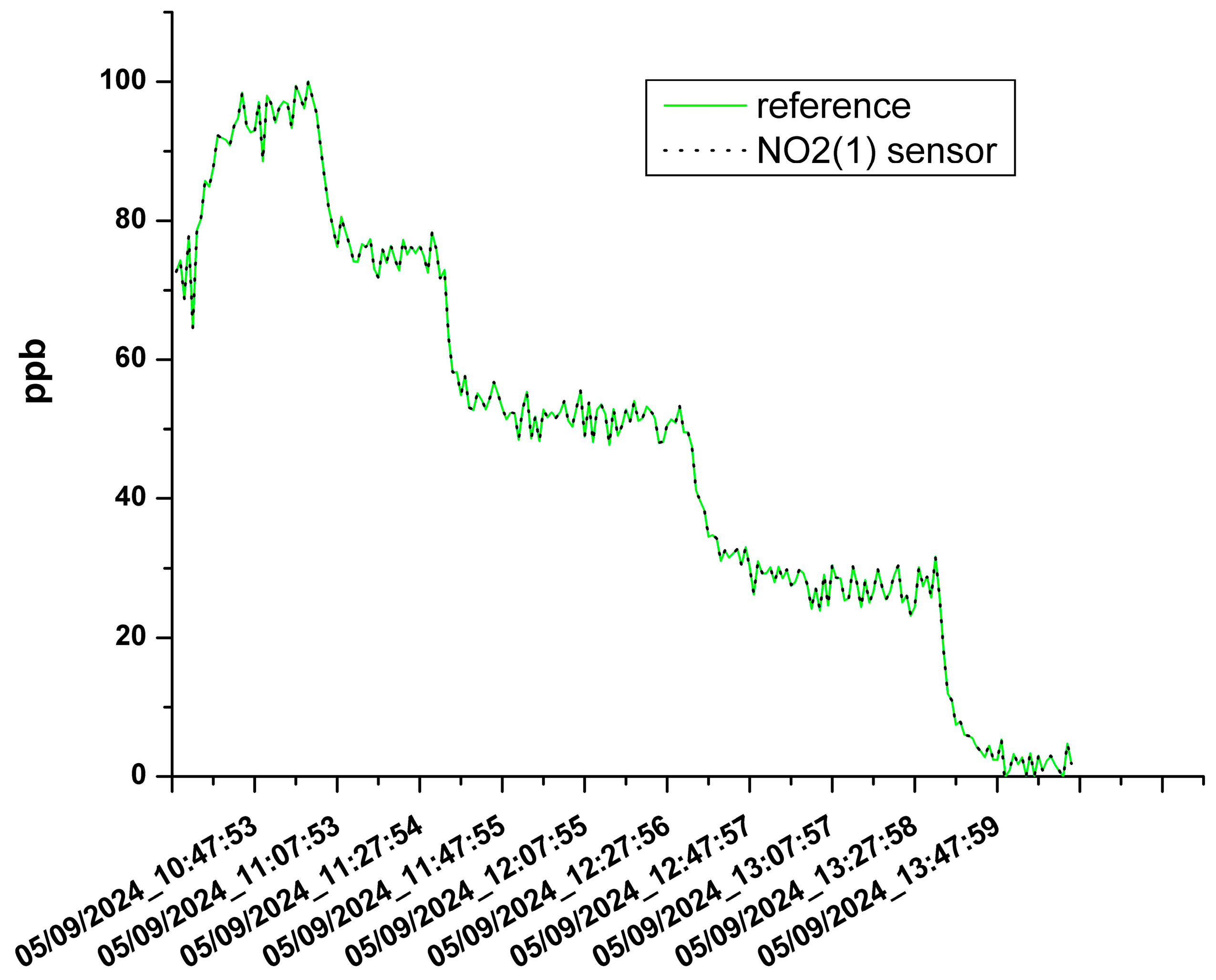
3.1. The Results of the Sensor Calibration

The calibration of the sensors was performed using a dataset formed of records containing both the sensor voltage output signals and the measures of the reference instrumentations. The sampling rate was set to one minute, whilst the concentration of CO and NO₂ injected into the test chamber were selected to cover the typical range measurable in the indoor or outdoor environments (see Figure 7, Figure 8, Figure 9 and Figure 10). The quality of the calibration can be evaluated by inspecting

Table 2. Coefficient of determination (R²) and MAE found for each sensor after calibration.

Sensor	R2	MAE
CO(1)	0.999	0.001 ppm
CO(2)	0.999	0.0009 ppm
NO2(1)	0.999	0.053 ppb
NO2(2)	0.995	1.415 ppb

, where the coefficient of determination and the MAE are exposed for each sensor. In

Table 3. Coefficients of the conversion law found for each sensor.

Sensor	a	b	c
CO(1)	−3150 ppm/V	3.127 ppm/V	6.243 ppm
CO(2)	−2.762 ppm/V	2.705 ppm/V	5.239 ppm
NO2(1)	104.933 ppb/V	−103.909 ppb/V	93.010 ppb
NO2(2)	98.294 ppb/V	−97.607 ppb/V	91.989 ppb

, we can see the values of the coefficients of the conversion law found for each sensor. The figures here are exposed and the values of R² greater than 0.9 found for each sensor show a good quality of the calibration. As a matter of fact, values of R² very near to 1 denote a good capacity of the monitors to follow the variations in the real gas concentrations. The good quality of the calibration, and therefore of the conversion law, is confirmed by the MAE value of each sensor as they are in the range of 0.001 ppm to 0.0009 ppm for the CO sensors, and 0.053 ppb to 1.415 ppb for the NO₂ sensors. As concerns the temperature and the relative humidity values, we observed very limited variations during the calibration of each sensor, as expected, ranging from 18.6 °C to 21.2 °C for the temperature and from 39.5% to 53.7% for the relative humidity. As can be found on the sensor manufacturer website, the variations registered for both these environmental parameters do not significantly affect the response of the sensors due to the fact that their range is limited enough.

3.2. The Results of the Indoor Monitoring

The indoor experiment started on the 23rd of November 2024 and finished on the 25th of November 2024. The sampling rate of both the monitors was set to one minute, producing a dataset composed of 2930 records. The temperature and the relative humidity did not vary significantly during the experiment, ranging from 16.7 °C to 21.2 °C, and from 38.8% to 54.2% for the humidity. Moreover, the mean and median values for the temperature were, respectively, equal to 19.5 °C and 19.9 °C, while the mean and median values for the relative humidity were, respectively, equal to 45.2% and 45.8%. The values of both these environmental variables are very close to the ones experienced by the sensors during the calibration process, thus, we can consider that the environmental conditions in the test chamber and in the apartment are the same. The time series of the gas measurements are shown in Figure 11 and Figure 12.

The maximum concentration of CO was equal to 12.3 ppm, while the maximum concentration of NO₂ was equal to 64 ppb. Both these values were registered by the monitor placed in the kitchen, which are named CO(1) and NO₂(1).

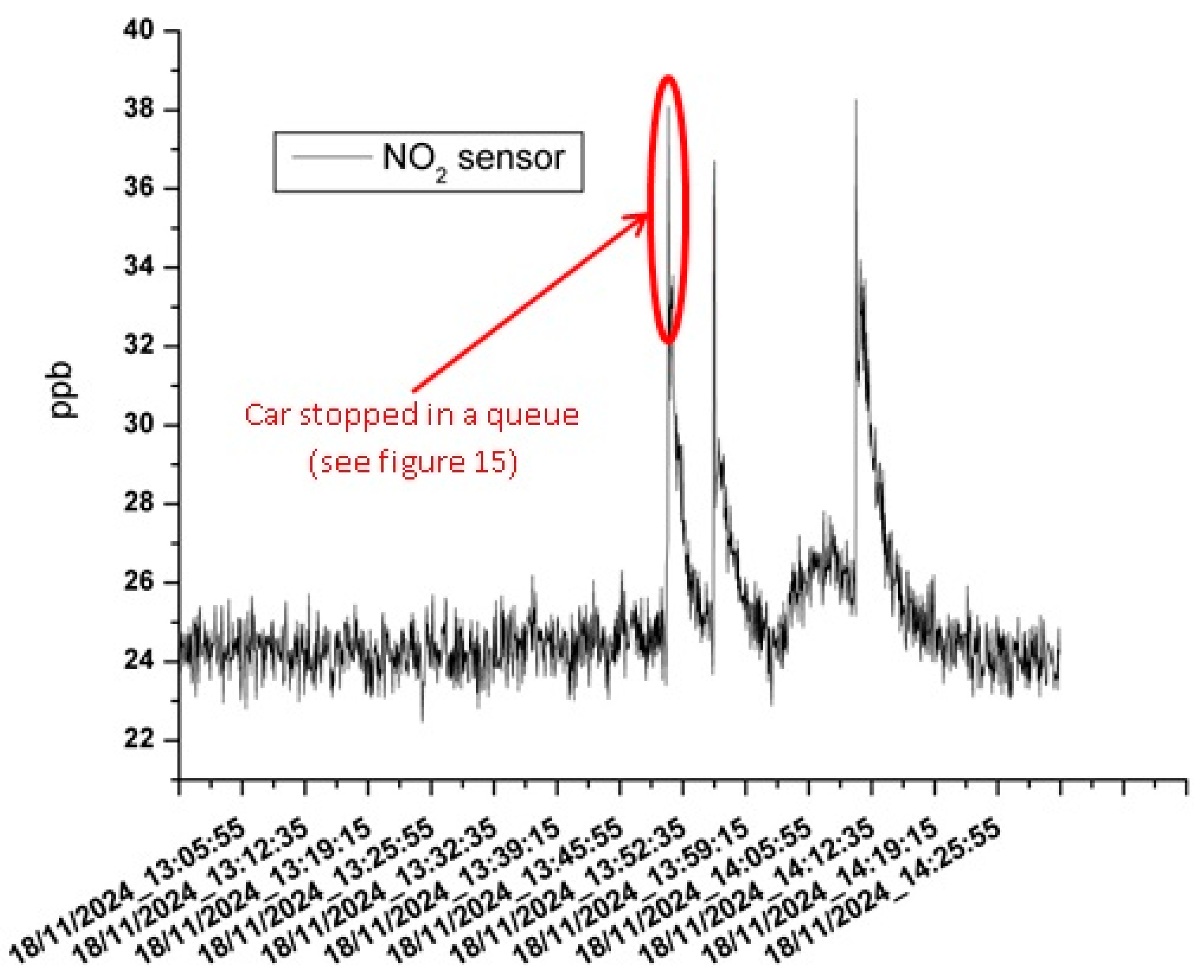
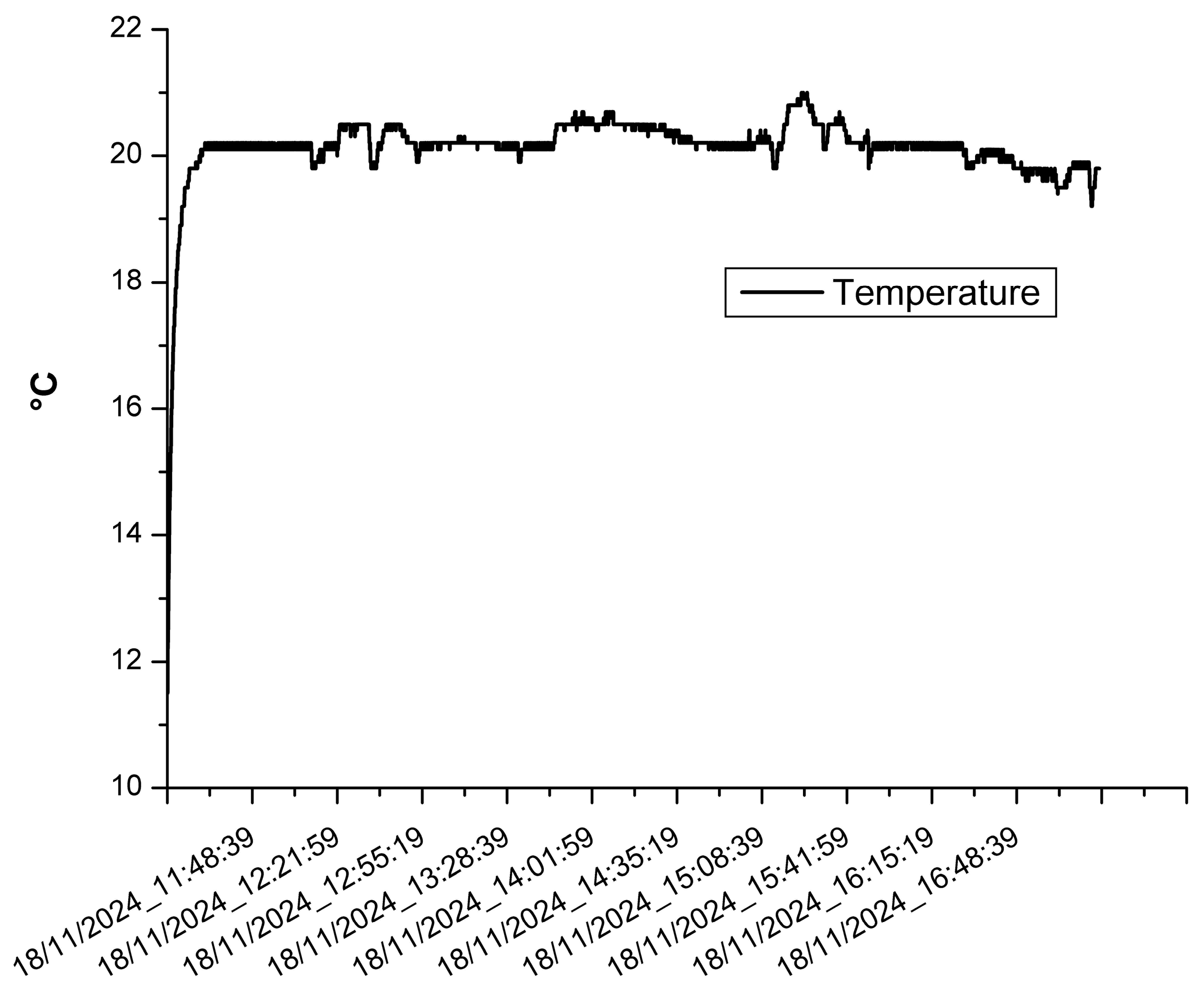
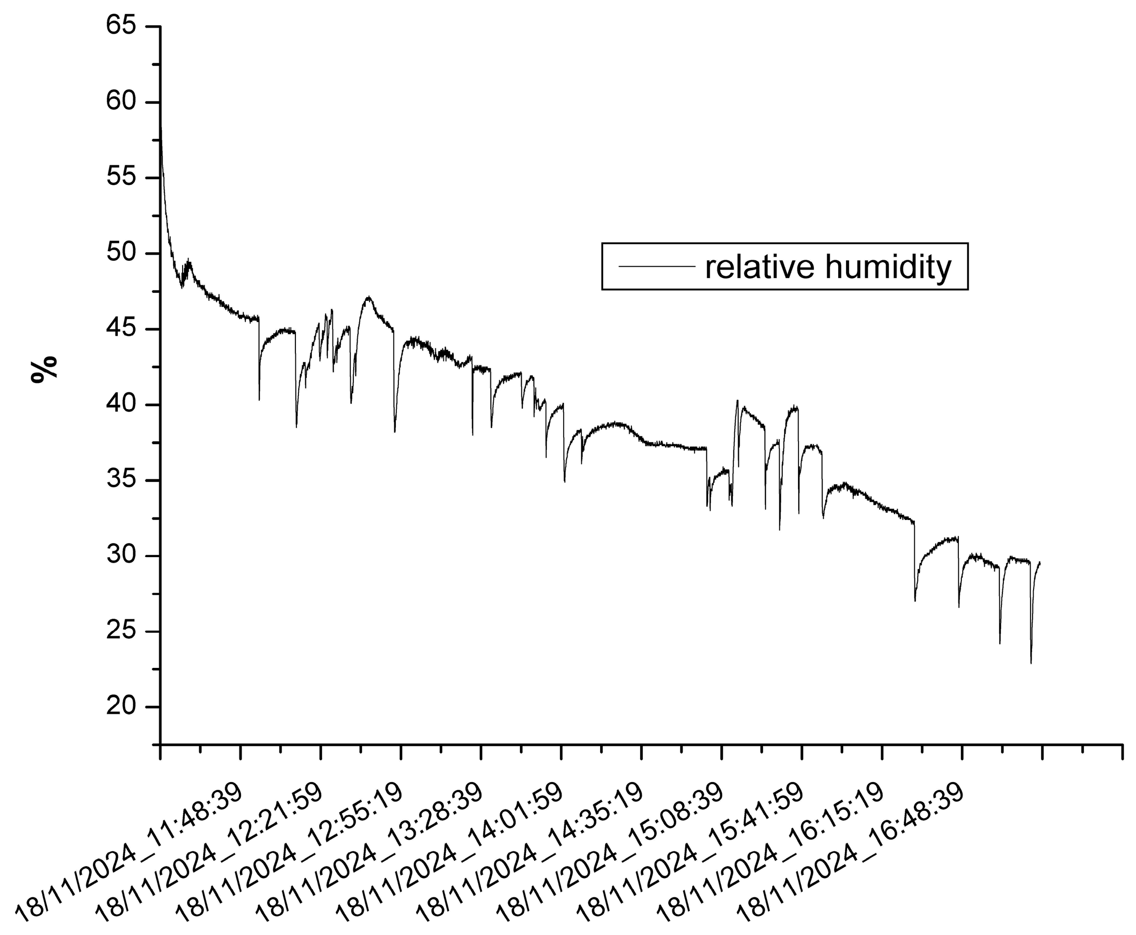
3.3. The Results of the Mobile Measurements

The mobile measurements were carried out by making a trip in a diesel fueled car during rush hour on urban and extra-urban roads. In this test, the monitor placed in the kitchen during the indoor experiment was used. The mobile measurements were performed on the 18 November 2024 and, by being mobile monitoring, the sampling rate of the monitor was set to 4 s, which is the fastest sampling rate possible for this device. Therefore, the resulting dataset was composed of 5486 measurements. The maximum value for the CO concentrations was equal to 8.3 ppm, while the maximum value for NO₂ concentrations was equal to 38 ppb. As regards to the temperature and relative humidity ranges, they were, respectively, from 11.5 °C to 21 °C and from 22.3% to 59.8%. The ranges of temperature and humidity are wider than the ones found during the apartment test, but if we consider the mean and median values for the temperature (respectively, equal to 20.1 °C and 20.2 °C), it can be seen that they are comparable with the values registered during the calibration phase. As concerns the humidity, we registered a continuous decrease in its values, which resulted in a mean value equal to 39% and a median value equal to 38.7%. The time series of these measurements are shown in Figure 13 and Figure 14, while Figure 15 highlights a moment in which we registered a spike in the NO₂ and CO concentrations due to a prolonged stop while we were waiting in a queue caused by heavy traffic. The trends of temperature and relative humidity measured in the car cabin are exposed, respectively, in Figure 16 and Figure 17.

4. Discussion

The calibration of the sensors for air quality monitoring is an important step for a good quality of data to be produced by the monitors. The scientific community has explored different calibration techniques that can be summarized in two big general categories: laboratory calibrations and on-field calibrations [5,8]. Laboratory calibrations are carried out in a protected environment, such as a laboratory, where the device to calibrate is placed into a test chamber in which all the variables affecting the sensor response are under control and also the interfering gases can be excluded. On the contrary, on-field calibrations are performed in the place where the sensor will be deployed in co-location with reference instrumentations [6]. In this second case, temperature, relative humidity, and interfering gases cannot be controlled, but their effects are taken into account in the conversion law which is to be applied to the sensor under calibration. Both of the two approaches have advantages and disadvantages, but in general, calibration in a laboratory provides better performance indicator values in terms of R² [5,8,12].

In the review proposed by Kang et al. [12], it has been found that, in the case of CO and NO₂ sensors, laboratory evaluations produced R² values ranging between 0.99 and 1. The values found during the calibration of the sensors used for this work, ranging from 0.995 to 0.999, are in line with the study carried out by Kang.

Other researchers have performed laboratory calibration of electrochemical sensors for their work. Zimmerman et al. [27] used nine CO-B4 sensors and fourteen NO2-B43F sensors to implement several devices to monitor CO and NO₂. For the laboratory calibrations they used the multivariate linear regression technique to find the conversion law. After the calibration process, they found an average R² equal to 0.98 for both of the sensor types, and an average value for MAE equal to 132 ppb in the case of the CO-B4 sensor and 35 ppb in the case of the NO2-B43F sensor. In this study, similar values were found for both of the performance indicators.

Castell et al. [8] evaluated in their study 24 units of the same monitor model (the v3.5 type) produced by AQmesh for measuring CO, NO₂, NO, and O₃. These monitors were based on the CO-B4 sensor for CO measurements and on the NO2B42 sensor for NO₂ measurements, a model very similar to the NO2-B43F considered in our study. Two of the twenty-four units were calibrated in the laboratory and the linear regression technique was used for this purpose. After the calibration process, they found R² values equal to 0.99 for both sensor models, which is comparable with the values found after the calibration performed for our study.

Castell et al., along with many other researcher groups, highlighted that meteorological conditions influence the response of electrochemical sensors. More specifically, the relative humidity, and more heavily the temperature, can play a significant role in determining the final sensor outputs. For this reason, it is important to take into account their variations in the conversion law, or alternatively, to deploy them in environments where temperature and humidity have limited variations.

In our preliminary study we did not include these variables in the conversion law, but we designed the tests by reproducing the laboratory conditions. During the laboratory calibrations the temperature ranged from 18.6 °C to 21.2 °C while the relative humidity ranged from 39.5% to 53.7%. By examining the documents and the datasheets published by the manufacturer of the sensors, these ranges do not have a remarkable influence on the sensor response due to the fact that they are limited enough. As desired, these values were comparable with the ones registered during the indoor experiment (16.7 °C to 21.2 °C for the temperature and 38.8% to 54.2% for the humidity).

As concerns the mobile measurements performed in the car cabin, the ranges of temperature and humidity are both wider (from 11.5 °C to 21 °C for the temperature and from 22.3% to 59.8% for the humidity) than the ones measured during the laboratory calibration. The reason for this result can be explained by considering that, before starting the experiment, the car used for this test was parked in an underground carpark, where environmental conditions were different from the ones planned for the experiment. The measurements started when the car was in the carpark, and the car conditioning system was set to 20 °C as soon as the car was started. As you can see in Figure 16, the temperature values very quickly reached their planned level, and subsequently they did not move out of the range measured during the calibration for the whole duration of the experiment. All these elements explain the trend of the temperature exposed in Figure 16. By considering that the temperature was out of the range measured during the calibration for a very short time, we can judge the measures carried out through this test to be reliable. Similar considerations can be drawn in the case of the relative humidity, even though its trend showed that the calibration range was reached more gradually (see Figure 17).

In the indoor experiment, the concentrations of CO and NO₂ gases were measured during the everyday activities which typically take place in an apartment: cooking, cleaning, or smoking. The results highlight that the peaks of gas emissions (see Figure 11 and Figure 12) were registered mainly during smoking and cleaning. While it was expected that cigarette smoke can emit CO or NO₂ gases, to a certain extent, it was unexpected that peaks of concentrations of CO or NO₂ can be measured also when some household cleaning products are used for cleaning activities. It is very likely, or better we can surely consider, that those products did not emit CO or NO₂, but rather some interfering gases or VOCs (volatile organic compounds), even though we could not identify which type of them could be. Another important element of this experiment is given by the similar trends registered by both the monitors, in addition to the fact that the monitor placed in the kitchen measured concentrations higher than the one placed in the living room. This is explained by the position of pollutant sources, which were all located in the kitchen, and also by considering that the sliding door between the living room and the kitchen was always kept open. The maximum value of NO₂ concentration was 64ppb, which is way lower than the WHO limit set to 106 ppb (1 h average) in the 2023 air quality guidelines [44]. As regarding the CO concentrations, the same considerations can be made as the maximum concentration measured in the apartment was equal to 12.3 ppm, which is lower than the WHO limit equal to 26 ppm.

As concerns the mobile measurements carried out in the car cabin, we noted that the peaks of CO and NO₂ occurred when the car was stopped in traffic very close to other vehicles, forming the queue as shown in Figure 15. The rapid increase in gas concentrations and their slower decrease shown in Figure 13 and Figure 14 are explained by the car ventilation being set to the minimum in conjunction with the car windows being kept closed. It was necessary to keep them closed to avoid excessive variations in temperature and humidity in the car cabin. During this experiment the WHO limits were not exceeded as the maximum concentration for NO₂ was equal to 38 ppb, whilst we recorded 8.3 ppm for the CO.

5. Conclusions

A new device called DSNasus for monitoring personal exposure to air pollutant gases has been designed and implemented. For its operation, a smartphone device and electrochemical gas sensors by Alphasense are needed. In this preliminary work, its functionalities have been tested by performing two experiments. The first one was aimed at forming a little indoor network composed of two monitors measuring CO and NO₂ concentrations and a smartphone acting as a hub for the measure records. In the second experiment, mobile measurements were performed in a car cabin during a trip through urban and extra-urban roads. Considering the results of both the experiments and considering that in some environments interfering gases or volatile compounds can be still an issue, we can conclude that this device can be used as a personal air quality indicator tool rather than a tool for assessing the personal exposure to specific pollutant gases.

References

1. Gumy, S.; Prüss-Üstün, A. Ambient Air Pollution: A Global Assessment of Exposure and Burden of Disease; WHO: Geneva, Switzerland, 2016.
2. European Commission. Indoor Air Pollution: New EU Research Reveals Higher Risks than Previously Thought. 2017. Available online: https://ec.europa.eu/commission/presscorner/detail/en/IP_03_1278 (accessed on 10 December 2024).
3. WHO. How Air Pollution Is Destroying Our Health. 2018. Available online: https://www.who.int/news-room/spotlight/how-air-pollution-is-destroying-our-health (accessed on 10 December 2024).
4. EPA. The Inside Story: A Guide to Indoor Air Quality. 2017. Available online: https://www.epa.gov/indoor-air-quality-iaq/inside-story-guide-indoor-air-quality (accessed on 10 December 2024).
5. Karagulian, F.; Barbiere, M.; Kotsev, A.; Spinelle, L.; Gerboles, M.; Lagler, F.; Redon, N.; Crunaire, S.; Borowiak, A. Review of the Performance of Low-Cost Sensors for Air Quality Monitoring. Atmosphere 2019, 10, 506. [Google Scholar] [CrossRef]
6. Spinelle, L.; Gerboles, M.; Villani, M.G.; Aleixandre, M.; Bonavitacola, F. Field calibration of a cluster of low-cost commercially available sensors for air quality monitoring. Part B: NO, CO and CO2. Sens. Actuators B Chem. 2017, 238, 706–715. [Google Scholar] [CrossRef]
7. Mead, M.I.; Popoola, O.A.M.; Stewart, G.B.; Landshoff, P.; Calleja, M.; Hayes, M.; Baldovi, J.J.; McLeod, M.W.; Hodgson, T.F.; Dicks, J.; et al. The use of electrochemical sensors for monitoring urban air quality in low-cost, high-density networks. Atmos. Environ. 2013, 70, 186–203. [Google Scholar] [CrossRef]
8. Castell, N.; Dauge, F.R.; Schneider, P.; Vogt, M.; Lerner, U.; Fishbain, B.; Broday, D.; Bartonova, A. Can commercial low-cost sensor platforms contribute to air quality monitoring and exposure estimates? Environ. Int. 2017, 99, 293–302. [Google Scholar] [CrossRef]
9. McKercher, G.R.; Salmond, J.A.; Vanos, J.K. Characteristics and applications of small, portable gaseous air pollution monitors. Environ. Pollut. 2016, 223, 102–110. [Google Scholar] [CrossRef] [PubMed]
10. Kumar, P.; Morawska, L.; Martani, C.; Biskos, G.; Neophytou, M.; Di Sabatino, S.; Bell, M.; Norford, L.; Britter, R. The rise of low-cost sensing for managing air pollution in cities. Environ. Int. 2015, 75, 199–205. [Google Scholar] [CrossRef]
11. Snyder, E.G.; Watkins, T.H.; Solomon, P.A.; Thoma, E.D.; Williams, R.W.; Hagler, G.S.; Shelow, D.; Hindin, D.A.; Kilaru, V.J.; Preuss, P.W. The Changing Paradigm of Air Pollution Monitoring. Environ. Sci. Technol. 2013, 47, 11369–11377. [Google Scholar] [CrossRef]
12. Kang, Y.; Aye, L.; Ngo, T.D.; Zhou, J. Performance evaluation of low-cost air quality sensors: A review. Sci. Total Environ. 2022, 818, 151769. [Google Scholar] [CrossRef] [PubMed]
13. Suriano, D. SentinAir system software: A flexible tool for data acquisition from heterogeneous sensors and devices. SoftwareX 2020, 12, 100589. [Google Scholar] [CrossRef]
14. Tryner, J.; Phillips, M.; Quinn, C.; Neymark, G.; Wilson, A.; Jathar, S.H.; Carter, E.; Volckens, J. Design and testing of a low-cost sensor and sampling platform for indoor air quality. Build. Environ. 2021, 206, 108398. [Google Scholar] [CrossRef]
15. Jo, J.; Jo, B.; Kim, J.; Kim, S.; Han, W. Development of an IoT-Based Indoor Air Quality Monitoring Platform. J. Sens. 2020, 2020, 8749764. [Google Scholar] [CrossRef]
16. Mandal, D.; Banerjee, S. Surface Acoustic Wave (SAW) Sensors: Physics, Materials, and Applications. Sensors 2022, 22, 820. [Google Scholar] [CrossRef]
17. Han, T.; Nag, A.; Mukhopadhyay, S.C.; Xu, Y. Carbon nanotubes and its gas-sensing applications: A review. Sens. Actuators A Phys. 2019, 291, 107–143. [Google Scholar] [CrossRef]
18. Sayahi, T.; Garff, A.; Quah, T.; Lê, K.; Becnel, T.; Powell, K.M.; Gaillardon, P.E.; Butterfield, A.E.; Kelly, K.E. Long term calibration models to estimate ozone concentrations with a metal oxide sensor. Environ. Pollut. 2020, 267, 1–10. [Google Scholar] [CrossRef] [PubMed]
19. Velasco, A.; Ferrero, R.; Gandino, F.; Montrucchio, B.; Rebaudengo, M. A mobile and low-cost system for environmental monitoring: A case study. Sensors 2016, 16, 710. [Google Scholar] [CrossRef]
20. Spinelle, L.; Gerboles, M.; Villani, M.G.; Aleixandre, M.; Bonavitacola, F. Field calibration of a cluster of low-cost available sensors for air quality monitoring. Part A: Ozone and nitrogen dioxide. Sens. Actuators B Chem. 2015, 215, 249–257. [Google Scholar] [CrossRef]
21. Mijling, B.; Jiang, Q.; De Jonge, D.; Bocconi, S. Field calibration of electrochemical NO2 sensors in a citizen science context. Atmos. Meas. Tech. 2018, 11, 1297–1312. [Google Scholar] [CrossRef]
22. Hagan, D.H.; Isaacman-VanWertz, G.; Franklin, J.P.; Wallace, L.M.; Kocar, B.D.; Heald, C.L.; Kroll, J.H. Calibration and assessment of electrochemical air quality sensors by co-location with regulatory-grade instruments. Atmos. Meas. Tech. 2018, 11, 315–328. [Google Scholar] [CrossRef]
23. Demanega, I.; Mujan, I.; Singer, B.C.; Anđelković, A.S.; Babich, F.; Licina, D. Performance assessment of low-cost environmental monitors and single sensors under variable indoor air quality and thermal conditions. Build. Environ. 2021, 187, 107415. [Google Scholar] [CrossRef]
24. Wei, P.; Sun, L.; Anand, A.; Zhang, Q.; Huixin, Z.; Deng, Z.; Wang, Y.; Ning, Z. Development and evaluation of a robust temperature sensitive algorithm for long term NO2 gas sensor network data correction. Atmos. Environ. 2020, 230, 1–10. [Google Scholar] [CrossRef]
25. Wei, P.; Ning, Z.; Ye, S.; Sun, L.; Yang, F.; Wong, K.C.; Westerdahl, D.; Louie, P.K.K. Impact Analysis of Temperature and Humidity Conditions on Electrochemical Sensor Response in Ambient Air Quality Monitoring. Sensors 2018, 18, 59. [Google Scholar] [CrossRef] [PubMed]
26. Smith, K.R.; Edwards, P.M.; Ivatt, P.D.; Lee, J.D.; Squires, F.; Dai, C.; Peltier, R.E.; Evans, M.J.; Sun, Y.; Lewis, A.C. An improved low–power measurement of ambient NO2 and O3 combining electrochemical sensor clusters and machine learning. Atmos. Meas. Tech. 2019, 12, 1325–1336. [Google Scholar] [CrossRef]
27. Zimmerman, N.; Presto, A.A.; Kumar, S.P.N.; Gu, J.; Hauryliuk, A.; Robinson, E.S.; Robinson, A.L.; Subramanian, R. A machine learning calibration model using random forests to improve sensor performance for lower-cost air quality monitoring. Atmos. Meas. Tech. 2018, 11, 291–313. [Google Scholar] [CrossRef]
28. Hossain, M.; Saffell, J.; Baron, R. Differentiating NO2 and O3 at low cost air quality amperometric gas sensors. ACS Sens. 2016, 1, 1291–1294. [Google Scholar] [CrossRef]
29. Bigi, A.; Mueller, M.; Grange, S.K.; Ghermandi, G.; Hueglin, C. Performance of NO, NO2 low cost sensors and three calibration approaches within a real world application. Atmos. Meas. Tech. 2018, 11, 3717–3735. [Google Scholar] [CrossRef]
30. Suriano, D.; Penza, M. Assessment of the Performance of a Low-Cost Air Quality Monitor in an Indoor Environment through Different Calibration Models. Atmosphere 2022, 13, 567. [Google Scholar] [CrossRef]
31. Cordero, J.M.; Borge, R.; Narros, A. Using statistical methods to carry out in field calibrations of low cost air quality sensors. Sens. Actuators B Chem. 2018, 267, 245–254. [Google Scholar] [CrossRef]
32. Trizio, L.; Brattoli, M.; De Gennaro, G.; Suriano, D.; Rossi, R.; Alvisi, M.; Cassano, G.; Pfister, V.; Penza, M. Application of artificial neural networks to a gas sensor-array database for environmental monitoring. In Sensors and Microsystems; Springer: Boston, MA, USA, 2012; pp. 139–144. [Google Scholar]
33. Cross, E.S.; Williams, L.R.; Lewis, D.K.; Magoon, G.R.; Onasch, T.B.; Kaminsky, M.L.; Worsnop, D.R.; Jayne, J.T. Use of electrochemical sensors for measurement of air pollution: Correcting interference response and validating measurements. Atmos. Meas. Tech. 2017, 10, 3575–3588. [Google Scholar] [CrossRef]
34. Liang, Y.; Wu, C.; Jiang, S.; Li, Y.J.; Wu, D.; Li, M.; Cheng, P.; Yang, W.; Cheng, C.; Li, L.; et al. Field comparison of electrochemical gas sensor data correction algorithms for ambient air measurements. Sens. Actuators B Chem. 2021, 327, 1–13. [Google Scholar] [CrossRef]
35. Han, P.; Mei, H.; Liu, D.; Zeng, N.; Tang, X.; Wang, Y.; Pan, Y. Calibrations of Low-Cost Air Pollution Monitoring Sensors for CO, NO2, O3, and SO2. Sensors 2021, 21, 256. [Google Scholar] [CrossRef]
36. Dai, Y.; Mazzeo, A.; Zhong, J.; Cai, X.; Mele, B.; Toscano, D.; Murena, F.; MacKenzie, A.R. Modelling of Deep Street Canyon Air Pollution Chemistry and Transport: A Wintertime Naples Case Study. Atmosphere 2023, 14, 1385. [Google Scholar] [CrossRef]
37. Mendoza, D.L.; Benney, T.M.; Boll, S. Long-term analysis of the relationships between indoor and outdoor fine particulate pollution: A case study using research grade sensors. Sci. Total Environ. 2021, 776, 145778. [Google Scholar] [CrossRef] [PubMed]
38. Baron, R.; Saffell, J. Amperometric gas sensors as a low cost emerging technology platform for air quality monitoring applications: A review. ACS Sens. 2017, 2, 1553–1566. [Google Scholar] [CrossRef] [PubMed]
39. Najafi, P.; Ghaemi, A. Chemiresistor gas sensors: Design, Challenges, and Strategies: A comprehensive review. Chem. Eng. J. 2024, 498, 154999. [Google Scholar] [CrossRef]
40. NO2-B43F Datasheet. Available online: https://ametekcdn.azureedge.net/mediafiles/project/oneweb/oneweb/alphasense/products/datasheets/alphasense_no2-b43f_datasheet_en_4.pdf (accessed on 27 March 2025).
41. CO2-B4 Datasheet. Available online: https://ametekcdn.azureedge.net/mediafiles/project/oneweb/oneweb/alphasense/products/datasheets/alphasense_co-b4_datasheet_en_2.pdf (accessed on 27 March 2025).
42. Suriano, D. Design and Development of an Electronic Board for Supporting the Operation of Electrochemical Gas Sensors. Hardware 2024, 2, 173–189. [Google Scholar] [CrossRef]
43. Alphasense Ozone Sensors. Available online: https://www.alphasense.com/products/view-by-target-gas/ozone-sensors-o3 (accessed on 27 March 2025).
44. WHO. World Health Organization (WHO) Air Quality Guidelines (AQGs) and Estimated Reference Levels (RLs). Available online: https://www.eea.europa.eu/publications/status-of-air-quality-in-Europe-2022/europes-air-quality-status-2022/world-health-organization-who-air (accessed on 27 March 2025).
Figure 1. On the left of the figure we can find two monitors, DSnasus, implemented in our laboratory, while on the right there is the smartphone device used for the experiments showing the App running. The sizes of the DSnasus monitors are 17 cm × 8.5 cm.
Chemosensors 13 00189 g001
Figure 2. A representation of the NO2-B43F sensor. The CO-B4 sensor has same size and features.
Chemosensors 13 00189 g002
Figure 3. A system composed of smartphone devices and more DSnasus’s can be used to form multiple star-shaped networks based on Bluetooth connections, where the smartphone is the center, or hub, to which the measures converge, while the DSnasus monitors are the branches providing the measures.
Chemosensors 13 00189 g003
Figure 4. The apartment map, its size, and the position of the two monitors forming the monitoring network. The height of the apartment walls is 2.75 m.
Chemosensors 13 00189 g004
Figure 5. The position of the monitor placed in the kitchen (monitor 1) (a), and the monitor placed in the living room (monitor 2) (b), as reported also in Figure 4.
Chemosensors 13 00189 g005
Figure 6. The monitor used for mobile measurements arranged on the car dashboard by using a standard smartphone holder.
Chemosensors 13 00189 g006
Figure 7. The calibration of the first CO-B4 sensor, herein denoted as CO(1), and the CO concentrations read by the reference instruments.
Chemosensors 13 00189 g007
Figure 8. The calibration of the second CO-B4 sensor, herein denoted as CO(2), and the CO concentrations read by the reference instruments.
Chemosensors 13 00189 g008
Figure 9. The calibration of the first NO2-B43F sensor, herein denoted as NO2(1), and the NO2 concentrations read by the reference instruments.
Chemosensors 13 00189 g009
Figure 10. The calibration of the second NO2-B43F sensor, herein denoted as NO2(2), and the NO2 concentrations read by the reference instruments.
Chemosensors 13 00189 g010
Figure 11. The CO concentrations measured by the CO(1) sensor placed in the apartment kitchen and the ones measured by the CO(2) sensor placed in the living room.
Chemosensors 13 00189 g011
Figure 12. The NO2 concentrations measured by the NO2(1) sensor placed in the apartment kitchen and the ones measured by the NO2(2) sensor placed in the living room.
Chemosensors 13 00189 g012
Figure 13. The time series of the CO concentrations measured in the mobile measurement test. In this figure is shown the spike registered during a stop in a queue caused by heavy traffic caught in Figure 15.
Chemosensors 13 00189 g013
Figure 14. The time series of the NO2 concentrations measured in the mobile measurement test. In this figure is shown the spike registered during a stop in a queue caused by heavy traffic caught in Figure 15.
Chemosensors 13 00189 g014
Figure 15. This figure shows the car stopping in a queue caused by heavy traffic, in which a remarkable peak of CO and NO2 concentrations was registered by the monitor arranged on the car dashboard.
Chemosensors 13 00189 g015
Figure 16. The time series of the temperature measured in the car cabin.
Chemosensors 13 00189 g016
Figure 17. The time series of the relative humidity measured in the car cabin.
Chemosensors 13 00189 g017