Analytical Study of the Detection Model for Sulphate Saline Soil Based on Mid-Infrared Spectrometry

Abstract

High soil sulfate levels can inhibit crop growth and accelerate concrete infrastructure degradation, highlighting the critical importance of rapid and accurate sulfate content determination. Nevertheless, conventional analytical techniques are laborious and intricate, and delays in processing may result in alterations to the material, owing to oxidation. We recognized the accuracy, reproducibility, and non-invasiveness of mid-infrared (MIR) spectroscopy as a rapid and straightforward technique for soil analysis. In this study, soil samples were collected from two depths (0–20 cm and 20–40 cm) across three regions in China: the arid northwestern region, the cold-temperate northeastern zone, and the subtropical southwestern region. One group was mixed with Na₂SO₄ (a readily soluble salt) at mass fractions ranging from 0.1% to 7%, while the other group was mixed with FeS₂ (a sulfide) at mass fractions ranging from 1% to 70%. This study aimed to develop a mid-infrared spectroscopy-based method for analyzing soluble sulfate and sulfide in soil. Three chemometric methods were evaluated: partial least squares regression (PLSR), principal component regression (PCR), and multivariate linear regression (MLR). Results showed that the MLR model provided superior predictive performance. For the 20–40 cm sodium sulfate-mixed soil from the arid northwestern region, the MLR model exhibited the best performance with an Rp² of 0.9535, an RMSEP of 0.0030, an RPD of 4.96, and an RPIQ of 6.26. For the 20–40 cm iron disulfide-mixed soil from the cold-temperate northeastern region, the MLR model demonstrated superior results with Rp², RMSEP, RPD, and RPIQ values of 0.9590, 0.042, 5.97, and 10.94, respectively. For the 0–20 cm iron disulfide-mixed soil from the subtropical southwestern region, the MLR model achieved the best performance with an Rp² of 0.9848, an RMSEP of 0.0025, an RPD of 14.20, and an RPIQ of 25.48. Despite regional variations in soil properties, this study successfully predicted sulfate and sulfide contents in soils from diverse areas using mid-infrared spectroscopy combined with appropriate chemometric methods. This approach provides reliable technical support for soil sulfate detection and offers significant practical value for soil assessment in both agricultural production and engineering construction.

1. Introduction

Soil salinization happens when salts that are easily dissolved in groundwater or soil rise to the surface with capillary water. As the water evaporates, the salts build up on top of the soil [1]. Soil salinization is a serious environmental danger that poses a significant threat to the land, and saline soils in China have a wide distribution, large size, and different varieties, with a total area of approximately 100 million hectares [2]. Elevated sulfate levels in soils, salt lakes, and karst regions can result in diminished agricultural productivity due to reduced soil fertility and the hastened degradation of concrete structures in engineering and construction, adversely affecting human life [3,4]. The issue of soil salinization has garnered significant attention in numerous countries [5,6]. Consequently, monitoring and quantifying the sulfate concentration in soil is crucial.

Freely soluble salts constitute a significant element of salty soils. They are a primary determinant of crop growth, particularly in arid and semi-arid locations, where water-soluble chloride ions and sulfates, notably SO₄²⁻, serve as critical indicators of soil salinity. Moreover, acid sulfate soils encompass sulfuric acid or soils and sediments capable of generating sulfuric acid, potentially impacting many soil parameters significantly [7]. Soils or sediments rich in pyrite are stable in reducing conditions; nevertheless, upon exposure to oxygen, sulfides (mainly pyrite) generate sulfuric acid [8], represented by the following reaction, Equation (1):

FeS₂ + 15/4O₂ + 7/2H₂O → Fe(OH)₃ + 2SO₄²⁻ + 4H⁺

(1)

The synthesis of sulfuric acid from sulfur-containing materials releases soluble iron, aluminum, and other heavy metals, adversely affecting the environment. Consequently, the precise and reliable monitoring of sulfate content is essential for judicious fertilizer application and precision agriculture.

Conventional laboratory chemical analysis methods predominantly assess soil sulfate concentration; however, this approach is hindered by prolonged cycle times and elevated costs [9]. In recent years, infrared spectroscopy (IR) has gained prominence owing to its non-destructive nature, quick analysis, and low sample preparation requirements [10]. Infrared spectroscopy relies on the absorption of photons by molecular bonds. Infrared spectroscopy is based on the phenomenon of molecular bonds absorbing photons, which follows Beer–Lambert’s law, that is, the degree of absorption of infrared light by a sample is directly proportional to the sample concentration and optical pathlength, and the molecules in the sample selectively absorb infrared light energy at a specific frequency according to the vibrational mode of their chemical bonds (such as stretching vibration, bending vibration, etc.) [11]. Barra et al. [12] discovered that mid-infrared and near-infrared spectroscopy techniques are effective at precisely predicting specific features. When it came to estimating most soil indicators, the mid-infrared spectroscopy technique outperformed the near-infrared spectroscopy method. Mid-infrared reflectance spectroscopy enables the more accurate, precise, and focused characterization of diverse minerals and organic soils [13]. The advantage of infrared (IR) technology is its abundance of information, yet this also constrains its accuracy due to considerable irrelevant data [14]. When a model is built with the full spectrum as an input variable, irrelevant information is introduced, which can degrade the prediction performance of the model. Consequently, selecting variables before modeling is an excellent strategy to enhance the model’s prediction performance [15].

Zhang et al. [16] focused on remote sensing to detect salinity variations at different depths. The researchers established quantitative relationship models between surface spectral signatures and soil salt content and explored advanced techniques for monitoring vertical salinity profiles. The traditional measurements of surface soil salinity (0–5 cm) are insufficient for comprehensively evaluating the salt conditions in deeper soil layers, as soil salts migrate through the soil profile during cultivation and irrigation processes. Leila Lotfollahi et al. [17] employed mid-infrared and visible–near-infrared spectroscopy to predict soil salinity–alkalinity indicators, such as the sodium adsorption ratio (SAR) and exchangeable sodium ratio (ESR). The model performance was calibrated and evaluated using several key metrics, including the ratio of performance to deviation (RPD) and the coefficient of determination (R²). The research findings indicate that mid-infrared spectroscopy demonstrated superior accuracy and precision compared to near-infrared spectroscopy. J. Yin et al. [18] investigated the feasibility of infrared spectroscopy for predicting total nitrogen (TN) and total phosphorus (TP) concentrations in soil samples. The prediction performance of the spectra followed laboratory MIR > laboratory vis-NIR > in situ vis-NIR > in situ MIR. The performance of in situ MIR was relatively poor, mainly due to the fact that MIR was influenced more by the soil moisture. Francisco M. Canero et al. [19] enhanced modeling accuracy by integrating various preprocessing methods in a global dataset, including raw spectra, continuum removal, and multiplicative scatter correction. The PLSR models achieved prediction accuracies of 1.41 and 0.29 for soil organic matter and carbonates, respectively.

The above studies indicate that most researchers have focused on predicting labile salts [20] or organic matter [21,22] in soils, with little research on the prediction of specific inorganic compounds. This research gap is particularly concerning given that insoluble sulfides like pyrite (iron disulfide) undergo significant transformations when exposed to air and water, decomposing into iron oxides and sulfates that contribute to the formation of sulfate-rich saline soils. The corrosion of certain construction steels accelerates with prolonged exposure to environments with high sodium sulfate content, such as certain salt lakes. Therefore, developing a predictive model for sulfate levels based on sodium sulfate and iron disulfide concentrations represents an urgent research need.

In this study, three geographically distinct regions—Xinjiang, Heilongjiang, and Sichuan—were selected as the study areas with the following specific objectives: (1) identify region-specific pretreatment methods for soils at different depths, thereby overcoming the matrix interference effects that have compromised previous predictive models; (2) utilize soil spectral information by systematically examining the correlation between mid-infrared spectral features and sulfate and sulfide contents, enabling more accurate prediction than previously achieved; (3) compare the prediction accuracy of three models for quantitatively predicting the salt content in soils containing mixed sodium sulfate and iron disulfide, ultimately identifying the most suitable and specific methodological approach for each region.

2. Materials and Methods

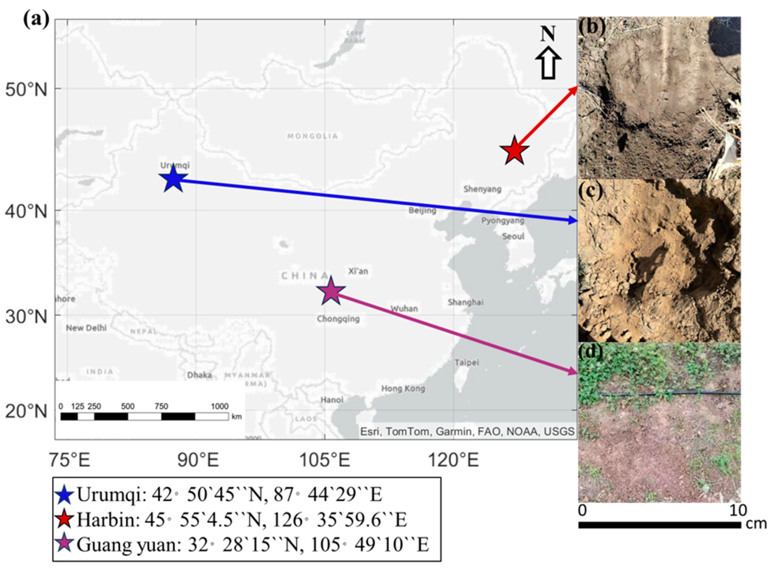
2.1. Spiking Treatments and Sample Preparation

This study collected three groups of soil samples, YS, BS, and PS, from Xinjiang in the northwestern arid zone, Heilongjiang Province in the northeastern cold-temperate zone, and Sichuan Province in the southwestern subtropical zone, at two depths of 0–20 cm and 20–40 cm, respectively, and the sampling points are shown in Figure 1. According to the Chinese soil classification system, they belong to the desert soil class, containing a certain mix of fine sand, wonderful sand, and clayey grains, clayey black soil with intense swelling, shrinking, and disturbing characteristics, and mountain brown soil developed on calcium carbonate-rich purplish-red sandstone and shale, respectively. As shown in

Table 1. Detailed information on sampling locations and soil properties.

Abbreviation	Source	Latitude and Longitude	Depths/cm	SO42−/mg/kg	Cl−/mg/kg	pH
YS02	Urumqi City, Xinjiang Uyghur Autonomous Region, China	42°50′45″ N 87°44′29″ E	0–20	99.40	51.2	9.41
YS24			20–40	129.21	64.82	9.66
BS02	Harbin, Heilongjiang Province, China	45°55′4.5″ N 126°35′59.6″ E	0–20	93.78	19.84	7.20
BS24			20–40	104.32	36.82	7.01
PS02	Guang Yuan, Sichuan Province, China	32°28′15″ N 105°49′10″ E	0–20	53.23	16.44	8.55
PS24			20–40	50.02	14.13	8.65

, the samples were air-dried, ground, and passed through a sieve with a pore size of 0.25 mm.

We prepared two methods for artificially adding samples to six groups of washed soil samples. Soils were dried after immersion in the Na₂SO₄ (Greagent, 99.0%) solution in the mass range of 0.1–7%, recorded as the N series; soils were mechanically mixed with FeS₂ (Adamas, 99.99%) in the mass range of 1–70%, recorded as the F series. Forty-five different concentrations were added to each group of soil, for a total of 45 × 6 × 2 = 540 samples. A list of all the mixed soil samples is in Supplementary Table S1. The samples were thoroughly ground in an agate mortar during spiking to ensure homogeneous mixing. The content of labile salts in the soil was determined by ion chromatography (Dionex Aquion, Thermo Fisher Scientific Inc., Waltham, MA, USA), and the soil pH was determined by a pH meter. The soil-to-water suspension ratio was 1:2.5. Ten grams of the soil sample was mixed with 25 milliliters of deionized water, shaken for 30 min in an oscillator, and then allowed to settle for 30 min before measurement. Since FeS₂ is susceptible to oxidative decomposition in air, it was stored in an inert gas, and Na₂SO₄ was placed in a medicine cabinet at room temperature and used directly.

2.2. Data Preprocessing and Spectral Measurements

The infrared spectra of soil samples were obtained using a Fourier Transform Infrared (FTIR) spectrometer (Great 10, CK Ruijie Technology Co., Tianjin, China) equipped with a mid-infrared reflectance device. Spectral data were collected across the wavenumber range of 4000–399 cm⁻¹. Before conducting the spectral analysis, background spectra were recorded and subtracted from an air background to reduce the influence of carbon dioxide and water. The soil’s infrared spectra were determined by the potassium bromide press method. The soil infrared spectrum was determined by the potassium bromide tablet method, the KBr (Adamas, 99.9%+, SP) dried at 150 °C for 1 h, and the soil was weighed with a universal balance instrument (FA2104B, Shanghai Yue Ping Scientific Instrument Co., Shanghai, China) to weigh 0.004 g of soil and 0.4 g of KBr. The mixture was mixed in a ratio of 1:100, placed in an onyx mortar, and fully ground for 30 s to ensure that the soil and the KBr were mixed homogeneously.

Since the thickness of the pressed film would lead to different degrees of infrared light penetration, the ground soil samples were quantitatively weighed at 0.1000–0.1010 g, transferred to the pressed film device and filled uniformly, and then pressed in the pressed film machine with a pressure of 14 MPa for 30 s. The thickness of the pressed film was about 1 mm and translucent, and the samples were uniformly distributed inside the KBr. The wavelength was used as a variable to find the absorbance variance of the mid-infrared spectra of the soil samples at each wavelength to find the optimal testing conditions for the spectra, with the parameters of resolution at 32 cm⁻¹ and the number of scans at 32, and the average spectra were obtained by testing each sample three times. The spectra were imported into the Unscrambler software (UnscramblerX-V10.4, CAMO, Oslo, Norway) for multivariate modeling analysis. The spectra are shown in Figure 2. The spectra of all mixed soils are shown in Supplementary Figures S1–S3.

Preprocessing serves as a fundamental component in the majority of spectroscopic investigations. The selection of an appropriate preprocessing method is contingent upon the specific characteristics of the data being examined. To ensure effective preprocessing, this study meticulously selected six distinct preprocessing techniques for a comparative analysis of spectroscopically acquired data. These methods are as follows:

(1)

Savitzky–Golay filtering (SG)

SG utilizes partial least squares fitting coefficients as a corresponding function of the numerical method to modify the processing of the original spectra when applying the convolutional smoothing technique. Additionally, a polynomial function is employed to perform polynomial partial least squares fitting on the data associated with the moving window. This approach enhances the clarity of the centroid’s center through the weighted average method [23].

(2)

Baseline

Baseline correction removes baseline shifts or drifts caused by the instrument, sample container, or other factors to ensure that the spectra respond to the properties of the sample itself [24]. The baseline correction method chosen is baseline offset, which corrects for the vertical shift across the spectrum by subtracting the value of a point or region. The offset will be calculated based on the entire spectral range in this setting.

(3)

Standard normal variate transform (SNV)

SNV centralizes and standardizes each spectrum independently so that each spectrum has zero mean and unit standard deviation. This decreases light scattering variations induced by sample physical properties including particle size and surface roughness [25].

(4)

Multiplicative scatter correction (MSC)

The MSC [26] can improve the signal-to-noise ratio of the original absorption spectrum and eliminate the linear scattering interference of the spectral data. Using the standard Full MSC method, using the mean spectrum as the reference spectrum, the specific process is as follows:

Calculate the average spectrum of the spectrum to be corrected:

$$\overline{A_{i,j}}={\displaystyle \frac{{\displaystyle \sum _{i=1}^n{A}_{i,j}}}{n}}$$

(2)

Perform the unary linear regression:

$$A_i=m_i\overline{A}+b_i$$

(3)

Obtain the MSC:

$$A_{i(MSC)}={\displaystyle \frac{(A_i-b_i)}{m_i}}$$

(4)

where $A$ is the calibration spectrum data matrix; $\overline{A_{i,j}}$ is the average spectral vector obtained by averaging the near-infrared spectrum at each wavelength point after the sample is smoothed by the SG algorithm; $m_i$ and $b_i$ are the relative offset coefficient and translation amount obtained after the unitary linear regression with the average spectrum, respectively.

(5)

Derivative

The derivative transform is capable of highlighting subtle spectral differences [27]. Its basic idea is to perform derivation operations on spectral data. The smooth part and the slow-changing part of the original spectral data are separated to highlight the fast-changing part. The derivative transformation can be divided into two forms: first-order derivative and second-order derivative. First-order derivatives can detect peaks and valleys in spectral data, while second-order derivatives can detect inflection points and slope changes.

2.3. Outliers Rejection and Identification of Key Wavelengths

In this paper, the two ways to improve the model accuracy are excluding outliers and weighted regression coefficients to select the characteristic wavelengths, and the three methods used to remove the outlier samples are Hotelling’s T², X-sample variance, and Q-residuals; Hotelling’s T² [28] is a multivariate statistic that measures the degree of outliers for each sample in a multidimensional space. The x-axis is the value of Hotelling’s T² statistic, with larger values indicating that the sample is farther away from the centroid and is likely to be a high-impact sample. The y-axis is the value of the F-residuals calculated. Larger values indicate that the point has a larger fitting error and may be an outlier or a sample that the model cannot fit effectively. The X-sample ANOVA [29] shows the proportion of variance explained by each sample in the X data (dependent variable data); the higher the variance explained, the more this sample plays an important role in the model and the better the fit in the model. The Q residual [30] measures the sum of squared residuals for a given sample, serving as an indicator of the difference between the actual observations and the model predictions projected outside of the model space. It assesses the degree to which the sample deviates from the established model. A significantly higher Q residual value for a sample, in comparison to others, may suggest that the sample is an outlier.

The weighted regression coefficients plot illustrates the trend of weighted regression coefficients (B/W) as a function of wavelength (X variable). The vertical axis is the magnitude of the regression coefficients, and the horizontal axis is the X variable. The configuration of each feature describes the significance of the standardized regression coefficient associated with that particular feature. Wavelet coefficients characterized by significant values of regression coefficients, whether they are positive or negative, are indicative in absolute terms of their enhanced predictive power for the corresponding attribute. The fluctuations in this curve indicate that different X variables contribute differently to the model. A more volatile region (more peaks and troughs) usually means that the wavelengths or variables in that region have a stronger explanatory power or influence on the model.

2.4. Models Used in Spectral Data Processing

Spectroscopic data are characterized by an abundance of predictors and spectral bands. To manage datasets with a multitude of predictor variables, variable reduction techniques were employed. An alternative approach involves selecting only the relevant variables for inclusion in the model, known as factor selection. Among these strategies, PLSR is a commonly utilized technique. Given the limited sample size, we employed a 20-fold cross-validation method to ensure the robustness of our results, and for each feature and spectral range, the model was run five times, with the average result considered the final output [31].

PLSR is a bifurcated regression methodology that integrates feature extraction with multiple linear regression. Initial features are derived from the predictor variables, followed by regression analysis utilizing these features [32]. The advantage of PLSR is its ability to effectively overcome the multicollinearity problem between the dependent and independent variables. Even if the independent variables are highly correlated, effective regression analyses can be performed by extracting the principal components. Even with high data dimensionality, the most critical information can still be extracted, and predictive models can be constructed. However, overfitting may occur if the number of principal components is not appropriately chosen. If the data show a strong non-linear relationship, PLSR alone may not accurately describe it.

PCR is a regression analysis method based on Principal Component Analysis (PCA). It is used to estimate unknown parameters in standard linear regression models. PCR can solve the problem of multicollinearity between independent variables [33]. However, using PCA to extract the principal components of the independent variables does not involve the dependent variable at all, so the extracted principal components are not necessarily the most predictive components of the dependent variable. The extracted principal components are sometimes difficult to interpret. PCR is suitable for datasets with many variables and strong correlations, especially for the hyperspectral data or analysis of complex chemical compositions.

MLR is an extended linear regression model designed to reveal the relationship between a dependent variable, YYY, and multiple independent variables, X₁, X₂, …, X_n. MLR can analyze the effects of multiple independent variables on the dependent variable and accurately represent the relationship between variables. MLR can control the complexity of the model by adjusting the weights of the independent variables. However, if there is covariance between the independent variables, the interpretation of the variables may be inaccurate. The model’s prediction accuracy may decrease for datasets with small sample sizes.

2.5. Model Performance Criteria

The model’s quantitative prediction accuracy can be evaluated using metrics such as the coefficient of determination (R²), Root Mean Square Error (RMSE), Ratio of Performance Deviation (RPD), and ratio of performance to interquartile range (RPIQ). A higher R² and lower RMSE, RPD, and RPIQ often signify the model’s superior prediction ability.

The RMSE indicates the standard deviation of the residuals between the observed and anticipated values, quantifying the extent of the dispersion of the residuals. It evaluates the model’s fit to the data and indicates the extent to which the predicted values cluster around the linear trend of the actual values. The RMSE is calculated as follows:

$$RMSE=\sqrt{{\displaystyle \frac{1}{n}}{\displaystyle \sum _{i=1}^n{(ob{s}_i-pre{d}_i)}^2}}$$

(5)

where n is the size of the validation sample and obs and pred are vectors representing the actual and predicted values of the soil parameters, respectively.

The R² is used to measure the proportion of variation in the data that the model can explain. Simply put, the higher the R², the better the model is at predicting than simply using the mean of the data. In order to more fully assess how well the model predictions match the actual observations, this study also combines Lin’s consistency coefficient and error values to be used along with R² [34]. This approach provides a more intuitive indication of whether the predicted and actual values are close to the ideal 1:1 relationship.

$$R^2=1-{\displaystyle \frac{{\displaystyle \sum _{i=1}^n{(ob{s}_i-pre{d}_i)}^2}}{{\displaystyle \sum _{i=1}^n{(ob{s}_i-\overline{obs})}^2}}}$$

(6)

The RPD expresses the relationship between the standard error of prediction and the standard deviation [35]. This metric can be used as an indicator to assess the quality of the IR spectral model fit and can provide insights into the validity of the model’s predictive ability. RPD < 1.4: the constructed model is considered to be unreliable; 1.4 < RPD < 2.0: the constructed model is considered to be more reliable; and RPD > 2.0: the constructed model is considered to have a high degree of high reliability and can be used in the model to analyze the RPD:

$$RPD={\displaystyle \frac{\sqrt{\frac{1}{n-1}{\displaystyle \sum _{i=1}^n{(ob{s}_i-\overline{obs})}^2}}}{\sqrt{{\displaystyle \sum _{i=1}^n{(ob{s}_i-pre{d}_i)}^2}}}}$$

(7)

Bellon-Maurel et al. [36] introduced the ratio of performance to interquartile spacing (RPIQ) as a metric designed to address the uneven distribution of observations. Much like the RPD, the RPIQ captures the distribution of observations using interquartile spacing as a representation of that range. The same criteria that apply to RPD values also apply to RPIQ values, allowing for a comprehensive assessment of model performance. The RPIQ is

$$RPIQ={\displaystyle \frac{(Q_3(obs)-Q_1(obs))}{\sqrt{\frac{1}{n}{\displaystyle \sum _{i=1}^n{(ob{s}_i-pre{d}_i)}^2}}}}$$

(8)

The RPIQ is determined by dividing the data’s interquartile range (Q₃, Q₁) by the RMSE [37]. Q₃ and Q₁ denote the 75th and 25th percentiles of the observations, respectively. In soil science, RPIQ values are utilized to evaluate model efficacy: RPIQ > 2.0 indicates a class A model with excellent performance, 1.4 ≤ RPIQ ≤ 2.0 denotes a class B model with satisfactory performance, and RPIQ < 1.4 signifies a class C model with inadequate performance. Models with an RPIQ exceeding 2.0 are deemed robust, but those with an RPIQ below 1.4 are less trustworthy [38].

Furthermore, in the validation set, we implemented the bias metric. Bias > 0 indicates that the model consistently overestimates the target variable, and bias < 0 signifies that the model consistently underestimates the target variable.

3. Results

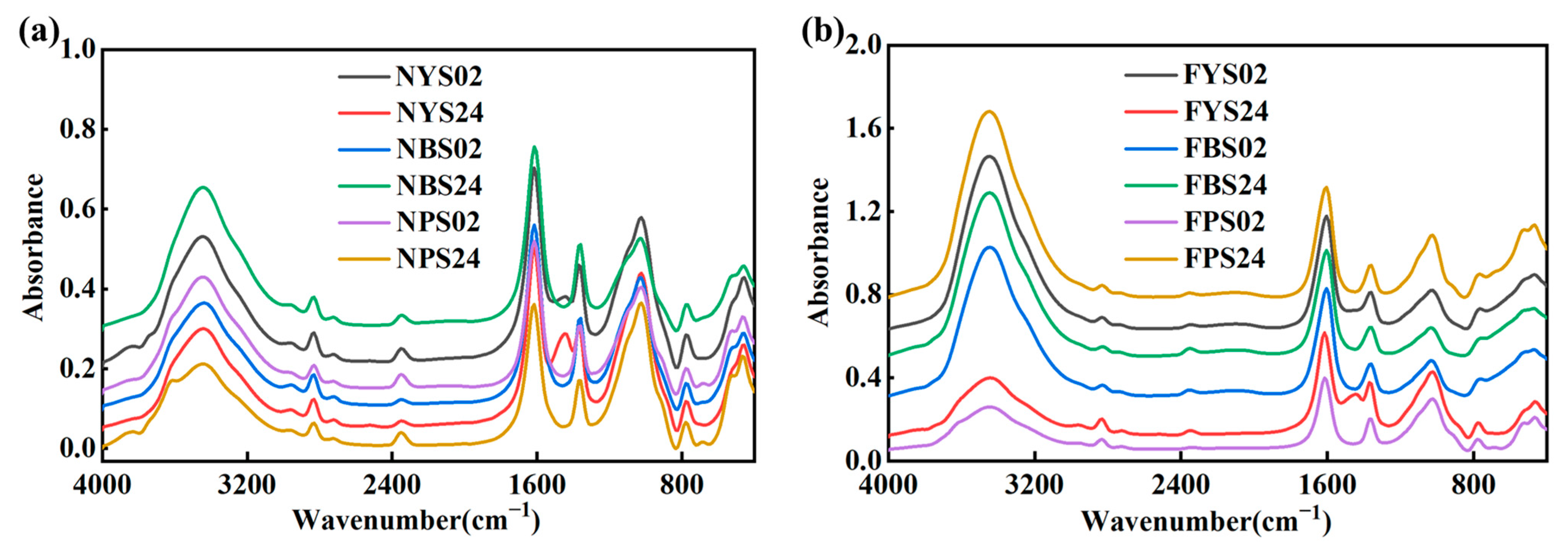
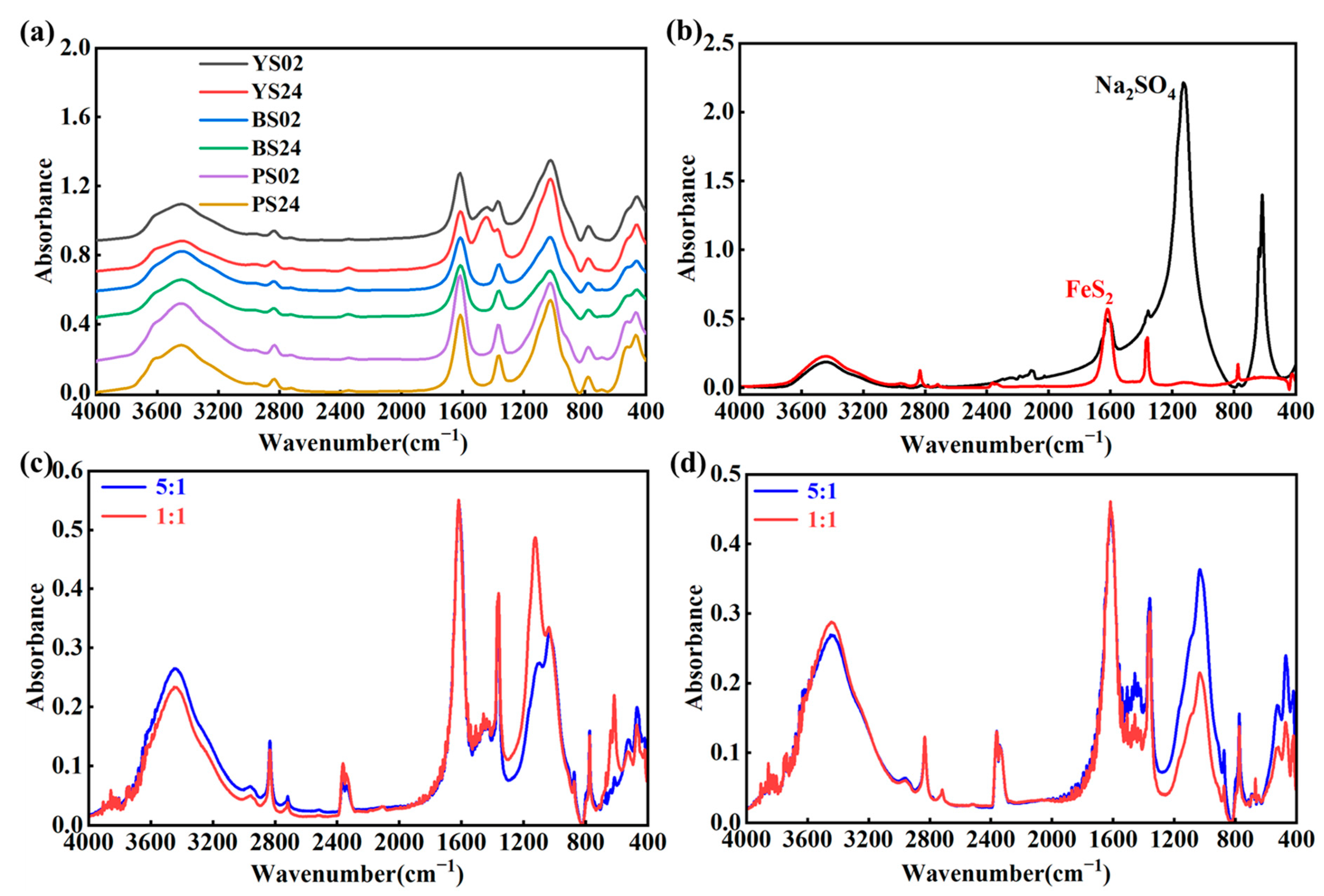
3.1. Spectral Features

Figure 3a illustrates the mid-infrared spectra of the desalinated soil, with hydrogen bonding indicated by a broad absorption band from 3750 to 3250 cm⁻¹ within the single bond region of the spectrum (2500–4000 cm⁻¹). This band confirms the presence of hydrates (H₂O), hydroxyl (-OH), amino compounds, etc. The origin of the bands in the ranges between 790–1240 cm⁻¹ and 1020–1080 cm⁻¹ is attributed to kaolinite and quartz and is usually a fundamental telescopic vibration of the O-Si-O group. Another strong band appears at about 1450 cm⁻¹, indicating the presence of carbonates in the soil. Figure 3b shows the IR of the Na₂SO₄ and FeS₂ pure substances, compared to the standard IR of Na₂SO₄ in the National Institute of Advanced Industrial Science and Technology (NIAIST) database. The peaks of Na₂SO₄ are at 618, 638, 722, 1124, 1366, 1377, 1462, 2096, 2107, 2725, 2853, 2923, and 2963 cm⁻¹. The peaks of FeS₂ are mainly vibrations of the metal–sulfur bond in the 400–700 cm⁻¹ band, and there is a symmetric stretching vibration in the 400–500 cm⁻¹ band, and the relative position between metal and sulfur in the FeS₂ crystals leads to lattice vibrations, which are manifested in the frequency range of 300–400 cm⁻¹.

The Figure 3c,d show the samples mixed with soil and salt at 1:1 (0.1 g:0.1 g) and 1:5 (0.02 g:0.1 g), respectively. The data clearly show that the intensity of the vertical scale increases proportionally with the Na₂SO₄ concentration. which suggests that with the doping of Na₂SO₄, the IR absorption peaks show an enhancement trend. However, in Figure 3d the main features apparent in these plots are the sloping baseline in the mid-infrared (1024 cm⁻¹) and a decrease in intensity of the soil peaks, possibly due to the FeS₂ coating the soil particles. Due to the weakness of these absorption peaks, univariate methods cannot meet the requirements for accurate quantitative analysis. Chemometric methods are the means to quantify sulfate in soil accurately. Therefore, data preprocessing, outlier removal, and the modeling of the above spectra effectively improve the accuracy of determination [39].

3.2. Data Preprocessing

The original spectral data may be affected by the measurement conditions, the working state of the instrument, and the ambient temperature, among other factors. As a result, the original spectrum may contain irrelevant or unwanted information, such as electrical noise, matrix background, stray light, scattering effects, and so on. As a result, preprocessing procedures are critical for eliminating extraneous information and noise from spectral data [40]. Six preprocessing methods were used the SG, baseline, SNV, MSC, F-D, and S-D, respectively, and the statistical results were as follows

Table 2. Modeling results of different pretreatment methods.

Soil Group	Pretreatment Method	Factors	Train		Test
			${\mathit{R}}_{\mathit{c}}^{\mathbf{2}}$	RMSEC	${\mathit{R}}_{\mathbf{p}}^{\mathit{2}}$	RMSEP
NYS02	MSC	8	0.9720	0.0028	0.9306	0.0045
NYS24	F-D	12	0.9909	0.0013	0.9526	0.0033
FYS02	S-D	4	0.9544	0.045	0.9396	0.054
FYS24	S-D	2	0.9378	0.053	0.9320	0.056
NBS02	F-D	6	0.9585	0.0039	0.9409	0.004
NBS24	S-G	4	0.9622	0.0037	0.9252	0.0053
FBS02	S-D	4	0.9604	0.042	0.9402	0.053
FBS24	F-D	5	0.9614	0.041	0.9437	0.052
NPS02	S-D	10	0.9856	0.0021	0.9374	0.0046
NPS24	F-D	9	0.9736	0.0029	0.9111	0.0058
FPS02	S-D	5	0.9768	0.032	0.9673	0.039
FPS24	Baseline	4	0.9558	0.043	0.9432	0.050

. The complete results of all the preprocessing processes are in Supplementary Table S2:

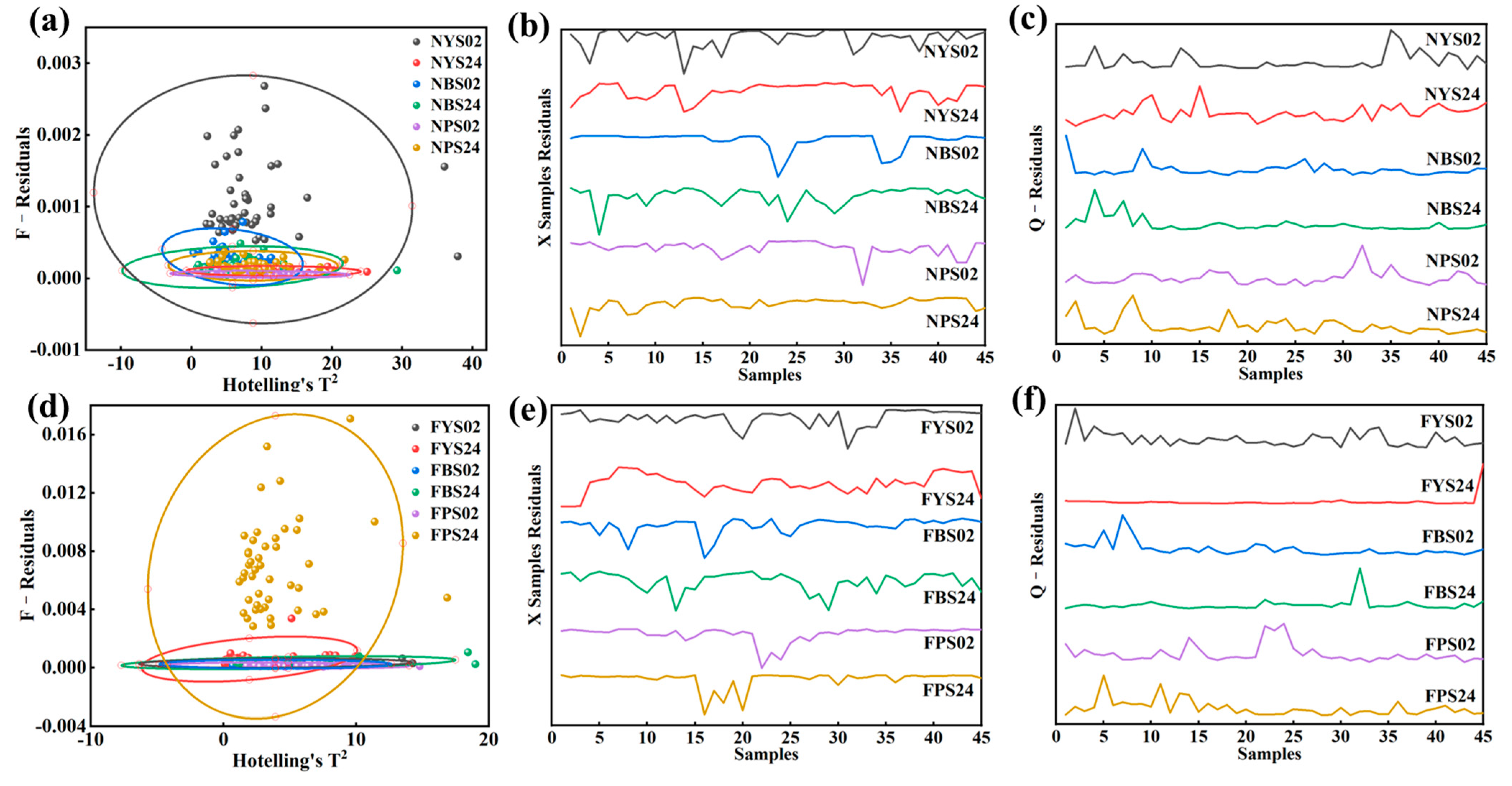
3.3. Outlier Rejection

Due to the different principles of the three methods, T² is based on the Mahalanobis distance from the sample to the overall mean, X-sample variance measures the dispersion of the sample in the model space, and Q residuals measure the distance from the sample to the model. Meanwhile, the distributional assumptions of the statistics are different: the T² statistic follows an F-distribution, the Q-residuals asymptotically follow a weighted chi-square distribution, and the X-sample variance is related to the complexity of the model. This leads to different calculations of critical values. Therefore, the rejection results combining the three methods are displayed in

Table 3. Sample summary of the three outlier culling methods.

Soil Group	Hotelling’s T2 Method	X-Sample ANOVA	Q-Residual Analysis
NYS02	42, 43	13	35
NYS24	15, 38	13, 36	15
NBS02	1	23	1, 9
NBS24	1, 4	4	4, 7
NPS02	32	32	32
NPS24	1	2	2, 8
FYS02	2, 3	31	2
FYS24	4, 45	1, 2, 3	45
FBS02	7	8, 16	7
FBS24	21, 32	13, 29	32
FPS02	38	22, 23, 24	22, 23, 24
FPS24	5, 45	16, 20	5, 11

and Figure 4.

Figure 4a represents Hotelling’s T² method, with samples outside of the 99% confidence interval being anomalous. The outliers were 42 and 43 in NYS02 soils, 15 and 38 in NYS24 soils, 1 in NBS02 soils, 1 and 4 in NBS24 soils, 32 in NPS02 soils, and 1 in NPS24 soils Figure 4b is the X-sample ANOVA; the abscissa represents the number of samples, and the ordinate is the variance. It can be seen that the variance of No. 13 in the NYS02 series soil and the No. 13 and No. 36 variance of the NYS24 series soil is slight, the No. 23 variance of the NBS02 series soil is minor, the No. 4 variance of the NBS24 series soil is minor, the No. 32 variance of the NPS02 series soil is the smallest, and the No. 2 variance of the NPS24 series soil is the smallest. Figure 4c is the Q-residual method; the abscissa represents the number of samples, and the ordinate is the residual. The residuals of No. 35 of the NYS02 series soils are more significant, the residuals of No. 15 of the NYS24 series soils are more significant, the residuals of No. 1 and No. 9 of the NBS02 series soils are more extensive, the residuals of No. 4 and No. 7 of the NBS24 series soils are more extensive, the residuals of No. 32 of the NPS02 series soils are the largest, and the residuals of No. 2 and No. 8 of the NPS24 series soils are more significant. As shown in Figure 4d, the outliers excluded in FYS02 soils were No. 2 and 3, the outliers excluded in FYS24 soils were No. 4 and 45, the outliers excluded in FBS02 soils were No. 7, the outliers eliminated in FBS24 soils were No. 21 and 32, the outlier removed in FPS02 soils was No. 38, and the outliers removed in FPS24 soils were No. 5 and No. 45. As shown in Figure 4e, the variance of No. 31 of the FYS02 series soils is slight, and it can be seen that the overall variance in the FYS24 series soils is slight. Still, the variances in No. 1, 2, and 3 are minimal, the variance in No. 8 and No. 16 of the FBS02 series soils is minor, the variance in No. 13 and No. 29 of the FBS24 series soils is minor, the variance in No. 22, 23, and 24 is the smallest in the FPS02 series soils, and the variance in No. 16 and No. 20 of the FPS24 series soils is smaller than that of the other samples. As shown in Figure 4f, the residuals of No. 2 of FYS02 series soil are more significant, the residuals of No. 45 of FYS24 series soil are the largest, the residuals of No. 7 of FBS02 series soil are more extensive, the residuals of No. 32 of FBS24 series soil are the largest, the residuals of No. 22, 23, and 24 of FPS02 series soil are the largest, and the residuals of No. 5 and No. 11 of FPS24 series soil are more significant. All outliers were removed, after which the remaining samples were modeled and analyzed according to the preprocessing method in Section 3.2.

3.4. Identification of Key Wavelengths

Selecting the spectrum characteristic bands to construct the model may considerably limit the interference of redundant information, consequently enhancing the prediction accuracy and stability of the model [41]. We conducted a correlation analysis between full-spectrum data and soil sulfate content, discovering that the wavelengths highlighted in red in Figure 5 exhibited higher correlation coefficients with sulfate content. These wavelengths were found to be more sensitive to variations in sulfate content. The red coverage area was selected as the feature band for predictive analysis, as shown in

Table 4. Characteristic wavelengths for each sample set and screening modeling bands.

Soil Group	Important Wavelengths (cm−1)	Model Wavelengths (cm−1)
NYS02	622 cm−1, 1069–1258 cm−1, 1537 cm−1, 1693 cm−1, 3735 cm−1	1069–1258 cm−1
NYS24	589 cm−1, 1046 cm−1, 1102 cm−1, 1615 cm−1, 3433 cm−1	1002–1124 cm−1
NBS02	600 cm−1, 656 cm−1, 1102 cm−1, 1180 cm−1	901–1281 cm−1
NBS24	622 cm−1, 1124 cm−1,1381 cm−1, 1426 cm−1	991–1292 cm−1
NPS02	578 cm−1, 622 cm−1, 689 cm−1, 745 cm−1, 1381 cm−1, 2381 cm−1, 2865 cm−1	567–734 cm−1
NPS24	600 cm−1, 656 cm−1, 2351 cm−1, 2356 cm−1	511–734 cm−1
FYS02	834 cm−1, 1024 cm−1	957–1069 cm−1
FYS24	455 cm−1, 834 cm−1, 946 cm−1, 1024 cm−1, 1359 cm−1, 1437 cm−1	946–1069 cm−1
FBS02	790 cm−1, 834 cm−1, 1046 cm−1, 1080 cm−1	790–1091 cm−1
FBS24	801 cm−1, 857 cm−1, 1002 cm−1	779–1057 cm−1
FPS02	834 cm−1, 890 cm−1, 979 cm−1, 2351 cm−1, 2396 cm−1	790–1091 cm−1
FPS24	455 cm−1, 890–1247 cm−1, 1593 cm−1	890–1247 cm−1

.

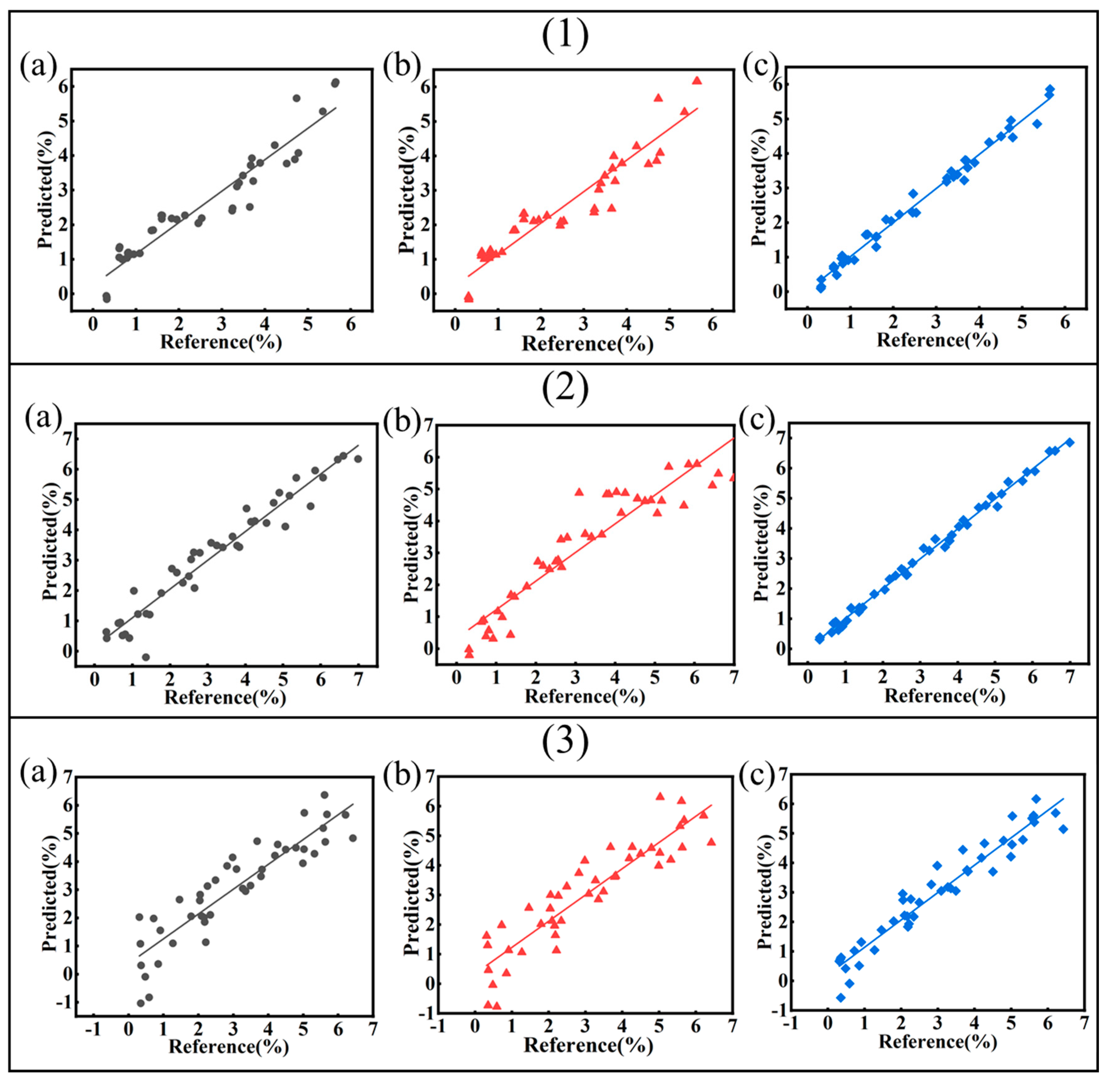
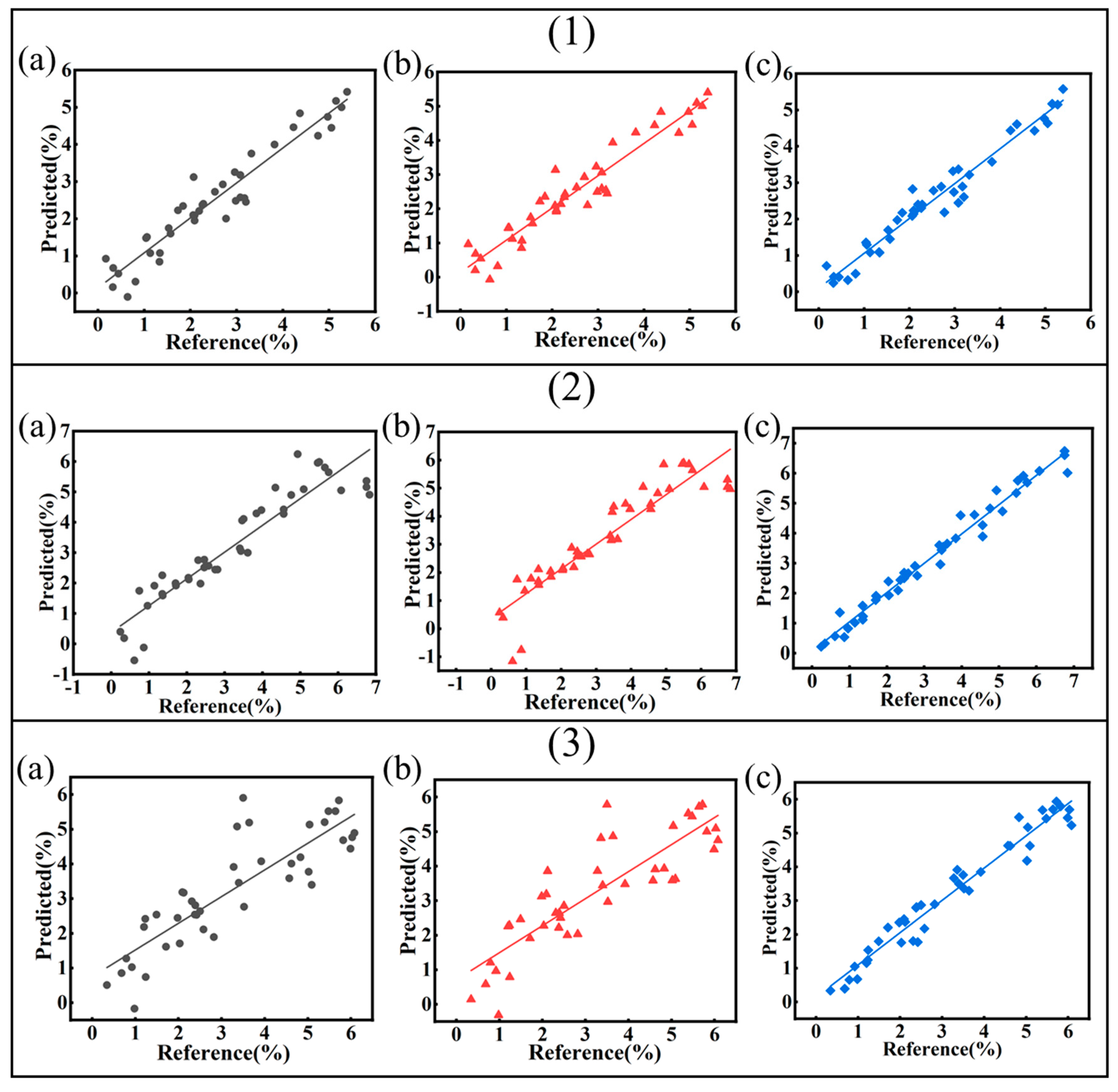
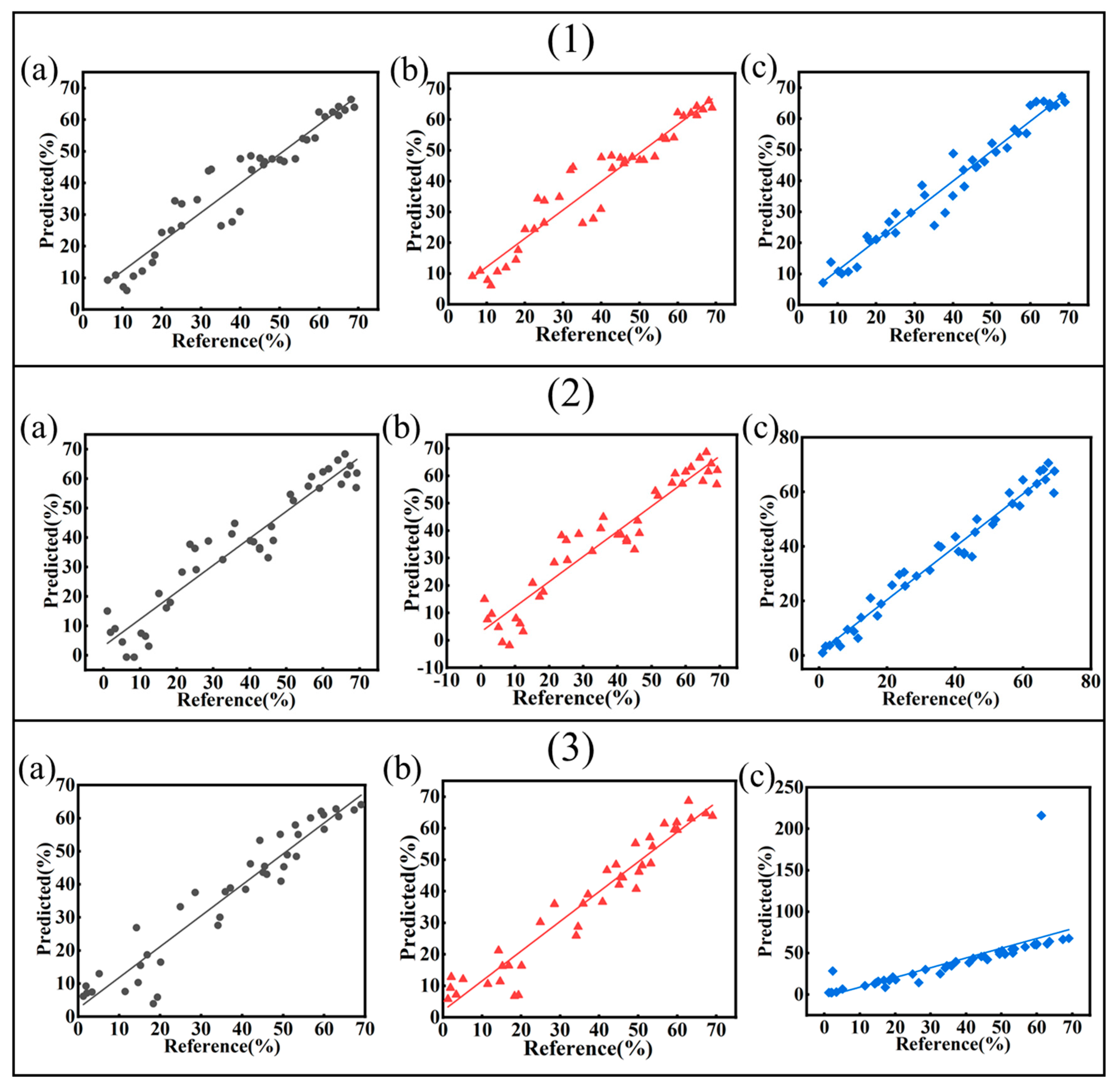
3.5. Establishment and Validation of Regression Models

The performance and index results and predictions of mid-infrared spectroscopy evaluate the model’s performance in the mid-infrared spectral range. Considering the importance of parameters such as RPD and RMSE in spectral data analysis, this study focuses on evaluating these indicators. In this scenario, points above the fitted line in each figure represent spectrum-predicted values higher than those seen in the laboratory. In contrast, points below the fitted line represent values predicted by the spectrum lower than those in the laboratory.

3.5.1. Regression Modeling of Soluble Salts

As shown in

Table 5. Comparison of the results of the training and prediction sets of the readily soluble salt regression model.

Soil Group	Regression Model	Factors	Training		Validation
			${\mathit{R}}_{\mathit{c}}^{\mathbf{2}}$	RMSEC	${\mathit{R}}_{\mathbf{p}}^{\mathit{2}}$	RMSEP	RPD	RPIQ
NYS02	MSC-PLSR	3	0.9164	0.0046	0.9103	0.0050	3.52	5.52
	MSC-PCR	3	0.9160	0.0047	0.9108	0.0051	3.19	5.42
	MSC-MLR	-	0.9856	0.0026	0.9832	0.0020	8.44	14.32
NYS24	FD-PLSR	7	0.9483	0.0033	0.9231	0.0042	3.53	4.46
	FD-PCR	7	0.9471	0.0034	0.9209	0.0042	3.51	4.43
	FD-MLR	-	0.9583	0.0036	0.9535	0.0030	4.96	6.26
NBS02	FD-PLSR	6	0.9649	0.0035	0.9440	0.0047	4.03	7.05
	FD-PCR	4	0.8997	0.0060	0.8777	0.0067	2.86	5.01
	FD-MLR	-	0.9941	0.0038	0.9396	0.0045	13.24	23.17
NBS24	SG-PLSR	3	0.9013	0.0059	0.8770	0.0068	2.79	4.46
	SG-PCR	4	0.8916	0.0062	0.8605	0.0072	2.64	4.21
	SG-MLR	-	0.9766	0.0051	0.9192	0.0051	6.62	10.59
NPS02	SD-PLSR	9	0.8954	0.0058	0.8233	0.0078	2.33	3.84
	SD-PCR	9	0.8974	0.0058	0.8277	0.0076	2.41	3.97
	SD-MLR	-	0.9280	0.0060	0.9274	0.0048	3.77	6.20
NPS24	FD-PLSR	3	0.7923	0.0079	0.7438	0.0090	1.94	3.34
	FD-PCR	5	0.8157	0.0074	0.7390	0.0089	1.96	3.38
	FD-MLR	-	0.9555	0.0053	0.9388	0.0041	4.80	8.28

, according to the study, the optimal predictive models for YS, BS, and PS soils containing sodium sulfate at a 0–20 cm depth were MSC-MLR, FD-MLR, and SD-MLR, respectively. For the 0–20 cm soil in the SO₄²⁻ detection, the average R_P² of the MLR model was 0.9501, the average RMSEP was 0.37%, and the average RPD was 8.48. The average RPIQ was 14.56, indicating that the model proposed in this study can make reliable predictions when the SO₄²⁻ content is higher than 0.37%. We show the effect of model training and fit it with a scatterplot, as shown in Figure 6.

The MLR model provided the best predictive performance for YS, BS, and PS soil groups mixed with sodium sulfate at the 20–40 cm depth. For the detection of SO₄²⁻ in soils from 20 to 40 cm, the average R_P² of the MLR model was 0.9371, the average RMSEP was 0.41%, the average RPD was 5.32, and the average RPIQ was 8.38, indicating that the model proposed in this study can make reliable predictions when the SO₄²⁻ content is higher than 0.41%. We show the effect of model training and fit it with a scatterplot, as shown in Figure 7.

3.5.2. Regression Modeling of Sulfide

As summarized in

Table 6. Comparison of training and prediction set results for sulfide regression models.

Soil Group	Regression Model	Factors	Training		Validation
			${\mathit{R}}_{\mathit{c}}^{\mathbf{2}}$	RMSEC	${\mathit{R}}_{\mathbf{p}}^{\mathit{2}}$	RMSEP	RPD	RPIQ
FYS02	SD-PLSR	3	0.9009	0.065	0.8865	0.072	2.89	4.98
	SD-PCR	3	0.8979	0.066	0.8765	0.071	2.93	5.04
	SD-MLR	-	0.9304	0.066	0.9275	0.053	3.84	6.61
FYS24	SD-PLSR	1	0.9277	0.050	0.9260	0.053	3.61	6.30
	SD-PCR	1	0.9277	0.050	0.9262	0.052	3.63	6.32
	SD-MLR	-	0.9620	0.044	0.3825	0.14	5.20	9.06
FBS02	SD-PLSR	6	0.9365	0.053	0.8865	0.072	2.97	5.10
	SD-PCR	7	0.9046	0.065	0.8745	0.075	2.86	4.90
	SD-MLR	-	0.9809	0.052	0.9540	0.044	7.32	12.55
FBS24	FD-PLSR	2	0.9204	0.061	0.9137	0.065	3.37	6.18
	FD-PCR	2	0.9199	0.062	0.9097	0.066	3.33	6.11
	FD-MLR	-	0.9712	0.063	0.9590	0.042	5.97	10.94
FPS02	FD-PLSR	2	0.9573	0.044	0.9503	0.049	4.44	7.97
	FD-PCR	3	0.9577	0.044	0.9508	0.048	4.52	8.12
	FD-MLR	-	0.9949	0.028	0.9848	0.025	14.20	25.48
FPS24	Baseline-PLSR	5	0.9445	0.048	0.9206	0.058	3.51	6.03
	Baseline-PCR	6	0.9517	0.044	0.9363	0.053	3.88	6.67
	Baseline-MLR	-	0.9939	0.040	0.5217	0.23	0.88	1.52

, for the YS, BS, and PS soil groups with iron disulfide added at 0–20 cm of depth, the MLR model demonstrated the best predictive performance. In the case of detecting FeS₂ in soil samples from a depth of 0–20 cm, the MLR model achieved an average R_P² of 0.9554, an average RMSE_P of 4.07%, an average RPD of 8.45, and an average RPIQ of 14.88. These results indicate that the proposed model can provide reliable predictions when the FeS₂ content in the soil exceeds 4.07%. A scatterplot illustrating these results is presented in Figure 8.

The PCR model performed best for the YS soils of 20–40 cm doped with iron disulfide, and the MLR model best performed for the BS and PS soil models. For the detection of FeS₂ in soils from 20 to 40 cm, the average R_P² of the MLR model was 0.9405, the average RMSEP was 4.9%, the average RPD was 4.49, and the average RPIQ was 7.98, indicating that the model proposed in this study can make reliable predictions when the FeS₂ content in soil is higher than 4.9%. A scatterplot illustrating these results is presented in Figure 9.

4. Discussion

4.1. Interpretation of Mid-Infrared Spectra

The mid-infrared sulfate spectra are predominantly influenced by the vibrations of the S-O bond in SO₄²⁻, occasionally disrupted by O-H, H₂O, and CO₃²⁻. The complexation of cations in solid sulfates results in the distortion of the sulfate polyhedral structure and a departure from Td symmetry, leading to alterations in the spectral characteristics, including band splitting. The S-O distance exhibits minor variations among different minerals, with an average measurement of 1.473 Å. The infrared vibrational characteristics of sulfates generally manifest throughout the ranges of around 1050–1250 cm⁻¹ (v₃), around 1000 cm⁻¹ (v₁), approximately 500–700 cm⁻¹ (v₄), and roughly 400–500 cm⁻¹ (v₂). However, the lattice vibrations predominantly reside in the region below 550 cm⁻¹ [17]. In magnesium alum hydrate, the v₃ band for sulfate is situated at 1256 and 1183 cm⁻¹, accompanied by a weak third band at about 1213 cm⁻¹; the v₁ band is found at 1045 cm⁻¹; the v₄ band appears at 669, 641, and approximately 610 cm⁻¹; and the v₂ band is placed at 458 cm⁻¹. The sulfate tetrahedra in the magnesium alum exhibit C₂ symmetry, with the v₂ band typically being faint or challenging to detect [42].

Plagioclase is also a monohydrate sulfate and is considered to be the end element in the solid solution series with sodium orthosilicate. The spectrum of this boromagnesian ferrite is very similar to that of sodium–magnesian alum; however, the spectral signature of boromagnesian ferrite is shifted by about 20–100 wave numbers to longer wavelengths. The SO₄²⁻ internal vibrational bands are distinct in the spectra, consisting of three v₃ bands at 1226, 1195, and 1149 cm⁻¹. The v₁ band occurs as a minor feature at 1018 cm⁻¹. v₄ vibrations produce the features at 626, 606, and 554 cm⁻¹. The strange emission signal at 846 cm⁻¹ comes from water vibrations [43], and the sharp feature near 669 cm⁻¹ is caused by CO₂ in the sample chamber, not the mineral sample itself. Distortions of the SO₄⁻ tetrahedra cause several absorption patterns connected to sulfate. The number of spectral bands supports the C2-site symmetry of SO₄²⁻ in a square zeolite, a mineral from the diatomaceous earth group.

4.2. Comparison of Chemometrics Methods with Deep Learning Methods

This study employed three classical chemometric methods (PLSR, PCR, and MLR) rather than deep learning approaches for spectral data analysis. Although deep learning methods have gained widespread applications in spectral analysis in recent years, chemometric methods offer multiple advantages for this study’s specific objectives and available data conditions. First, deep learning methods typically require large training sample sizes to obtain reliable models, whereas our relatively limited sample quantity makes chemometric methods more effective for utilizing existing data. Chemometric methods are particularly suited for handling high-dimensional, multicollinear spectral data and can establish robust models with smaller sample sets.

Second, chemometric methods provide highly interpretable model structures. Unlike the ‘black box’ nature of deep learning, these methods allow us to identify and interpret spectral regions that significantly contribute to prediction results, which is crucial for understanding the relationships between sulfates, sulfides, and spectral features. Additionally, chemometric methods have relatively low computational resource requirements, making model training and validation processes more efficient and especially suitable for laboratory applications. While deep learning may perform better when processing complex, non-linear relationships in large datasets, chemometric methods are more appropriate considering this study’s sample size, specific requirements, and the importance of result interpretation.

4.3. Excellent Performance of MLR

The MLR model showed significant advantages in predicting the content of sodium sulfate and iron disulfide in soil, which was mainly attributed to its comprehensive retention and utilization of spectral information. Unlike dimensionality reduction techniques such as PLSR and PCR, MLR directly utilizes the raw or preprocessed spectral data to build the prediction model, avoiding the loss of information that may occur during the dimensionality reduction process. Especially for sodium sulfate and iron disulfide in this study, these compounds have specific spectral fingerprint features in the mid-infrared region. MLR can fully capture these feature peaks’ complex interactions and subtle changes. PLSR and PCR by principal component or latent variable downscaling, while able to deal with the problem of multicollinearity, may lose the key spectral information of sulfate and sulfide. Our study suggests that the intact retention of spectral information is more important than treating multicollinearity problems for the soil samples and target compounds in this study. This finding challenges the generally accepted theory of PLSR dominance in spectral analysis and highlights the importance of choosing the appropriate modeling method in a particular application context. In particular, when combined with appropriate preprocessing methods such as derivative transformations, MLR effectively deals with baseline drift and background interferences while preserving the complete spectral information to achieve the best prediction performance.

5. Conclusions

In this study, we successfully predicted sulfate and sulfide content in soil using mid-infrared spectroscopy combined with multiple preprocessing methods and chemometric modeling. The results demonstrated that different soil types responded variably to preprocessing techniques, highlighting the importance of preprocessing method selection for optimizing model performance. While conventional PLSR and PCR performed well with certain soil types, the MLR model consistently demonstrated superior predictive accuracy in most scenarios. For instance, when analyzing iron disulfide in 0–20 cm southwestern subtropical soils, the MLR model coupled with first-derivative preprocessing achieved optimal performance. This was evidenced by an R²p of 0.9848, an RMSEP of 0.025, an RPD of 14.20, and an RPIQ of 25.48. The enhanced results likely stem from MLR’s retention of more comprehensive spectral information, minimizing the data loss inherent in dimensionality reduction techniques like PLSR and PCR. The soil matrix is highly complex, with overlapping spectral responses from organic matter and inorganic minerals interfering. Organic matter produces characteristic mid-infrared absorption peaks through its functional groups, often overlapping with inorganic mineral signals. Additionally, kaolinite and montmorillonite exhibit distinct absorption features in the mid-infrared region due to their unique silica–oxygen tetrahedral and aluminum–oxygen octahedral structures. Soil type and physicochemical properties significantly influence spectral response characteristics, necessitating region-specific model development through tailored preprocessing methods and modeling strategies. In some datasets, significant differences were found between the MLR models. This highlights the importance of prioritizing model robustness and generalization capability in practical applications rather than relying solely on individual performance metrics. Compared to traditional wet chemistry methods, this approach offers significant speed, cost-effectiveness, and non-destructiveness advantages, presenting a promising technical solution for soil nutrient management and environmental monitoring. Future research should incorporate larger sample sizes, encompassing broader soil varieties to validate and optimize the model further, thereby enhancing its applicability and robustness.

References

1. Radha, B.; Sunitha, N.C.; Sah, R.P.; Tp, M.A.; Krishna, G.; Umesh, D.K.; Thomas, S.; Anilkumar, C.; Upadhyay, S.; Kumar, A. Physiological and molecular implications of multiple abiotic stresses on yield and quality of rice. Front. Plant Sci. 2023, 13, 996514. [Google Scholar] [CrossRef] [PubMed]
2. Hopmans, J.W.; Qureshi, A.; Kisekka, I.; Munns, R.; Grattan, S.; Rengasamy, P.; Ben-Gal, A.; Assouline, S.; Javaux, M.; Minhas, P. Critical knowledge gaps and research priorities in global soil salinity. Adv. Agron. 2021, 169, 1–191. [Google Scholar]
3. Santhanam, M.; Cohen, M.D.; Olek, J. Sulfate attack research—Whither now? Cem. Concr. Res. 2001, 31, 845–851. [Google Scholar] [CrossRef]
4. Ma, Z.; Zhou, L.; Yu, W.; Yang, Y.; Teng, H.; Shi, Z. Improving TMPA 3B43 V7 data sets using land-surface characteristics and ground observations on the Qinghai–Tibet Plateau. IEEE Geosci. Remote Sens. Lett. 2018, 15, 178–182. [Google Scholar] [CrossRef]
5. Wang, J.; Ding, J.; Yu, D.; Ma, X.; Zhang, Z.; Ge, X.; Teng, D.; Li, X.; Liang, J.; Lizaga, I. Capability of Sentinel-2 MSI data for monitoring and mapping of soil salinity in dry and wet seasons in the Ebinur Lake region, Xinjiang, China. Geoderma 2019, 353, 172–187. [Google Scholar] [CrossRef]
6. Wang, N.; Xue, J.; Peng, J.; Biswas, A.; He, Y.; Shi, Z. Integrating remote sensing and landscape characteristics to estimate soil salinity using machine learning methods: A case study from Southern Xinjiang, China. Remote Sens. 2020, 12, 4118. [Google Scholar] [CrossRef]
7. Dent, D.; Pons, L. A world perspective on acid sulphate soils. Geoderma 1995, 67, 263–276. [Google Scholar] [CrossRef]
8. Fanning, D.S.; Rabenhorst, M.C.; Fitzpatrick, R.W. Historical developments in the understanding of acid sulfate soils. Geoderma 2017, 308, 191–206. [Google Scholar] [CrossRef]
9. Nelson, M.D.; Riitters, K.H.; Coulston, J.W.; Domke, G.M.; Greenfield, E.J.; Langner, L.L.; Nowak, D.J.; O’Dea, C.B.; Oswalt, S.N.; Reeves, M.C.; et al. Defining the United States land base: A technical document supporting the USDA Forest Service 2020 RPA assessment. Gen. Tech. Rep. NRS-191 2020, 191, 1–70. [Google Scholar]
10. Douglas, R.; Nawar, S.; Alamar, M.C.; Coulon, F.; Mouazen, A.M. Almost 25 years of chromatographic and spectroscopic analytical method development for petroleum hydrocarbons analysis in soil and sediment: State-of-the-art, progress and trends. Crit. Rev. Environ. Sci. Technol. 2017, 47, 1497–1527. [Google Scholar] [CrossRef]
11. Siesler, H.W.; Ozaki, Y.; Kawata, S.; Heise, H.M. Near-Infrared Spectroscopy: Principles, Instruments, Applications; John Wiley & Sons: Hoboken, NJ, USA, 2008. [Google Scholar]
12. Barra, I.; Haefele, S.M.; Sakrabani, R.; Kebede, F. Soil spectroscopy with the use of chemometrics, machine learning and pre-processing techniques in soil diagnosis: Recent advances—A review. TrAC Trends Anal. Chem. 2021, 135, 116166. [Google Scholar] [CrossRef]
13. Helfenstein, A.; Baumann, P.; Viscarra Rossel, R.; Gubler, A.; Oechslin, S.; Six, J. Quantifying soil carbon in temperate peatlands using a mid-IR soil spectral library. Soil 2021, 7, 193–215. [Google Scholar] [CrossRef]
14. Xing, Z.; Du, C.; Tian, K.; Ma, F.; Shen, Y.; Zhou, J. Application of FTIR-PAS and Raman spectroscopies for the determination of organic matter in farmland soils. Talanta 2016, 158, 262–269. [Google Scholar] [CrossRef] [PubMed]
15. Yan, C.; Zhang, T.; Sun, Y.; Tang, H.; Li, H. A hybrid variable selection method based on wavelet transform and mean impact value for calorific value determination of coal using laser-induced breakdown spectroscopy and kernel extreme learning machine. Spectrochim. Acta Part B At. Spectrosc. 2019, 154, 75–81. [Google Scholar] [CrossRef]
16. Zhang, H.; Fu, X.; Zhang, Y.; Qi, Z.; Zhang, H.; Xu, Z. Mapping multi-depth soil salinity using remote sensing-enabled machine learning in the yellow river delta, China. Remote Sens. 2023, 15, 5640. [Google Scholar] [CrossRef]
17. Lotfollahi, L.; Delavar, M.A.; Biswas, A.; Fatehi, S.; Scholten, T. Spectral prediction of soil salinity and alkalinity indicators using visible, near-, and mid-infrared spectroscopy. J. Environ. Manag. 2023, 345, 118854. [Google Scholar] [CrossRef] [PubMed]
18. Yin, J.; Shi, Z.; Li, B.; Sun, F.; Miao, T.; Shi, Z.; Chen, S.; Yang, M.; Ji, W. Prediction of soil properties in a field in typical black soil areas using in situ MIR spectra and its comparison with vis-NIR spectra. Remote Sens. 2023, 15, 2053. [Google Scholar] [CrossRef]
19. Canero, F.M.; Rodriguez-Galiano, V.; Aragones, D. Machine Learning and Feature Selection for soil spectroscopy. An evaluation of Random Forest wrappers to predict soil organic matter, clay, and carbonates. Heliyon 2024, 10, e30228. [Google Scholar] [CrossRef]
20. Zhan, D.; Liu, Y.; Yang, W.; Lu, M.; Song, Y. Spatial variability of soil salinity in coastal saline-alkali farmlands: A novel approach integrating a stacked model with the reconstructed in-situ hyperspectral feature. Comput. Electron. Agric. 2025, 235, 110376. [Google Scholar] [CrossRef]
21. dos Santos, E.P.; Moreira, M.C.; Fernandes-Filho, E.I.; Demattê, J.A.M.; Santos, U.J.D.; Moura-Bueno, J.M.; Cruz, R.R.P.; da Silva, D.D.; de Sá Barreto Sampaio, E.V. Integrating satellite radar vegetation indices and environmental descriptors with visible-infrared soil spectroscopy improved organic carbon prediction in soils of semi-arid Brazil. Geoderma 2025, 457, 117288. [Google Scholar] [CrossRef]
22. Xia, Y.; Cheng, X.; Hu, X. Soil organic matter content prediction in tobacco fields based on hyperspectral remote sensing and generative adversarial network data augmentation. Comput. Electron. Agric. 2025, 233, 110164. [Google Scholar] [CrossRef]
23. Savitzky, A.; Golay, M.J. Smoothing and differentiation of data by simplified least squares procedures. Anal. Chem. 1964, 36, 1627–1639. [Google Scholar] [CrossRef]
24. Lieber, C.A.; Mahadevan-Jansen, A. Automated method for subtraction of fluorescence from biological Raman spectra. Appl. Spectrosc. 2003, 57, 1363–1367. [Google Scholar] [CrossRef]
25. Barnes, R.; Dhanoa, M.S.; Lister, S.J. Standard normal variate transformation and de-trending of near-infrared diffuse reflectance spectra. Appl. Spectrosc. 1989, 43, 772–777. [Google Scholar] [CrossRef]
26. Geladi, P.; MacDougall, D.; Martens, H. Linearization and scatter-correction for near-infrared reflectance spectra of meat. Appl. Spectrosc. 1985, 39, 491–500. [Google Scholar] [CrossRef]
27. Rinnan, Å.; Van Den Berg, F.; Engelsen, S.B. Review of the most common pre-processing techniques for near-infrared spectra. TrAC Trends Anal. Chem. 2009, 28, 1201–1222. [Google Scholar] [CrossRef]
28. Mehmood, T. Hotelling T2 based variable selection in partial least squares regression. Chemom. Intell. Lab. Syst. 2016, 154, 23–28. [Google Scholar] [CrossRef]
29. Connelly, L.M. Introduction to Analysis of Variance (ANOVA). Medsurg Nursing. 2021, 30, 3. [Google Scholar] [CrossRef]
30. Chen, J. A residual-based approach to validate Q-matrix specifications. Appl. Psychol. Meas. 2017, 41, 277–293. [Google Scholar] [CrossRef]
31. Ma, Y.; Roudier, P.; Kumar, K.; Palmada, T.; Grealish, G.; Carrick, S.; Lilburne, L.; Triantafilis, J. A soil spectral library of New Zealand. Geoderma Reg. 2023, 35, e00726. [Google Scholar] [CrossRef]
32. Mevik, B.H.; Wehrens, R. The pls package: Principal component and partial least squares regression in R. J. Stat. Softw. 2007, 18, 1–23. [Google Scholar] [CrossRef]
33. Soriano-Disla, J.M.; Janik, L.J.; Forrester, S.T.; Grocke, S.F.; Fitzpatrick, R.W.; McLaughlin, M.J. The use of mid-infrared diffuse reflectance spectroscopy for acid sulfate soil analysis. Sci. Total Environ. 2019, 646, 1489–1502. [Google Scholar] [CrossRef] [PubMed]
34. Lawrence, I.; Lin, K. A concordance correlation coefficient to evaluate reproducibility. Biometrics 1989, 45, 255–268. [Google Scholar]
35. Williams, P.; Thompson, B. BY NEAR INFRARED REFLECTANCE SPECTROSCOPY (NRS). Cereal Chem. 1978, 55, 1014–1037. [Google Scholar]
36. Bellon-Maurel, V.; Fernandez-Ahumada, E.; Palagos, B.; Roger, J.-M.; McBratney, A. Critical review of chemometric indicators commonly used for assessing the quality of the prediction of soil attributes by NIR spectroscopy. TrAC Trends Anal. Chem. 2010, 29, 1073–1081. [Google Scholar] [CrossRef]
37. Vohland, M.; Besold, J.; Hill, J.; Fründ, H.-C. Comparing different multivariate calibration methods for the determination of soil organic carbon pools with visible to near infrared spectroscopy. Geoderma 2011, 166, 198–205. [Google Scholar] [CrossRef]
38. Rossel, R.V.; Behrens, T.; Ben-Dor, E.; Brown, D.; Demattê, J.A.M.; Shepherd, K.D.; Shi, Z.; Stenberg, B.; Stevens, A.; Adamchuk, V. A global spectral library to characterize the world’s soil. Earth-Sci. Rev. 2016, 155, 198–230. [Google Scholar] [CrossRef]
39. Li, X.; Fan, P.; Qiu, H.; Liu, Y. Optimizing soil carbon content prediction performance by multi-band feature fusion based on visible near-infrared spectroscopy. J. Soils Sediments 2024, 24, 1333–1347. [Google Scholar] [CrossRef]
40. Engel, J.; Gerretzen, J.; Szymańska, E.; Jansen, J.J.; Downey, G.; Blanchet, L.; Buydens, L.M. Breaking with trends in pre-processing? TrAC Trends Anal. Chem. 2013, 50, 96–106. [Google Scholar] [CrossRef]
41. Xiaobo, Z.; Jiewen, Z.; Povey, M.J.; Holmes, M.; Hanpin, M. Variables selection methods in near-infrared spectroscopy. Anal. Chim. Acta 2010, 667, 14–32. [Google Scholar] [CrossRef]
42. Hezel, A.T.; Ross, S. Forbidden transitions in the infra-red spectra of tetrahedral anions—III. Spectra-structure correlations in perchlorates, sulphates and phosphates of the formula MXO4. Spectrochim. Acta 1966, 22, 1949–1961. [Google Scholar] [CrossRef]
43. Grodzicki, A.; Piszczek, P. A new interpretation of abnormal shift of water molecules’ bending vibration frequencies in kieserite family monohydrates. J. Mol. Struct. 1998, 443, 141–147. [Google Scholar] [CrossRef]
Figure 1. The study area: (a) location of the study area; (bd) soil profiles.
Chemosensors 13 00173 g001
Figure 2. (a) Average spectrum of soil mixture with added sodium sulfate. (b) Average spectra of mixed soils with added iron disulfide.
Chemosensors 13 00173 g002
Figure 3. (a) Infrared spectra of desalinated soil after water washing. (b) Spectral dataset plots of the mid-infrared spectra of Na2SO4 and FeS2. (c) Mid-infrared spectra of soil with spiking with Na2SO4; 1:1 and 5:1 mixed observation of SO42− characteristic peaks. (d) Mid-infrared spectra of soil with spiking with FeS2; 1:1 and 5:1 mixed observation of SO42− characteristic peaks.
Chemosensors 13 00173 g003
Figure 4. (a) NYS series soils, Hotelling’s T2 method, (b) NYS series soils, X-sample ANOVA, (c) NYS series soils, Q-residual analysis, (d) FYS series soils, Hotelling’s T2, (e) FYS series soils, X-sample ANOVA, (f) FYS series soils, Q-residual analysis.
Chemosensors 13 00173 g004
Figure 5. Plot of weighted regression coefficients. (a) YS soil 0–20 cm and 20–40 cm mixed with sodium sulfate, (b) YS soil 0–20 cm and 20–40 cm mixed with iron disulfide, (c) BS soil 0–20 cm and 20–40 cm mixed with sodium sulphate, (d) BS soil 0–20 cm and 20–40 cm mixed with iron disulfide, (e) PS soil 0–20 cm and 20–40 cm mixed with sodium sulphate, (f) PS soil 0–20 cm and 20–40 cm mixed with iron disulfide.
Chemosensors 13 00173 g005
Figure 6. Validation plot of predicted sulfate spectra of 0–20 cm soil mixed with sodium sulfate against laboratory reference values. (1) YS (a) PLSR, (b) PCR, and (c) MLR; (2) BS (a) PLSR, (b) PCR, and (c) MLR; (3) PS (a) PLSR, (b) PCR, and (c) MLR.
Chemosensors 13 00173 g006
Figure 7. Validation plot of predicted sulfate spectra of 20–40 cm soil mixed with sodium sulfate against laboratory reference values. (1) YS: (a) PLSR, (b) PCR, and (c)MLR; (2) BS: (a) PLSR, (b) PCR, and (c) MLR; (3) PS: (a) PLSR, (b) PCR, and (c) MLR.
Chemosensors 13 00173 g007
Figure 8. Validation plot comparing predicted sulfide spectral signatures in 0–20 cm soil samples amended with FeS2 against laboratory reference measurements. (1) YS: (a) PLSR, (b) PCR, and (c) MLR; (2) BS: (a) PLSR, (b) PCR, and (c) MLR; (3) PS: (a) PLSR, (b) PCR, and (c) MLR.
Chemosensors 13 00173 g008
Figure 9. Validation plot comparing predicted sulfide spectral signatures in 20–40 cm soil samples amended with FeS2 against laboratory reference measurements. (1) YS: (a) PLSR, (b) PCR, and (c) MLR; (2) BS: (a) PLSR, (b) PCR, and (c) MLR; (3) PS: (a) PLSR, (b) PCR, and (c) MLR.
Chemosensors 13 00173 g009