Article

Fusion Recalibration Method for Addressing Multiplicative and Additive Effects and Peak Shifts in Analytical Chemistry

1
College of Computer and Control Engineering, Northeast Forestry University, Harbin 150040, China
2
College of Mechanical and Electrical Engineering, Northeast Forestry University, Harbin 150040, China
*
Author to whom correspondence should be addressed.
These authors contributed equally to this work.
Current address: College of Computer Science and Artificial Intelligence, Changzhou University, Changzhou 213164, China.
Chemosensors 2023, 11(9), 472; https://doi.org/10.3390/chemosensors11090472
Submission received: 17 July 2023 / Revised: 12 August 2023 / Accepted: 16 August 2023 / Published: 23 August 2023

Abstract

:
Analytical chemistry relies on the qualitative and quantitative analysis of multivariate data obtained from various measurement techniques. However, artifacts such as missing data, noise, multiplicative and additive effects, and peak shifts can adversely affect the accuracy of chemical measurements. To ensure the validity and accuracy of results, it is crucial to preprocess the data and correct for these artifacts. This paper proposes a fusion recalibration algorithm, called Spectral Offset Recalibration (SOR), that combines the Extended Multiplicative Signal Correction (EMSC) and Correlation-Optimized Warping (COW) algorithms to address both multiplicative and additive effects and peak shifts. The algorithm incorporates prior spectroscopic knowledge to down-weight or disregard spectral regions with strong absorption or significant distortion caused by peak alignment algorithms. Experimental validation on wood NIR datasets and simulated datasets demonstrates the effectiveness of the proposed method. The fusion recalibration approach offers a comprehensive solution for accurate analyses and predictions in analytical chemistry by mitigating the impact of artifacts.

1. Introduction

From the perspective of analytical chemistry, the core content of qualitative and quantitative analysis in chemometrics is the rational and effective use of multivariate data [1,2], which are obtained from a variety of measurement techniques [3]. These techniques can range from small, portable near-infrared (NIR) spectrometers to complex and expensive techniques such as liquid or gas chromatography-mass spectrometry (LC-MS or GC-MS), or even multi-dimensional implementations like GCxGC/MS [4,5]. However, one common problem that arises from these techniques is the presence of artifacts, or unwanted variations, caused by factors such as the measurement modality, instrumental drifts, sample state, and external physical, chemical, and environmental factors.
Correcting for these artifacts is beneficial for accurate analyses and predictions in analytical chemistry. With the advancements in chemometric research, a variety of preprocessing techniques are now available to address these issues. It is crucial for researchers to identify and correct these artifacts through data preprocessing technology before building models or making predictions in order to ensure the validity and accuracy of the results obtained.
Artifacts in chemical measurement data can be broadly categorized into four main categories: missing data, noise, multiplicative and additive effects [6], and peak shifts [7]. Each type of artifact, as seen in Figure 1, has its own specific causes, which can range from human error during measurements to complex interactions between light and the physical structure of the sample. Among them, missing data and noise are isolated events that can be solved by only requiring the individual signal to be pretreated. However, peak shift [8] and multiplicative and additive effects [9] can interact with each other, making them extremely difficult to solve when both issues appear in the spectrum at the same time. In the remainder of this section, the causes and effects of peak shifts and multiplicative and additive effects will be discussed in brief.
Spectral data in the misaligned and multiplicative and additive effects categories are major problems that can negatively impact the accuracy of the data obtained from analytical techniques. To solve these issues and other artifacts, alignment and multiplicative and additive effects corrections are commonly used data preprocessing techniques.
In the realm of diffuse reflectance spectroscopy, the challenge lies in accurately characterizing sample components amidst the significant spectral variations introduced by factors like particle size distribution and light scattering effects [10]. Notably, the influence of scattering on spectra can often overshadow the spectral changes attributed to the sample’s inherent composition. The degree of scattering is intricately linked with variables such as the wavelength of incident light, particle size distribution, and refractive indices [11]. Adhering to the principles of the Beer–Lambert law, alterations in the optical path length within near-infrared spectra yield an overarching scaling factor for the entire absorption spectrum [12]. This phenomenon gives rise to observable shifts, rotations, and secondary or higher-order curvature alterations in the baseline, a phenomenon collectively known as additive and multiplicative effects in spectra. Consequently, the meticulous elimination of these artifacts proves pivotal in ensuring the attainment of precise and dependable analytical outcomes.
For the problem of multiplicative effects, various techniques have been developed to address this issue, such as multiplicative signal correction (MSC) and piecewise multiplicative signal correction, as well as the standard normal variate (SNV) method [13,14]. These methods have been widely adopted in many applications, likely due to their incorporation into standard software systems for multivariate calibration. These data transformation techniques share the characteristic of being relatively straightforward to implement.
In the construction of chemometric models, a crucial prerequisite involves inputting a set of data with consistent wavelengths and uniform peak/trough positions. This implies that all signals must possess identical lengths and their spectral trends should align. However, data acquired through the integration of near-infrared spectroscopy and chromatography-mass spectrometry techniques often struggle to meet this requirement. Similar features in acquired spectral or chromatographic data frequently emerge at different positions along the frequency or retention time axis. This phenomenon is referred to as peak shift. Peak shifts are commonplace in various techniques such as spectroscopy, nuclear magnetic resonance, and mass spectrometry. They can arise due to variations in instrument mechanics, electronic noise, temperature, pressure, viscosity, and pH values [15,16]. According to the research by Jeffrey J and colleagues, a systematic shift in absorbance towards shorter wavelengths is observed in spectra as temperature increases. This transition could potentially be attributed to a reduction in hydrogen bonding with elevated temperatures [17]. The presence of peak shifts introduces additional complexity to data analysis and modeling, thereby constituting another critical consideration in the manipulation of spectroscopic or chromatographic data.
In the case of peak shifts, various techniques have been developed to solve this issue. A study by Khosravi et al. [18,19] evaluated the effectiveness of various alignment methods in achieving alignment objectives. The study found that the alignment methods had varying levels of efficiency in reducing positional errors [20], and the Correlation-Optimized Warping (COW) method was particularly efficient in aligning the middle of the datasets while maintaining their shape [21,22]. COW uses the correlation coefficient as the basis for stretching and alignment, using the correlation coefficient between the two corresponding segments of two NIR spectral series as the measure of alignment quality.
However, when the multiplicative effect and peak shift phenomenon occur simultaneously in the spectrum, the SNV and MSC algorithms, which use multiple linear regression tools to eliminate the multiplicative effect, are unable to address the deviation between the fitted spectral signal and the reference signal caused by the peak shift phenomenon. This shift problem is particularly pronounced at spectral absorption peaks. On the other hand, using the COW and Dynamic Time Warping (DTW) methods, which rely on the correlation coefficient tool to eliminate peak shifts in the spectrum, cannot address the warping deformation of the spectral signal caused by the multiplicative effect, leading to issues such as distortion and warping of the interpolation signal generated by the peak alignment algorithm.
The principles of the MSC and COW methods can be utilized to design a fusion method to solve the above two problems. However, in certain regions of the spectrum where strong absorption from the target analyte or chemical interferences occur, the MSC method may incorrectly attribute this to light scattering, leading to unrealistic constraints on the signal. Additionally, the use of peak alignment algorithms such as COW and DTW, which employ linear interpolation to stretch or compress each segment, can amplify issues related to MSC pretreatment. To address these limitations, we modified the algorithm using the EMSC approach developed by Martens Harald et al. [23,24]. This method incorporates prior spectroscopic knowledge of the correlation coefficient calculated by the COW algorithm to down-weight or disregard spectral regions where chemical constituents strongly absorb or where peak alignment algorithms cause significant distortion. EMSC [25] is an extended MSC algorithm that incorporates a new parameter to account for the physical and chemical phenomena that affect the measured absorbance spectra. In summary, the particular objectives were as follows:
  • We have incorporated a new mode in EMSC that specifically eliminates their influence to address the distortion issue caused by the COW and DTW algorithms.
  • We propose a fusion recalibration algorithm that combines the EMSC and COW algorithms to address the issues caused by both the multiplicative and additive effects and peak shift phenomenon.
This paper is organized as follows. The details of the proposed method are illustrated in Section 2. In Section 3, extensive experiments on wood NIR datasets and simulated datasets are conducted to verify the effectiveness of the preprocessing method proposed in this paper, and the results are fully discussed in Section 4. Finally, a simple conclusion is given in Section 5.

2. Theories and Methods

In the Introduction, we mentioned that when both multiplicative and additive effect and peak shift artifacts coexist in near-infrared spectra, the COW algorithm and EMSC algorithm may bring unexpected problems to near-infrared spectra. In the following section, we will provide a systematic discussion on this viewpoint by combining the principles of the COW algorithm and EMSC algorithm.

2.1. Correlation-Optimized Warping

The COW algorithm synchronizes similar features in sets of signals using the principle of dynamic programming [19,26,27]. The algorithm designates one as the target series T and the other the sample series P. The sample series P, which is to be aligned with T, has L P + 1 elements and total length L P . The unaligned series P is divided into N segments, with length m each. Then, the number of sections N is given by N = L P / m . Each segment, denoted as I, is warped (i.e., stretched or compressed) via linear interpolation so that an aligned time series A with the same length as T is obtained. When there is a difference in the section length between T and P signals, the COW algorithm also provides a method to deal with it. However, since there is almost no such problem in near-infrared spectra, we will not elaborate on this aspect.
To evaluate the quality of alignment for each section, we used the correlation coefficient ρ between the corresponding segments of the two series T and A as the measure. Specifically, we defined the alignment quality f I , also known as the benefit function, for each segment (denoted by I) as f I = ρ I T , I A , where I T and I A represent the corresponding segments of T and A, respectively. Our objective was to determine the optimal global alignment between the entire series P and T. To achieve this, we needed to identify the best combination of warpings for all segments based on the node positions in the aligned series A. This optimization problem can be formulated as follows:
Given : x 0 = 0 < x 1 < < x N 1 < x N = L T
u i [ Δ t , Δ + t ] ; i = 0 , , N 1 and x i + 1 = x i + m + u i ; i = 0 , , N 1
At this juncture, the warping optimization to be performed on the series can be expressed as follows: x ¯ = a r g m a x x i = 0 N 1 f x i ; x i + 1 . Here, x i ; x i + 1 denotes an interval obtained by segmenting from point x i to point x i + 1 .
The objective of the algorithm was to determine the optimal alignment quality between two sets of series composed of discrete elements. Consider each group’s arbitrary elements forming an object. This optimization problem can be formulated as follows: Find the best object from a finite set of objects with a size of ( N + 1 × L T + 1 ). This can be regarded as a combinatorial optimization problem, which can be addressed using dynamic programming. Let the function to be optimized be denoted as F. Initially, all elements in F correspond to negative infinity alignment quality, except for the last element F N + 1 , L T + 1 , which is set to 0, signifying alignment between the last points of T and P. During the backward optimization process, each element in F is accumulated based on the gain function F i , x = max F i + 1 , x + m + f x ; x + m , i = 1 , 2 , , N 1 , where f x ; x + m denotes the benefit function in the section defined by border points x and x + m . The global optimization value can be achieved at F 0 , 0 = max i = 0 N 1 f x i ; x i + 1 .

2.2. Extended Multiplicative Signal Correction

This section will discuss multiplicative and additive effects, as well as how the EMSC method addresses these effects [25,28,29]. We will also delve into the details of the EMSC method [30]. Consider a set of ideal transparent solutions containing J chemical components. According to the Beer–Lambert law, the absorption spectrum of the i sample of the solution, after being influenced by the multiplicative and additive effects, can be expressed as follows:
X i , c h e m = p j = 1 J c i , j s j , i = 1 , 2 , , I
X i = a i X i , c h e m + b i I + w i λ + d i λ 2 + ε i
In Formula (3), the row vector X i , chem represents the theoretical absorption spectrum of sample i, where p is related to the path length and is a fixed variable in ideal conditions. c i , j denotes the concentration of the j-th chemical component in the i-th sample, and the row vector s j is used to evaluate the light-absorbing ability of the j-th chemical component, which is primarily related to the type of chemical component. The deviation in the absorption spectrum is expressed in Formula (4), where a i is a multiplication coefficient associated with the path length of different mixed samples, which can “scale” the entire original spectrum and lead to a multiplication bias in the Beer–Lambert Law. b i represents the additive coefficient of the spectrum baseline, and the matrix calculation involving the vector of all ones, 1 = [ 1 , 1 , 1 , , 1 ] , is used for the absorption spectrum deviation. The coefficients w i and d i represent the spectral transformation coefficients between λ and λ 2 . The vectors λ and λ 2 denote wavelength and wavelength squared, respectively, and the variable ε i represents random measurement noise.
Let X m e a n be the average spectrum of the NIR spectra to be processed, also known as the reference spectrum. Substituting the reference spectrum into Equations (3) and (4), then:
X i , c h e m = p × j = 1 J c i , j s j = X m e a n + p × Δ c i , j = 1 , 2 , , J
X i a i X m e a n = a i p × Δ c i + b i I + w i λ + d i λ 2 + ε i , j = 1 , 2 , , J
The coefficients in Equation (6) were obtained using the least squares method. Then, the corrected spectrum of the i-th sample after removing the additional coefficients was calculated and denoted as X i , c o r r e c t e d , as shown in Equation (7):
X i , c o r r e c t e d = X i b i I + w i λ + d i λ 2 + ε i × a i / a i

2.3. COW Algorithm Challenges with Multiplicative and Additive Effects in Spectral Data

In Section 2.1, it was mentioned that the COW algorithm defines the alignment quality, i.e., the gain function, of each component by calculating the summation of correlation coefficients between different spectral segments. These spectral segments are obtained by uniformly dividing the original near-infrared spectrum into m wavelength bands. The formula for the correlation coefficient can be expressed by Equation (8):
ρ = E x y E x 2 E y 2
If two sets of spectra, X i and X j , which are affected by multiplicative and additive effects, are input into the correlation coefficient formula, the correlation coefficient is shown below in Equation (9):
ρ = E X i X j E X i 2 E X j 2 = E a i X i , c h e m + b i I + w i λ + d i λ 2 + ε i E a j X j , c h e m + b j I + w j λ + d j λ 2 + ε j E a i X i , c h e m + b i I + w i λ + d i λ 2 + ε i 2 E a j X j , c h e m + b j I + w j λ + d j λ 2 + ε j 2
If we define i n t e r c e p t i = b i I + w i λ + d i λ 2 + ε i a i , then Equation (9) can be reformed as:
ρ = E a i X i , c h e m + a i × i n t e r c e p t i E a j X j , c h e m + a j × i n t e r c e p t j E a i X i , c h e m + a i × i n t e r c e p t i 2 E a j X j , c h e m + a j × i n t e r c e p t j 2 = E X i , c h e m + i n t e r c e p t i E X j , c h e m + i n t e r c e p t j E X i , c h e m + i n t e r c e p t i 2 E X j , c h e m + i n t e r c e p t j 2
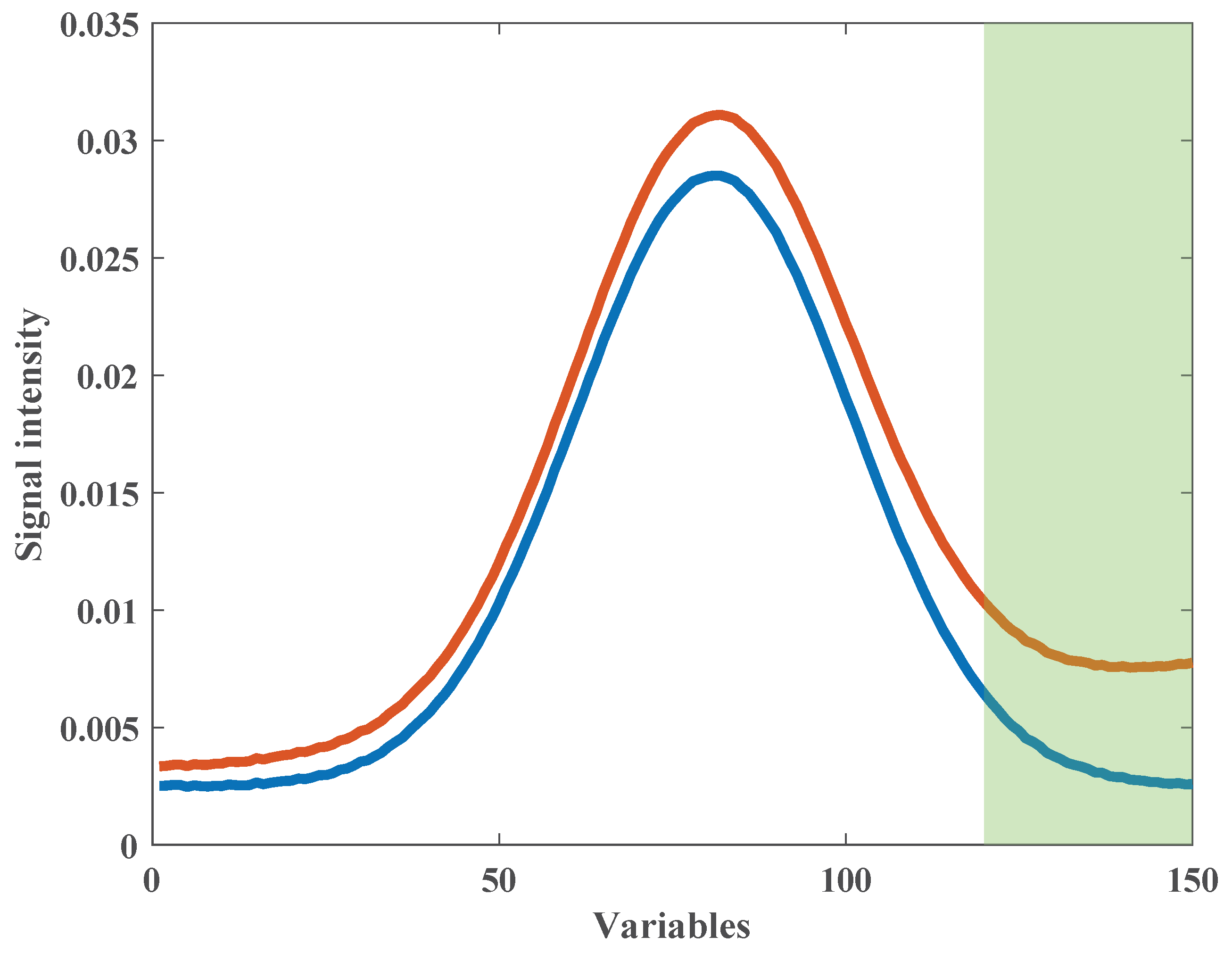
According to Formula (10), it can be inferred that the multiplicative and additive effects result in an intercept error, thereby affecting the calculation result of the correlation coefficient. When d i a i and b i a i are large, significant errors in the correlation coefficient will appear in the latter half of the near-infrared spectral band, which will affect the optimal result F i , x of the dynamic programming optimization algorithm and cause severe distortion of the spectral band output by the COW algorithm. Figure 2 depicts two near-infrared spectra affected by multiplicative and additive effects. From the graph, it can be observed that distortion in the latter half of the spectra significantly impacts the calculation of the correlation coefficients.

2.4. EMSC Algorithm Challenges with Peak Shifts in Spectral Data

Let us assume that the maximum peak of the spectral mean, X m e a n , is located at X m e a n , max in the q-th column. Let us take an ideal spectrum, X i , from the sample set. In reality, when there is an offset in the near-infrared spectrum, there exists an offset spectrum, X i , with an offset of β , which can be represented as x 1 , , x β , X i , α . The length of X i is the same as that of the ideal spectrum X i , and X i , α is the submatrix formed by the first to α columns of the ideal spectrum X i . The peak of X i is located at the ( q + β ) -th column. Substituting the X i and X m e a n spectra into Equations (3) and (4), and rearranging the formula, we obtain:
X i = x 1 , , x β , X i , α = x 1 , , x β , a i X i , α ; c h e m + b i , α I + w i , α λ α + d i , α λ α 2 + ε i , α
The row vector X i , α ; c h e m in Equation (11) is the theoretical absorption spectrum of sample i after being shifted by β bands, and can be represented by Equation (3).
X i , α ; c h e m = p × j = 1 J c i , α , j s j , α , j = 1 , 2 , , J
X i = x 1 , , x β , X i , α = x 1 , , x β , a i p × j = 1 J c i , α , j s j , α + b i , α I + w i , α λ α + d i , α λ α 2 + ε i , α
Represent the average spectrum X m e a n by dividing it into blocks by columns:
X m e a n = x 1 ; m e a n , , x β ; m e a n , X i , α ; m e a n
X i α i X m e a n = x 1 α i x 1 ; m e a n , , x β α i x β ; m e a n , a i p × j = 1 J c i , α , j s j , α + b i , α I + w i , α λ α + d i , α λ α 2 + ε i , α α i X i , α ; m e a n
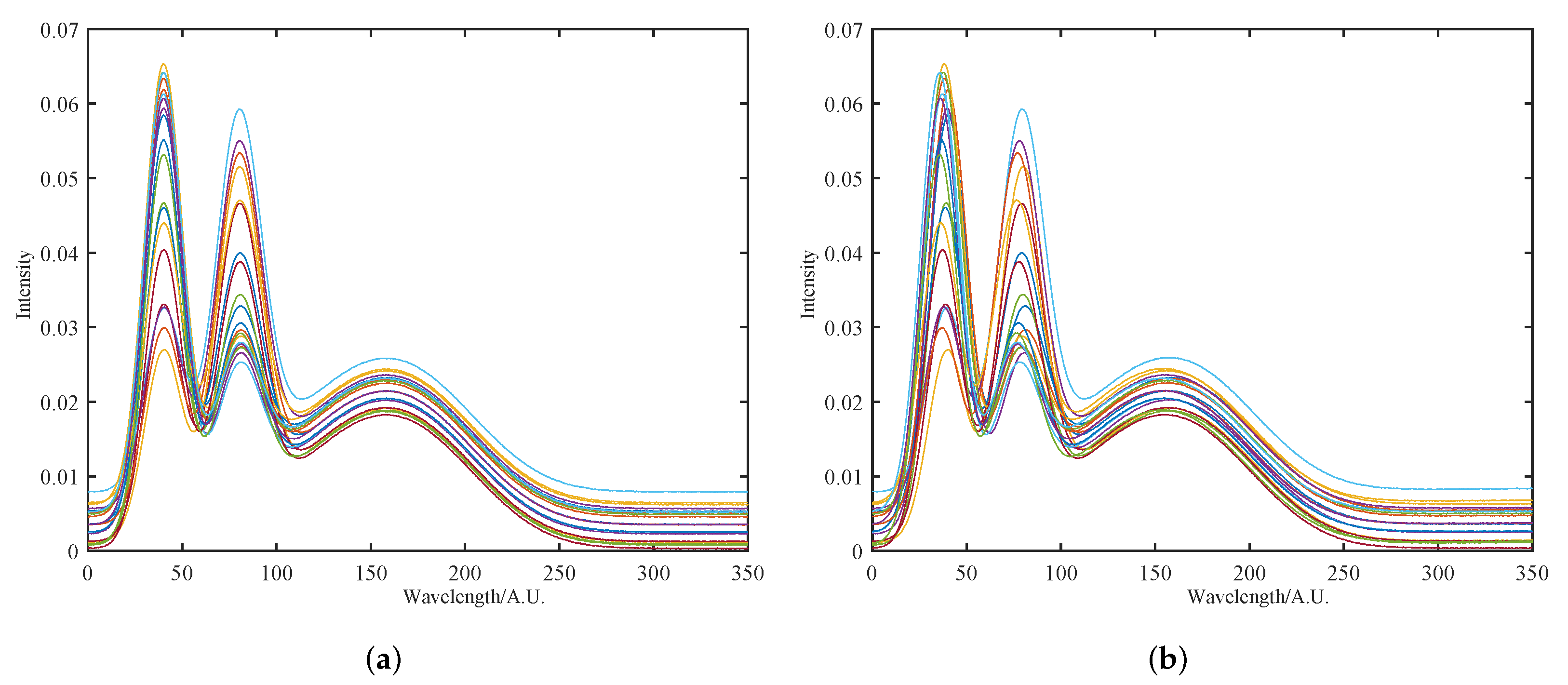
We discovered that, due to spectral shift issues, when using the least squares method to solve, a horizontally shifted error of β will appear in X i α i X m e a n . From an analytical chemistry perspective, we examined the two sets of spectra. The ( β + 1 ) -th band of X i should correspond to the first band, x 1 ; m e a n , of X m e a n after repositioning. We focused on analyzing the spectral bands from the q-th column to the ( q + β ) -th column. At this point, the spectral slope of X i was positive, while the spectral slope of X m e a n was negative. The inconsistency in slopes can cause significant interference in the MSC/SNV calibration results. Furthermore, when dealing with a set of spectra exhibiting peak shifts, the average spectrum X m e a n will also be subject to significant errors. Figure 3 provides a visual representation of the spectra curves affected by the offset. Based on the visual assessment and comparison depicted in Figure 3, the differences in slope between the two sets of spectra can be evaluated.

2.5. SNV Algorithm Challenges with Multiplicative and Additive Effects in Spectral Data

SNV assumes that multiplicative effects are uniform over the whole spectral range [31,32], which is not always the case, particularly when there is a quadratic term, c l + d l 2 , varying with wavenumber in the near-infrared spectra. As mentioned earlier, SNV introduces artifacts to the spectra. This will now be demonstrated through theoretical derivation.
Let the equation for the spectrum after SNV transformation be represented as Equation (16):
x i , j S N V = ( x i , j x ¯ i ) j = 1 p ( x i , j x ¯ i ) 2 p 1
where x i , j S N V is the element of the transformed spectrum, x i , j is the corresponding original element of the spectrum i at variable j, x ¯ i is the mean of spectrum i, and p is the number of variables or wavelengths in the spectrum.
Let the theoretical absorption spectrum unaffected by multiplicative and additive effects be denoted as x i , c h e m . The relationship between the theoretical absorption spectrum and the actual spectrum can be expressed using Equation (17) when the signal is not affected by random measurement noise w i λ + d i λ 2 :
x i = a i x i , c h e m + b i I + ε i
Substituting Equation (17) into Equation (16), we obtain:
x i , j S N V = x i , j x ¯ i j = 1 p x i , j x ¯ i 2 p 1 = a i x i , j ; c h e m + b i I + ε i a i x ¯ i ; c h e m + b i I + ε i j = 1 p a i x i , j ; c h e m + b i I + ε i a i x ¯ i ; c h e m + b i I + ε i 2 p 1 = x i , j ; c h e m x ¯ i ; c h e m j = 1 p x i , j ; c h e m x ¯ i ; c h e m 2 p 1
a i and b i I + ε i can be fully eliminated, resulting in a perfect correction of the additive and multiplicative effects. However, when the signal is affected by random measurement noise w i λ + d i λ 2 , the relationship between the theoretical absorbance spectrum and the actual spectrum can be represented by Equation (19):
x i = a i x i , c h e m + b i I + w i λ + d i λ 2 + ε i
When Equation (19) is substituted into the term x i , j x ¯ i of the SNV method, expanding the term x i , j x ¯ i yields:
a i x i , j ; c h e m + b i I + w i λ i + d i λ i 2 + ε i a i x ¯ i ; c h e m + b i I + w i λ ¯ + d i λ ¯ 2 + ε i
In Equation (20), λ represents wavenumber, and after taking the average, w i λ i + d i λ i 2 cannot be balanced and eliminated with w i λ ¯ + d i λ ¯ 2 , introducing new artifacts to the preprocessed spectrum.

2.6. First Derivative Algorithm Challenges with Multiplicative and Additive Effects in Spectral Data

The first derivative algorithm is a commonly used preprocessing algorithm for near-infrared spectra. It effectively corrects for multiplicative effects and baseline drift [33,34]. However, it is well-known that the first derivative can amplify the noise in the near-infrared spectral signal. Additionally, due to the widespread use of electronic components in near-infrared spectrometers, the amplification circuitry in the sensor can also amplify high-frequency noise while capturing and processing the near-infrared spectral information of the sample [35]. High-frequency noise, caused by the quantum properties of photons in the sensor, is an unavoidable noise source. Therefore, the first derivative algorithm has inherent limitations when applied to near-infrared spectra preprocessing.

3. Materials and Methods

3.1. Spectral Offset Recalibration Method

Based on the aforementioned analysis, existing spectral preprocessing methods are unable to address the complexity arising from the combination of peak shifts and multiplicative and additive effects. Therefore, this study proposes a new preprocessing method called Spectral Offset Recalibration (SOR). The principle of the SOR method can be summarized as follows:
Considering that the COW peak shift method can calculate a set of value functions based on the signal curve and obtain the calibrated spectral signal using these value functions, we leveraged this characteristic in combination with a prior multiplicative and additive effects correction method such as the MSC algorithm. By first applying the multiplicative and additive effects correction to the original spectral signal and then performing the COW peak shift correction, the benefit function values could effectively mitigate the impact of the multiplicative and additive effects. These benefit function values were then applied to the original spectrum, followed by another round of multiplicative and additive effect recalibration, resulting in a more accurate correction for the combined effect of peak shifts and multiplicative and additive effects on the original spectrum. The workflow of the new algorithm is as follows:
  • The matrix M is defined as:
    M = r 1 1 1 1 r 2 1 2 4 r p 1 p p 2
    where r 1 , r 2 , , r p are the coefficients corresponding to the spectral basis functions. This matrix is used in the calculation of the EMSC coefficients and the subsequent coefficient correction in the EMSC method.
  • The Pearson product-moment correlation coefficient is used to calculate the degree of correlation between each spectrum in the original spectrum and the rest of the spectral dataset. These correlation coefficients are then summed and normalized to obtain the weight vector, denoted as W, for the EMSC method. The calculation formula for the weight vector is as follows:
    ρ i = ρ x i ; x 1 , , x i 1 , x i + 1 , x p = j = 1 p c o v x i , x j σ x i σ x j j i
    W = i = 1 p ρ i
  • To calculate the EMSC coefficients, denoted as
    a b c d = M W M T 1 M W x T
    where X is a matrix representing the original spectra, with dimensions N × L , where L is the number of spectral data points; T denotes matrix transpose.
  • The coefficient-corrected signal can be obtained using the formula:
    z = 1 a x 1 1 1 1 2 4 1 p p 2 b a c a d a
    where:
    • x represents the original spectrum.
    • a, b, c, and d are the EMSC coefficients obtained from the previous step.
    • The matrix represents the matrix of spectral basis functions, with p indicating the number of basis functions used.
  • Let us define the alignment quality, also known as the gain function, as the correlation coefficient ρ between the corrected spectrum z and the spectrum average. The gain function is denoted as f ( I ) and is measured as f ( I ) = ρ ( I T , I A ) , where I represents the segment number. The gain function is defined by the formula:
    z ¯ = arg max z i = 0 N 1 f z i ; z i + 1
    Here, the i-th segment of the spectrum z i ; z i + 1 is defined by the boundary points z i and z i + 1 . Given z 0 = 0 < z 1 < < z N 1 < z N = L T and u i [ Δ t , Δ + t ] ; i = 0 , , N 1 , where Δ is a constant and t is the tolerance, we have z i + 1 = z i + m + u i ; i = 0 , , N 1 .
  • To correct the original spectrum x based on the optimal gain function, we can follow these steps:
    • Define the boundary points z i based on the desired segmentation of the spectrum: z 0 = 0 , z 1 , z 2 , …, z N 1 , z N = L T .
    • Determine the values of u i within the range [ Δ t , Δ + t ] for each segment, where u i represents the offset or shift to be applied to the corresponding segment. Here, Δ is a constant and t is the tolerance.
    • Calculate the corrected spectrum x ¯ by applying the following equation for each segment i: x ¯ = a r g max x i = 0 N 1 f x i ; x i + 1 , where x i ; x i + 1 denotes the section defined by border points x i and x i + 1 .
    • Repeat the above step for all segments of the spectrum.
    By applying this correction process based on the optimal gain function, the original spectrum x can be effectively aligned and corrected.
  • To further process the offset-corrected near-infrared spectra using the EMSC method, the influence of multiplicative scatter effects are mitigated and further processed spectra for analysis or comparison are obtained.

3.2. Processing Chart Summary

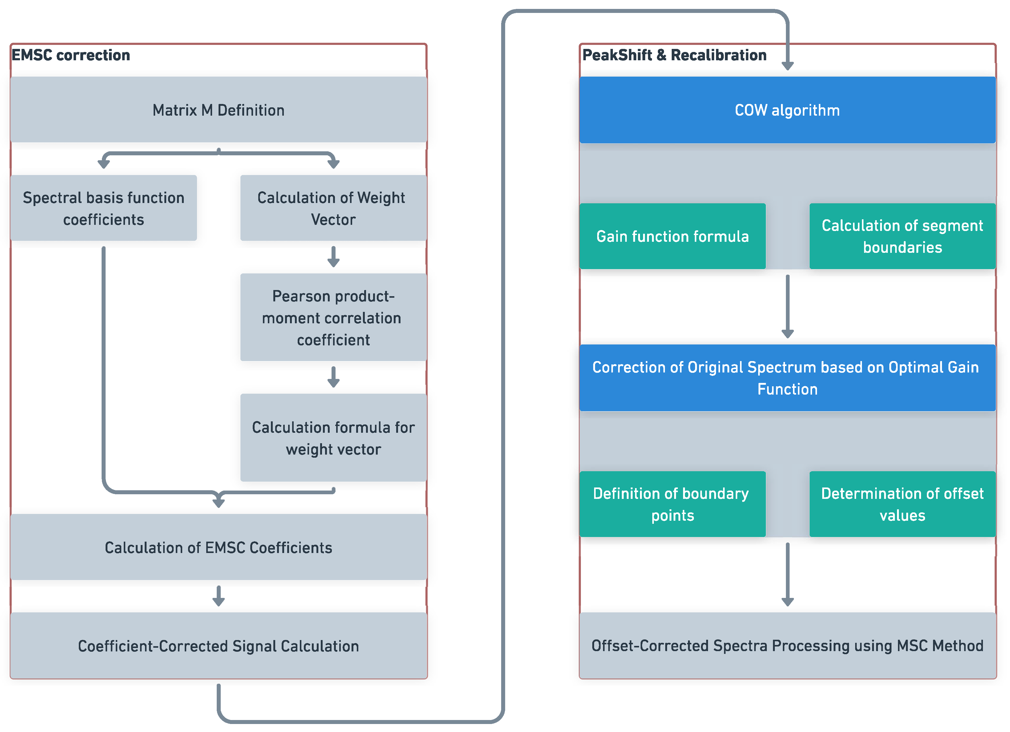
This section presents a brief flowchart of the SOR method, where the key steps and their applications discussed in the brief flowchart are described in Section 3.1. The Figure 4 illustrates the SOR method for coefficient correction and alignment of near-infrared spectra, aiming to provide a clear foundation for subsequent content.

3.3. Simulated Spectra

The simulated spectrum was composed of three Gaussian distributions with a total of 700 spectral bands. The weights for these distributions were randomly sampled from a uniform distribution between 0 and 1. Figure 5a illustrates the three Gaussian-shaped spectral peaks.
Next, these three Gaussian distributions were linearly combined to create a simulated spectrum signal. The resulting signal is shown in Figure 5b. The means of the three Gaussian distributions were 40, 80, and 170, with standard deviations of 10, 12, and 4, respectively.
Subsequently, the spectra were multiplied by a scalar, which was randomly drawn from a normal distribution with a mean of 1 and a standard deviation of 0.1. The multiplied spectra were then added with a background structure and white noise. The background structure was at a scale of 0.1% of the signal, while the white noise was at a scale of 0.001% of the signal. The white noise was generated from a normal distribution with a mean of 0. The resulting spectra are shown in Figure 6a.
Finally, an additional term of c l + d l 2 was added to these spectra and offset noise was added to the spectral curves, where c and d follow normal distributions with zero mean and standard deviations of 3.7 9 and 2.6 8 , and l represents the number of spectral bands, respectively. The resulting signal is shown in Figure 6b.

3.4. NIR Spectra of Wood

This dataset comprises near-infrared spectra of solid wood veneers. The near-infrared spectra were acquired using a portable NIRS (InGaAs)-array spectrometer (NIRquest512, Orlando, FL, USA). The spectrometer’s parameters were as follows: the detection range began at 900 nm and ended at 1700 nm, with an average interval of 3.1 nm between spectral bands. The user interface for the near-infrared spectrometer was the SpectraSuite 2.0 (Quadrangle Blvd, Orlando, FL, USA) spectroscopy software platform.

4. Result and Discussion

4.1. Simulated Spectra

4.1.1. Initial Multiplicative and Additive Effect Correction Results Using SOR Method

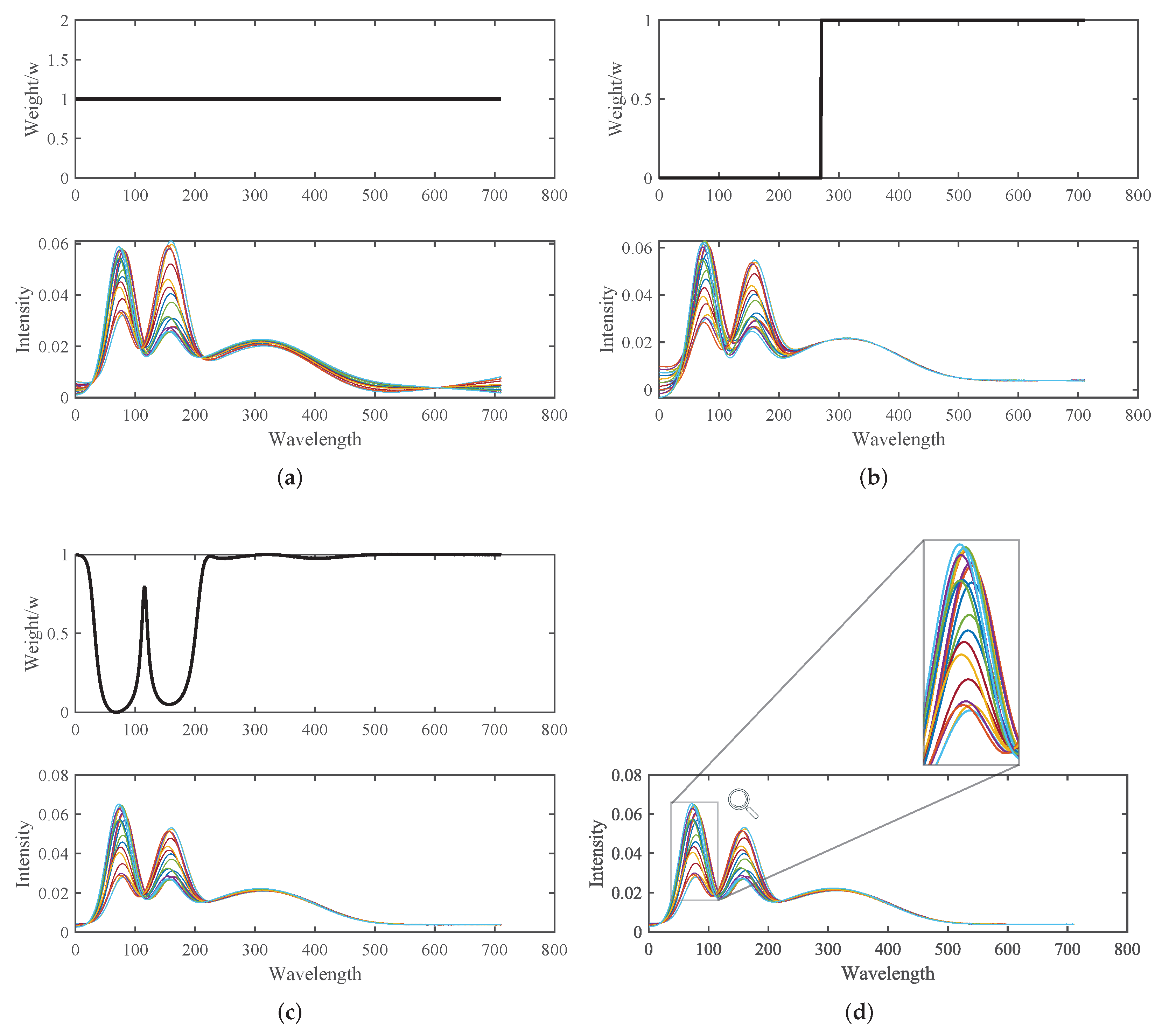
Figure 7 illustrates the results obtained by applying three preprocessing methods to near-infrared simulated spectra affected by multiplication factors and baseline drift (as shown in Figure 6a). The three methods include the weighted MSC algorithm, with a weight vector of all ones (Figure 7a); the weighted MSC algorithm, with manually set weights (Figure 7b); and the SOR recalibration method (Figure 7c).
In the weighted MSC algorithm shown in Figure 7a (top), the weights were set to a vector of all ones. In Figure 7b (top), the weights were manually set, with zeros in the region covering two chemical peaks (from 0 to 270) and unity in the rest of the spectral range (from 271 to 700). Figure 7c (top) represents the weights obtained through the SOR recalibration method, resulting in a smooth and distinct weight spectrum.
The spectra were processed for Initial Correction using the SOR algorithm based on the all-ones matrix, as shown in Figure 7a. The spectra in the range of 0–270 represent the linear combination of the first two peaks. However, the all-ones matrix yielded the poorest results among the three approaches. Figure 7d presents the spectra processed by the weighted MSC algorithm, where it can be observed that the offset issue persists. This may be attributed to the significant bias introduced by the all-ones weighted MSC matrix.
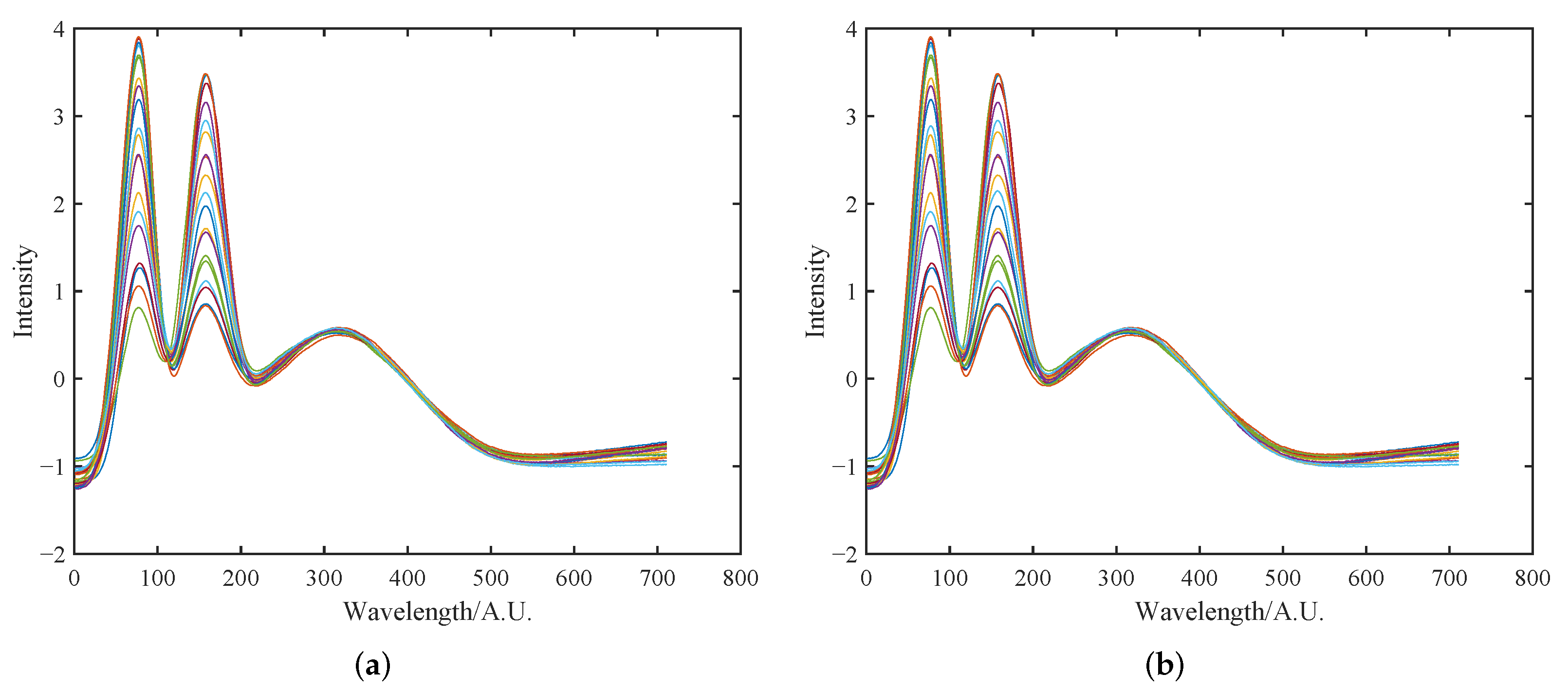
In contrast, Figure 7b represents the spectra processed using the ideal weight matrix (W) generated based on the simulated spectral characteristics, while the spectra in the range of 271–700 serve as a reference spectrum unaffected by shape effects. Therefore, the weight values were set to 0 for the first two peaks in the range of 0–270 and set to 1 for the peaks in the range of 271–700. The SOR algorithm constructed using this matrix produced the spectra shown in Figure 7b. Significant differences can be observed between these spectra. The two chemical peaks of the ideal spectra exhibit similar changes and have similar maximum values. In practice, for a set of real near-infrared spectra, the variance is often concentrated in specific regions of the spectrum, while the standard MSC transformation applies uniform normalization to all variables.
Figure 7b,c employ the weighted MSC algorithm. In both figures, the weights are close to 0 in the region affected by shape effects (0–271) and nonzero in the region affected only by size effects (271–700). The weighted MSC algorithm utilized these weights to calculate the mean and standard deviation of the spectra, mainly located in the right region. In the ideal case of Figure 7b, it can be directly observed that the algorithm calculated the mean and standard deviation of only the spectra affected by size effects during variable selection, leading to excellent spectral preprocessing results. Figure 7c, on the other hand, determines the values of matrix W based on the correlation coefficients of the near-infrared spectra (correlation coefficient method). When the diagonal values of W corresponding to a specific wavelength are large, the average and standard deviation of the spectral variables for the current wavelength have a high correlation with the results of the SOR algorithm. Both weighting approaches effectively estimate the multiplicative and additive factors, as shown in Figure 7c. Although the spectral preprocessing results in Figure 7c are not as good as the ideal case in Figure 7b, it is because the ideal weight matrix (W) was generated based on the simulated spectral characteristics of the experiment. However, for a set of unknown test samples, the correlation coefficient method used in the results of Figure 7c can achieve near-perfect calibration.

4.1.2. Peak Shift Correction and Recalibration Results Using SOR Method

Building upon the COW alignment theory, we extended our methodology by incorporating an alignment and calibration step to further enhance the quality of preprocessing. After undergoing initial calibration using the SOR algorithm, the simulated spectra were subjected to COW alignment, which involved segmenting the spectra into individual segments and assessing their distortion levels. Subsequently, an objective function was computed, which informed the offset correction of the original spectra.
Figure 8 provides a visual representation of the original spectral segments before and after alignment using COW. The alignment process yielded satisfactory results, aligning peak maximums with positions in the reference spectrum. However, the influence of multiplicative effects introduced some inaccuracies in the aligned signals. Notably, translation induced by the alignment algorithm can lead to deformation in peaks affected by size effects, resulting in concavity issues at peak crests in certain regions (420–500 nm).
Finally, the SOR algorithm’s recalibration step was employed to eliminate both multiplicative and additive effects from the spectrum. After addressing peak shifts and ensuring minimal impact on the original spectrum, the removal of multiplicative and additive effects becomes a straightforward task. Figure 9 showcases the final outcome following the SOR algorithm’s corrective process, exemplifying the successful removal of these effects.

4.1.3. Comparative Analysis of Preprocessing Method Results and Performance

In continuation of the principles outlined in the VSN paper [25], we extended our exploration in Section 3.3 by introducing a unique strategy aimed at overcoming the inherent challenge of quantitatively gauging the effectiveness of preprocessing algorithms when conventional metrics are absent within the realm of near-infrared spectroscopy. Our approach involved the formulation of an innovative methodology centered around the creation of specialized simulated spectra. These simulated spectra were specifically crafted to counteract the limitations of traditional efficacy evaluation. They served as controlled testbeds, intricately tailored to mimic complex scenarios wherein spectral characteristics are intentionally altered, thereby facilitating a comprehensive assessment of preprocessing algorithm performance.
As illustrated in Figure 6, this set of simulated spectra operated within the 0–270 wavenumber range, where two distinct peak groups were scaled by varying coefficients according to the pattern of Linear Combinations of Normal Random Variables. A third peak remained unaltered by multiplicative scaling. Subsequently, drift noise and peak shift errors were introduced to these simulated spectra.
The efficacy of preprocessing algorithms is traditionally challenging to quantify in near-infrared spectroscopy due to the lack of standardized metrics. In lieu of conventional evaluation criteria, we employed this specialized set of simulated spectra as a surrogate for performance assessment. The width of the third peak served as an indicator of algorithmic effectiveness, with narrower peaks signifying superior performance. We evaluated the efficacy of SNV, MSC, EMSC, and the proposed SOR algorithm on this simulated dataset, aiming to discern the preprocessing approach that yielded the most favorable results. Notably, a narrower third peak indicated better algorithmic performance.
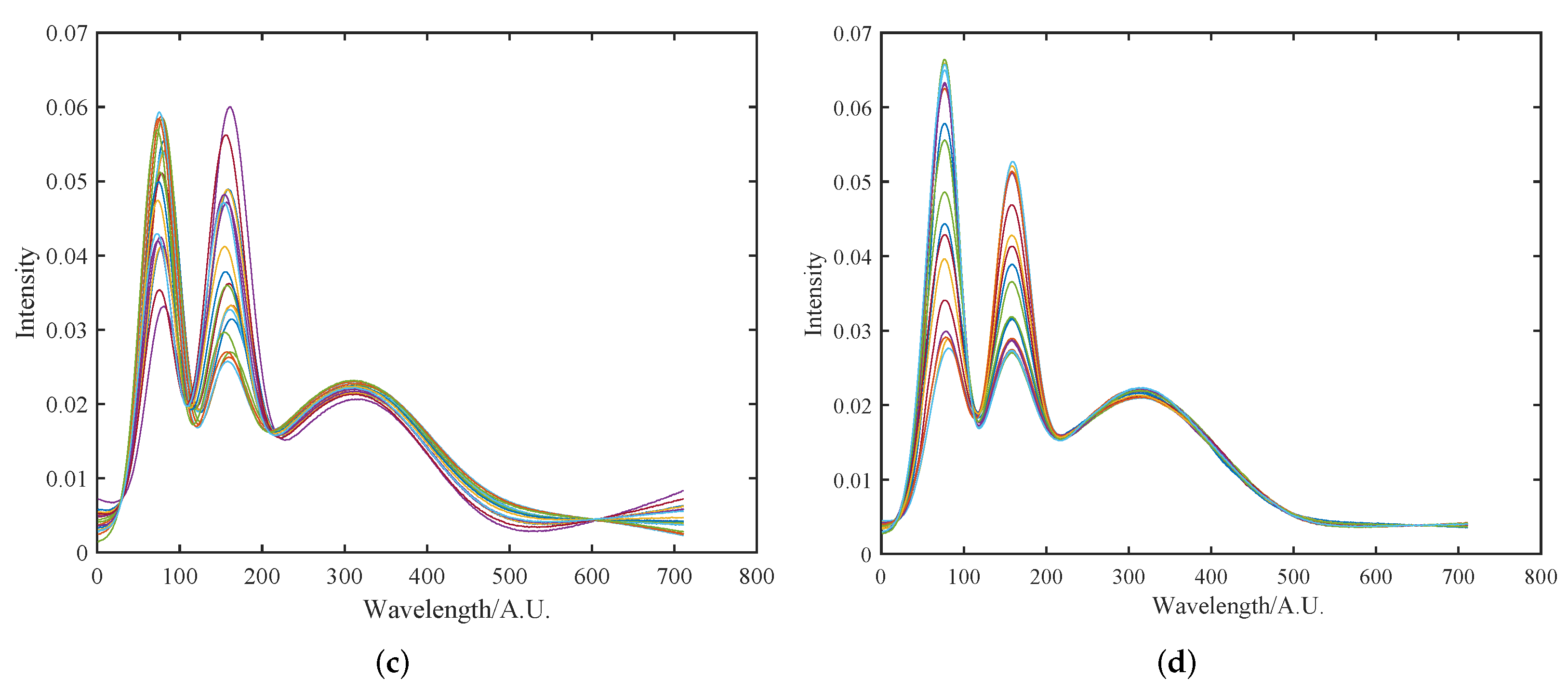
Figure 9 depicts the near-infrared spectra processed by the four preprocessing algorithms: SNV-COW, MSC-COW, EMSC-COW, and our proposed SOR algorithm. Evidently, the third peak of the spectra processed by SNV and MSC still exhibited some degree of drift. Notably, the EMSC algorithm seemed to introduce distortions even more pronounced than those observed with SNV. In contrast, the preprocessing results obtained with our proposed SOR algorithm exhibited superior performance in addressing these distortions.

4.2. NIR Spectra of Wood

4.2.1. Initial Multiplicative and Additive Effect Correction Results Using SOR Method

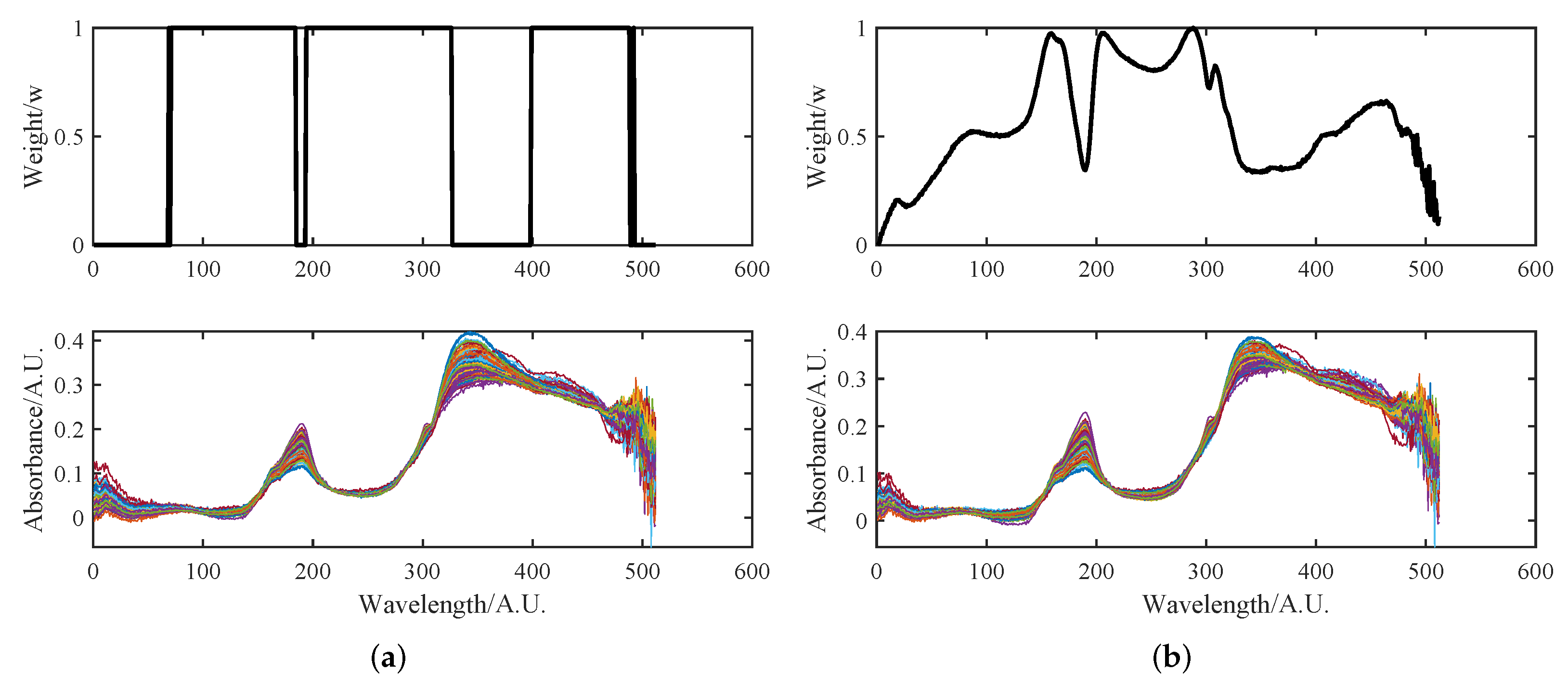
Figure 10 illustrates the processing results of the near-infrared spectra of solid wood panels, which are clearly affected by baseline offset and multiplicative effects. The results of EMSC are shown in Figure 10a, where the baseline and multiplicative effects are significantly reduced. However, due to the impact of spectral peak shift effects, the correction of the peaks at 191 nm and 336 nm is less satisfactory. In Figure 10b, manually selected weights were used to exclude the portions expected to provide information from the EMSC calculations. The weights were set to 0 at the positions of the characteristic peaks and to 1 for the other wavelengths. Similarly, based on the correlation coefficients of the near-infrared spectra, the values of matrix W were determined for the weighted EMSC. The results of the weighted EMSC are shown in Figure 10b. The side effects of EMSC have been eliminated, and the positions of the peaks and valleys in the spectrum are well-separated, while remaining very close in the rest of the wavelength range.

4.2.2. Peak Shift Correction and Recalibration Results Using SOR Method

After the preliminary preprocessing of the NIR spectra of solid wood panels using Initial Correction for the SOR Method, the multiplicative effects in the spectra were effectively corrected, thereby eliminating their influence on the peak shift algorithm. Subsequently, in this study, the average spectrum of this dataset was taken as the reference baseline for the NIR spectra, and the Peak shift Correction algorithm was employed to construct a cost function. This cost function included the optimal distortion of the reference samples. Based on this cost function, the original NIR spectra of uncorrected solid wood panels were aligned. To visualize a portion of the original spectra graph (range: 0–512), Figure 11 serves as an example, demonstrating the effect of the Peak shift Correction algorithm on the spectral peak alignment of the simulated spectral data. The alignment effect is satisfactory, with the peak maximum values aligned to the positions in the reference spectrum.
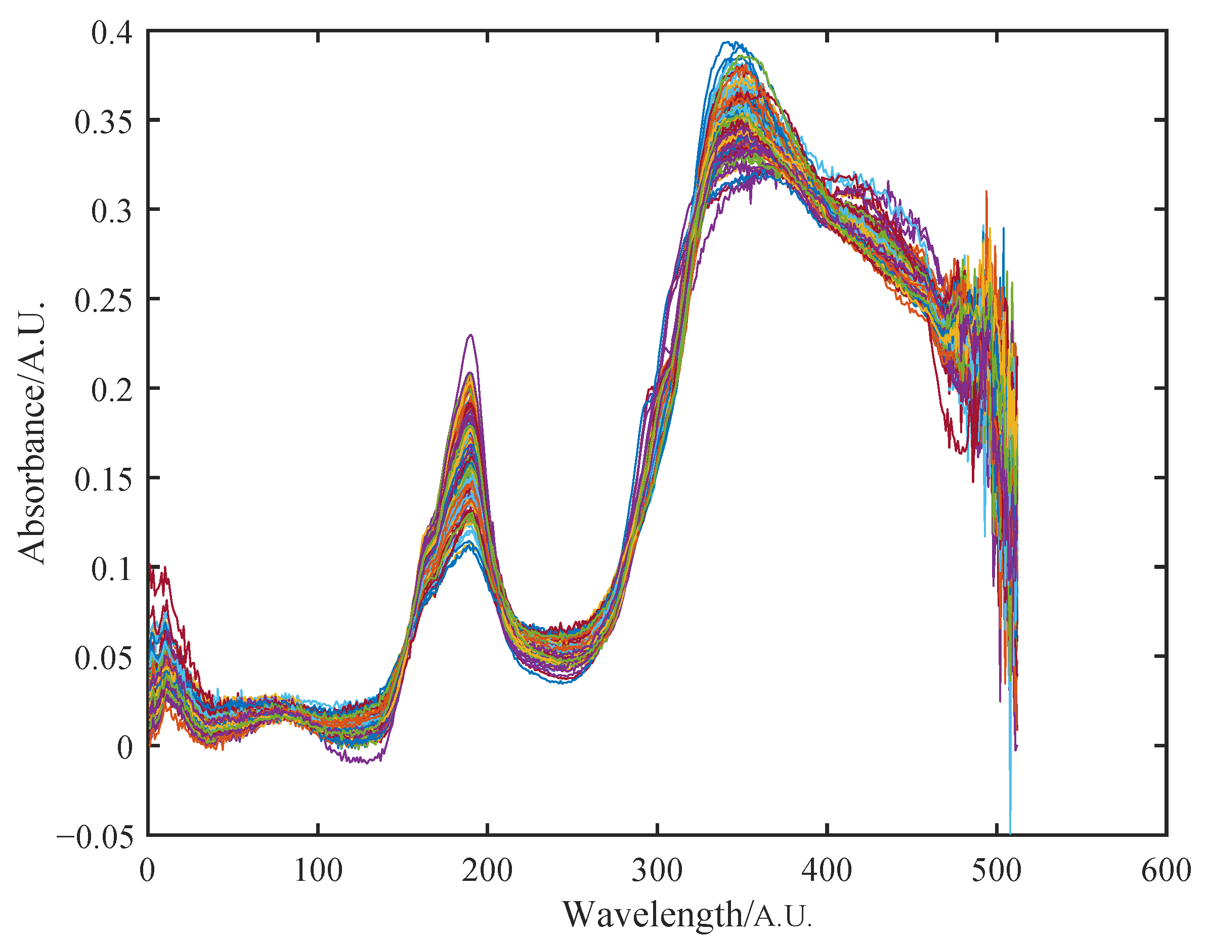
Satisfactory alignment can be observed for the first and second characteristic peaks of the spectral signal. However, minor inaccuracies were detected near point 190 in the spectrum graph. Some changes in the shape of the absorption peak were observed in the vicinity of this wavelength range. Additionally, the position where the feature peak should be located at 350 was not entirely satisfactory. Nevertheless, these feature peaks at these positions have relatively low intensities and do not belong to the spectral bands that primarily reflect the mechanical properties and other main attributes of the wood. Hence, they can be disregarded. After the initial offset correction of the raw spectra, the MSC algorithm was employed for recalibration, and Figure 12 represents the final recalibration result.

5. Conclusions

In this study, we developed a new algorithm based on the combination of the EMSC and COW algorithms address the complex issues arising from the coupling of additive and multiplicative effects with signal shift in multivariate signals. The application of the new algorithm effectively corrected peak shifts and drift problems in the original spectra, as demonstrated on both simulated and real data.
However, it is important to further emphasize specific issues related to the use of the new algorithm. Firstly, when facing square drift and shape effects in near-infrared spectroscopy, the SNV algorithm exhibited poor data performance after preprocessing, while the first derivative algorithm suffered from high noise levels. The new algorithm abandoned these preprocessing methods targeting individual signals and required the definition of a “learning set” to compute the weight matrix. Nevertheless, this is not a major concern, as such learning sets are typically required in successive stages of model construction.
Furthermore, several aspects need further investigation to achieve a fully automated implementation of the algorithm. One such aspect is the design of parameters in the weight generation function. Although a weight calculation method based on the sigmoid function transformation was proposed, its theoretical support is currently insufficient and requires validation on other datasets, similar to the validation performed on a real dataset of wood spectra. The impact of other tunable parameters in COW may also warrant additional investigation, which can be addressed through theoretical research.
Lastly, it should be noted that the new algorithm does not provide any improvement compared to standard normalization methods when dealing with multivariate data where shape effects are present in all variables and no square offset term exists. In such cases, the combination of the SNV method with the COW offset-correction algorithm can be used as an alternative preprocessing approach to the new algorithm.
In conclusion, the proposed algorithm effectively addresses the complex issues arising from the coupling of additive and multiplicative effects with signal shift in multivariate spectroscopic analysis. However, further research is needed to address specific issues related to the algorithm’s usage and to achieve fully automated implementation. By considering these aspects, the algorithm can be further enhanced and applied to a wide range of spectroscopic datasets, enabling accurate and reliable analysis in various scientific and industrial applications.

Author Contributions

Conceptualization, D.J. and Y.Z.; methodology, D.J.; software, D.J.; validation, D.J.; formal analysis, D.J.; investigation, D.J.; resources, Y.Z.; data curation, Y.G.; writing—original draft preparation, D.J.; writing—review and editing, D.J.; visualization, D.J.; supervision, K.W.; project administration, K.W.; funding acquisition, Y.Z. All authors have read and agreed to the published version of the manuscript.

Funding

This work was supported financially by the China State Forestry Administration “948” projects (2015-4-52), Heilongjiang Natural Science Foundation (C2017005).

Institutional Review Board Statement

Not applicable.

Informed Consent Statement

Not applicable.

Data Availability Statement

The data presented in this study are not publicly available due to restrictions such as privacy or ethical concerns. The near-infrared spectroscopy data related to wood are collected by our team in the laboratory.

Conflicts of Interest

The authors declare no conflict of interest. The funders had no role in the design of the study; in the collection, analyses, or interpretation of data; in the writing of the manuscript; or in the decision to publish the results.

Abbreviations

The following abbreviations are used in this manuscript:
EMSCExtended Multiplicative Signal Correction
COWCorrelation-Optimized Warping
NIRnear-infrared
LC-MSliquid chromatography-mass spectrometry
GC-MSgas chromatography-mass spectrometry
NIRSnear-infrared spectroscopy
MSCmultiplicative signal correction
SNVstandard normal variate
DTWDynamic Time Warping
SORSpectral Offset Recalibration

References

  1. Ríos-Reina, R.; Azcarate, S.M. How chemometrics revives the UV-Vis spectroscopy applications as an analytical sensor for spectralprint (nontargeted) analysis. Chemosensors 2023, 11, 8. [Google Scholar] [CrossRef]
  2. Sorochan Armstrong, M.D.; de la Mata, A.P.; Harynuk, J.J. Review of variable selection methods for discriminant-type problems in chemometrics. Front. Anal. Sci. 2022, 2, 867938. [Google Scholar] [CrossRef]
  3. Rajendran, H.K.; Fakrudeen, M.A.D.; Chandrasekar, R.; Silvestri, S.; Sillanpaa, M.; Padmanaban, V.C. A comprehensive review on analytical and equation derived multivariate chemometrics for the accurate interpretation of the degradation of aqueous contaminants. Environ. Technol. Innov. 2022, 28, 102827. [Google Scholar] [CrossRef]
  4. Dayananda, B.; Owen, S.; Kolobaric, A.; Chapman, J.; Cozzolino, D. Pre-processing applied to instrumental data in analytical chemistry: A brief review of the methods and examples. Crit. Rev. Anal. Chem. 2023. [Google Scholar] [CrossRef] [PubMed]
  5. Trinklein, T.J.; Cain, C.N.; Ochoa, G.S.; Schöneich, S.; Mikaliunaite, L.; Synovec, R.E. Recent advances in GC×GC and chemometrics to address emerging challenges in nontargeted analysis. Anal. Chem. 2023, 95, 264–286. [Google Scholar] [CrossRef] [PubMed]
  6. Wu, Y.; Peng, S.; Xie, Q.; Han, Q.; Zhang, G.; Sun, H. An improved weighted multiplicative scatter correction algorithm with the use of variable selection: Application to near-infrared spectra. Chemom. Intell. Lab. Syst. 2019, 185, 114–121. [Google Scholar] [CrossRef]
  7. Mishra, P.; Biancolillo, A.; Roger, J.M.; Marini, F.; Rutledge, D.N. New data preprocessing trends based on ensemble of multiple preprocessing techniques. TrAC Trends Anal. Chem. 2020, 132, 116045. [Google Scholar] [CrossRef]
  8. Bloemberg, T.G.; Gerretzen, J.; Lunshof, A.; Wehrens, R.; Buydens, L.M. Warping methods for spectroscopic and chromatographic signal alignment: A tutorial. Anal. Chim. Acta 2013, 781, 14–32. [Google Scholar] [CrossRef]
  9. Zhang, W.; Kasun, L.C.; Wang, Q.J.; Zheng, Y.; Lin, Z. A review of machine learning for near-infrared spectroscopy. Sensors 2022, 22, 9764. [Google Scholar] [CrossRef]
  10. Li, S.; Viscarra Rossel, R.A.; Webster, R. The cost-effectiveness of reflectance spectroscopy for estimating soil organic carbon. Eur. J. Soil Sci. 2022, 73, e13202. [Google Scholar] [CrossRef]
  11. Beć, K.B.; Grabska, J.; Huck, C.W. Miniaturized NIR spectroscopy in food analysis and quality control: Promises, challenges, and perspectives. Foods 2022, 11, 1465. [Google Scholar] [CrossRef]
  12. Kim, J.; Hwang, W.S.; Kim, D.; Kim, D.Y. Fast noniterative data analysis method for frequency-domain near-infrared spectroscopy with the microscopic Beer–Lambert law. Opt. Commun. 2022, 520, 128417. [Google Scholar] [CrossRef]
  13. Mishra, P.; Roger, J.M.; Rutledge, D.N.; Woltering, E. SPORT pre-processing can improve near-infrared quality prediction models for fresh fruits and agro-materials. Postharvest Biol. Technol. 2020, 168, 111271. [Google Scholar] [CrossRef]
  14. Yu, H.; Guo, L.; Kharbach, M.; Han, W. Multi-way analysis coupled with near-infrared spectroscopy in food industry: Models and applications. Foods 2021, 10, 802. [Google Scholar] [CrossRef]
  15. Thygesen, L.G.; Lundqvist, S.O. NIR measurement of moisture content in wood under unstable temperature conditions. Part 2. Handling temperature fluctuations. J. Near Infrared Spectrosc. 2000, 8, 191–199. [Google Scholar] [CrossRef]
  16. Watari, M.; Ozaki, Y. Calibration models for the vinyl acetate concentration in ethylene-vinyl acetate copolymers and its on-Line monitoring by near-infrared spectroscopy and chemometrics: Use of band shifts associated with variations in the vinyl acetate concentration to improve the models. Appl. Spectrosc. 2005, 59, 912–919. [Google Scholar] [CrossRef]
  17. Kelly, J.J.; Kelly, K.A.; Barlow, C.H. Tissue temperature by near-infrared spectroscopy. In Proceedings of the Optical Tomography, Photon Migration, and Spectroscopy of Tissue and Model Media: Theory, Human Studies, and Instrumentation; Chance, B., Alfano, R.R., Eds.; International Society for Optics and Photonics: Bellingham, WA, USA, 1995; Volume 2389, pp. 818–828. [Google Scholar] [CrossRef]
  18. Khosravi, M.; Soleimanmeigouni, I.; Ahmadi, A.; Nissen, A. Reducing the positional errors of railway track geometry measurements using alignment methods: A comparative case study. Measurement 2021, 178, 109383. [Google Scholar] [CrossRef]
  19. Khosravi, M.; Soleimanmeigouni, I.; Ahmadi, A.; Nissen, A.; Xiao, X. Modification of correlation optimized warping method for position alignment of condition measurements of linear assets. Measurement 2022, 201, 111707. [Google Scholar] [CrossRef]
  20. Skov, T.; van den Berg, F.; Tomasi, G.; Bro, R. Automated alignment of chromatographic data. J. Chemom. 2006, 20, 484–497. [Google Scholar] [CrossRef]
  21. Wang, S.; Yao, J.; Liu, J.; Petrick, N.; Van Uitert, R.L.; Periaswamy, S.; Summers, R.M. Registration of prone and supine CT colonography scans using correlation optimized warping and canonical correlation analysis. Med. Phys. 2009, 36, 5595–5603. [Google Scholar] [CrossRef]
  22. Li, L.; Peng, Y.; Li, Y.; Wang, F. A new scattering correction method of different spectroscopic analysis for assessing complex mixtures. Anal. Chim. Acta 2019, 1087, 20–28. [Google Scholar] [CrossRef] [PubMed]
  23. Martens, H.; Nielsen, J.P.; Engelsen, S.B. Light scattering and light absorbance separated by extended multiplicative signal correction. Application to near-infrared transmission analysis of powder mixtures. Anal. Chem. 2003, 75, 394–404. [Google Scholar] [CrossRef]
  24. Afseth, N.K.; Kohler, A. Extended multiplicative signal correction in vibrational spectroscopy—A tutorial. Chemom. Intell. Lab. Syst. 2012, 117, 92–99. [Google Scholar] [CrossRef]
  25. Rabatel, G.; Marini, F.; Walczak, B.; Roger, J.M. VSN: Variable sorting for normalization. J. Chemom. 2020, 34, e3164. [Google Scholar] [CrossRef]
  26. Kucha, C.T.; Liu, L.; Ngadi, M.; Gariépy, C. Prediction and visualization of fat content in polythene-packed meat using near-infrared hyperspectral imaging and chemometrics. J. Food Compos. Anal. 2022, 111, 104633. [Google Scholar] [CrossRef]
  27. Haddad, F.; Boudet, S.; Peyrodie, L.; Vandenbroucke, N.; Poupart, J.; Hautecoeur, P.; Chieux, V.; Forzy, G. Oligoclonal band straightening based on optimized hierarchical warping for multiple sclerosis diagnosis. Sensors 2022, 22, 724. [Google Scholar] [CrossRef]
  28. Solheim, J.H.; Zimmermann, B.; Tafintseva, V.; Dzurendová, S.; Shapaval, V.; Kohler, A. The use of constituent spectra and weighting in extended multiplicative signal correction in infrared spectroscopy. Molecules 2022, 27, 1900. [Google Scholar] [CrossRef]
  29. Khodabakhshian, R.; Seyedalibeyk Lavasani, H.; Weller, P. A methodological approach to preprocessing FTIR spectra of adulterated sesame oil. Food Chem. 2023, 419, 136055. [Google Scholar] [CrossRef]
  30. Joshi, P.; Pahariya, P.; Al-Ani, M.F.; Choudhary, R. Monitoring and prediction of sensory shelf-life in strawberry with ultraviolet-visible-near-infrared (UV-VIS-NIR) spectroscopy. Appl. Food Res. 2022, 2, 100123. [Google Scholar] [CrossRef]
  31. Wang, Y.; Ren, Z.; Li, M.; Lu, C.; Deng, W.W.; Zhang, Z.; Ning, J. From lab to factory: A calibration transfer strategy from HSI to online NIR optimized for quality control of green tea fixation. J. Food Eng. 2023, 339, 111284. [Google Scholar] [CrossRef]
  32. Yuan, H.; Liu, C.; Wang, H.; Wang, L.; Dai, L. PLS-DA and Vis-NIR spectroscopy based discrimination of abdominal tissues of female rabbits. Spectrochim. Acta Part A Mol. Biomol. Spectrosc. 2022, 271, 120887. [Google Scholar] [CrossRef] [PubMed]
  33. Huang, J.; He, H.; Wang, L.; Xu, Y.; Song, Z.; Wang, X.; Wang, X. Assessment of total glycerol core aldehyde and monomer content based on NIR and PLS. J. Food Compos. Anal. 2023, 123, 105526. [Google Scholar] [CrossRef]
  34. Malvandi, A.; Kapoor, R.; Feng, H.; Kamruzzaman, M. Non-destructive measurement and real-time monitoring of apple hardness during ultrasonic contact drying via portable NIR spectroscopy and machine learning. Infrared Phys. Technol. 2022, 122, 104077. [Google Scholar] [CrossRef]
  35. Scholkmann, F.; Kleiser, S.; Metz, A.J.; Zimmermann, R.; Mata Pavia, J.; Wolf, U.; Wolf, M. A review on continuous wave functional near-infrared spectroscopy and imaging instrumentation and methodology. NeuroImage 2014, 85, 6–27. [Google Scholar] [CrossRef]
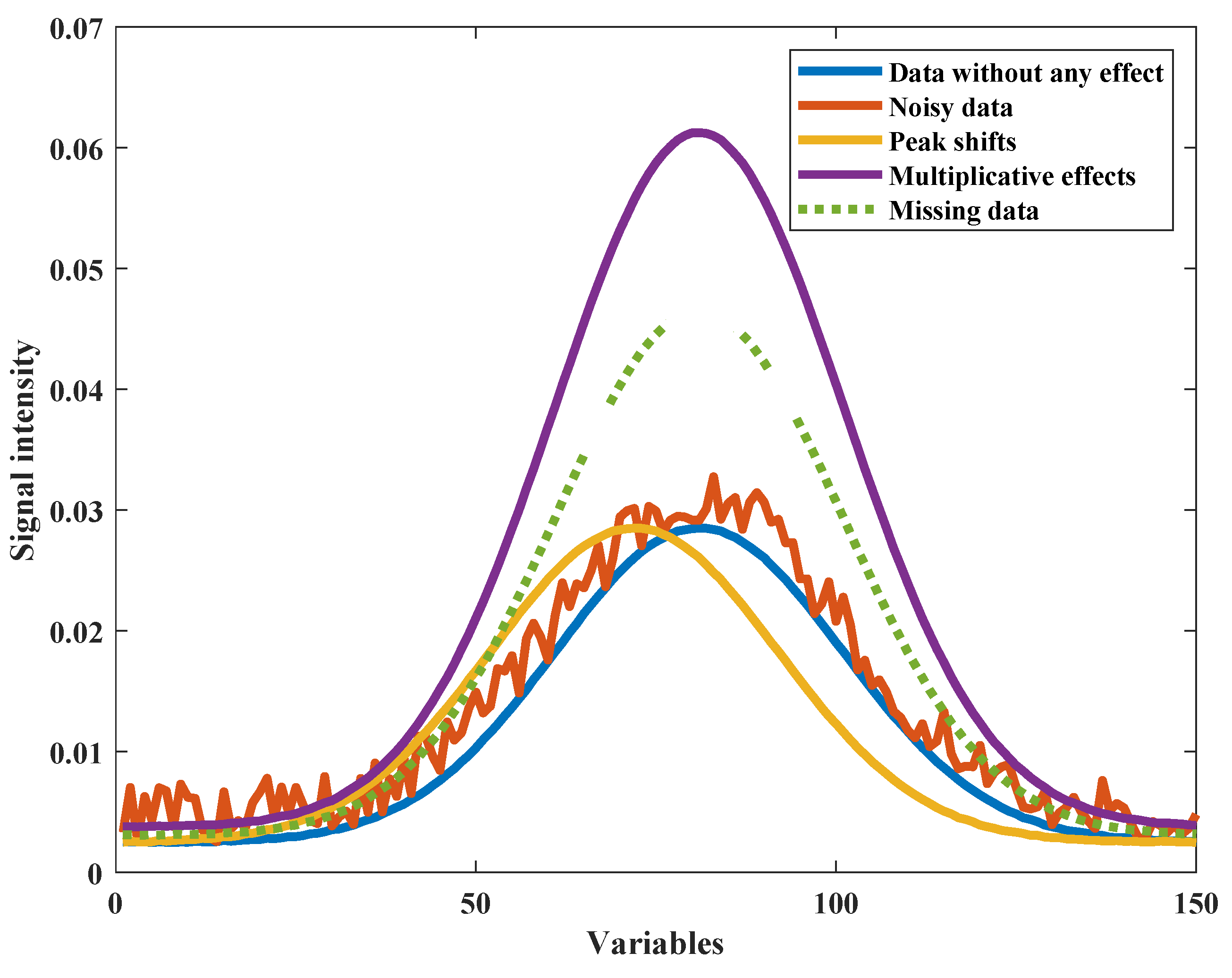
Figure 1. Example of several simulated artefacts for visible and near-infrared data.
Chemosensors 11 00472 g001
Figure 2. Two near-infrared spectra affected by multiplicative and additive effects.
Chemosensors 11 00472 g002
Figure 3. The spectra curves of two sets affected by the offset.
Chemosensors 11 00472 g003
Figure 4. SOR method for spectral coefficient correction and alignment of near-infrared spectra.
Chemosensors 11 00472 g004
Figure 5. Two panels should be listed as: (a) spectra of the three pure components; (b) spectra obtained via linear combination of the three components.
Chemosensors 11 00472 g005
Figure 6. Two panels should be listed as: (a) spectra affected by multiplicative and additive effects and a horizontal baseline; (b) spectra affected by multiplicative and additive effects and a parabolic baseline.
Chemosensors 11 00472 g006
Figure 7. The results of applying weighted MSC to the synthetic data in Figure 6a are presented in Figure 7, with each subfigure corresponding to a different weighting approach. Subfigure (a) represents a uniform weight for all wavelengths. Subfigure (b) displays the optimal binary weights. Subfigure (c) shows the weights calculated using the recalibration method. In each subfigure (from (ac)), the top panel depicts the weights, while the bottom panel displays the processed spectra. Subfigure (d) zooms in on the first absorption peak of subfigure (c) to observe peak shifts.
Chemosensors 11 00472 g007
Figure 8. Two panels should be listed as: (a) spectral curve segmentation and distortion peak shift correction of segmented spectral bands; (b) comparison of simulated spectral recalibration results before and after recalibration.
Chemosensors 11 00472 g008
Figure 9. Four panels should be listed as: (a) results using SNV-COW method; (b) results using MSC-COW method; (c) results using EMSC-COW method; (d) recalibration results using SOR method.
Chemosensors 11 00472 g009aChemosensors 11 00472 g009b
Figure 10. The results of applying weighted MSC to the wood NIR data are presented in Figure 10, with each subfigure corresponding to a different weighting approach. Subfigure (a) represents a uniform weight for all wavelengths. Subfigure (b) shows the weights calculated using the recalibration method. In each subfigure (a,b), the top panel depicts the weights, while the bottom panel displays the processed spectra.
Chemosensors 11 00472 g010
Figure 11. Two panels should be listed as: (a) wood spectra affected by multiplicative and additive effects and a horizontal baseline; (b) wood spectra affected by multiplicative and additive effects and a parabolic baseline.
Chemosensors 11 00472 g011
Figure 12. Recalibration results using SOR method.
Chemosensors 11 00472 g012
Disclaimer/Publisher’s Note: The statements, opinions and data contained in all publications are solely those of the individual author(s) and contributor(s) and not of MDPI and/or the editor(s). MDPI and/or the editor(s) disclaim responsibility for any injury to people or property resulting from any ideas, methods, instructions or products referred to in the content.