Article

A Fast and Robust Third-Order Multivariate Calibration Approach Coupled with Excitation–Emission Matrix Phosphorescence for the Quantification and Oxidation Kinetic Study of Fluorene in Wastewater Samples

1
Hunan Provincial Key Laboratory of Dark Tea and Jin-hua, College of Materials and Chemical Engineering, Hunan City University, Yiyang 413000, China
2
Key Laboratory of Biomarker Based Rapid-Detection Technology for Food Safety of Henan Province, Food and Bioengineering College, Xuchang University, Xuchang 461000, China
3
Université Lille 1, CNRS, UMR 8516–LASIRE–Laboratoire de Spectroscopie Pour Les Interactions, La Réactivité et l’environnement, F-59000 Lille, France
*
Authors to whom correspondence should be addressed.
Chemosensors 2023, 11(1), 53; https://doi.org/10.3390/chemosensors11010053
Submission received: 8 December 2022 / Revised: 4 January 2023 / Accepted: 5 January 2023 / Published: 7 January 2023
(This article belongs to the Special Issue Chemometrics for Analytical Chemistry)

Abstract

:
Human activity today produces a large number of pollutants that end up in the environment, such as soil, water, and airborne particles. The first objective of this work is to introduce a new third-order multivariate calibration approach called self-weighted alternating quadrilinear decomposition (SWAQLD) for the analysis of organic pollutant of fluorene (FLU) in different water systems. One simulated and two real four-way data sets are used to study the potential of the proposed approach in comparison with two classical algorithms, namely alternating quadrilinear decomposition (AQLD) and parallel factor analysis (PARAFAC). The results of simulated data show that SWAQLD inherits the advantages of PARAFAC in terms of not only tolerance to experimental noise but also a fast convergence and a certain robustness to overestimation of the rank of the models from AQLD. The second objective of this work is to propose a new way of generating third-order data using excitation–emission matrix phosphorescence (EEMP) at room temperature for the study of the kinetic process of oxidation of FLU in complex chemical systems. The obtained rate constant and half-life of the FLU oxidation, on average, are 0.015 min−1 and 45.5 min for free-interference water and 0.017 min−1 and 40.0 min for wastewater, respectively. Research results show that SWAQLD coupled with EEMP allows the quantification and kinetic monitoring of FLU in analytical conditions of different complexities with excellent robustness to the choice of the number of model components.

1. Introduction

Polycyclic aromatic hydrocarbons (PAHs) are a class of widely distributed organic pollutants in the environment. They are very likely to have carcinogenicity, mutagenicity, and teratogenicity to humans and organisms, even when exposure to these pollutants is at very low levels [1]. Therefore, fast identification, accurate quantification, and dynamic monitoring of PAHs in the environment, e.g., natural waters, soil, sediments, and aerosols, has become a priority in the environmental field.
There are many studies in which PAH(s) have been analyzed by different analytical techniques, namely fluorescence [2], phosphorescence [3], chromatography [4], or chromatography–mass spectrometry [5]. Thus, combining these characterization methods with multi-way calibration approaches for the determination of PAHs has quickly become a hot topic due to the so-called “second- or higher-order advantage”. Indeed, this specific data analysis approach combined with well-suited analytical techniques potentially allows for the quantification of one or more analytes of interest in complex samples, even in the presence of unknown interferents, which classical regression approaches cannot do [1,6,7]. Studies on the development and application of second-order multivariate calibration methods have exploded over the last two decades and continue to increase at present [1,6,7,8,9]. Nevertheless, the progress in the research of third-order multivariate calibration methods has been relatively slow, although the development and application of third-order multivariate calibration algorithms have been carried out in many fields [10]. The main reason is undoubtedly that it is not so easy to acquire third-order instrumental data sets which follow the quadrilinear model. Currently, reported approaches to generate third-order data sets can be divided into two categories. In the first one, an excitation–emission matrix (EEM) is acquired on a single instrument as a function of a parameter, such as hydrolysis time [11], photodegradation time [12], Fenton degradation time [13], decay time [14], pH value [15], volume of quenching matrix [16], temperature [2], or even the volume of solvent used [17]. In the second case, hyphenated instruments can generate directly a third-order data set, such as liquid chromatography with three-dimensional fluorescence detector (LC-EEM) [18], two-dimensional liquid chromatography–diode array detector (LC2-DAD) [19], and two-dimensional liquid/gas chromatography–mass spectrometry (LC2/GC2-MS) [20]. Various research works clearly show that modeling third-order data using third-order multivariate calibration methods can achieve a more accurate quantification, but this is without taking into account the sometimes-difficult choice of the number of factors to consider in the model [1,7,10,20]. The evaluation of the chemical rank of the model in these approaches is, therefore, crucial. It is in this sense that we propose, in this work, an algorithm that is potentially faster and more robust to the choice of the number of factors to consider for qualification.
To demonstrate the potential of our approach, we are interested in the quantification of fluorene (FLU) in actual water systems. FLU is one of the 13 PAHs which are contained in the Priority Pollutant List published by the United States Environmental Protection Agency in 1977. It is an organic raw material used in the production of medicines, dyes, insecticides, herbicides, and much more. Its intensive use irreversibly leads to its diffusion in soil, water, and aerosols. A method based on the heavy-atom-induced room-temperature phosphorescence combined with the standard curve has already been applied to quantify FLU in free-interference water samples [21]. However, there are so far very few works published on the quantification of FLU in actual complex systems. Moreover, the work regarding the quantification and kinetic monitoring of FLU in actual systems using the phosphorescence technique has never been reported.
The phosphorescence technique is an accurate, sensitive, and convenient method for analyzing organic molecules in analytical chemistry [22]. In recent years, excitation–emission matrix phosphorescence (EEMP), like EEM fluorescence, coupled to multi-way calibration has provided a powerful tool to directly analyze organic molecules in complex samples. For example, EEMP in combination with second-order multivariate calibration has been applied to quantify phenanthro-thiophenes [23], propranolol and naproxen [24], phenanthrene and 1, 10-phenanthroline [25], and pyrene and benzo[a]pyrene [26] in different complex samples. This strategy has also been used in the classification of oils with identical geographical origins but with different sources [27]. Moreover, researchers have also paid attention to EEMP combined with third-order calibration, and there have been two classical works regarding it. The first one was reported by Goicoechea et al. in 2005, who applied a parallel factor analysis (PARAFAC) model to time-resolved EEMP data acquired at 77 K for the determination of 2,3,7,8-tetrachloro-dibenzo-para-dioxin in highly contaminated waters [28]. The other work on the subject concerns our previous work on the use of third-order multivariate calibration methods based on alternating quadrilinear decomposition (AQLD), alternating weighted residue constraint quadrilinear decomposition (AWRCQLD), and PARAFAC applied to room-temperature EEMP data for the study of the hydrolysis process of carbaryl in tap water [29].
The first objective of the proposed work is to introduce a new third-order multivariate calibration method, called self-weighted alternating quadrilinear decomposition (SWAQLD). It is based on pseudo-fully stretched matrices of a quadrilinear component model and is an improvement of AQLD. The other objective of this work is to propose a new way of generating third-order data using excitation–emission matrix phosphorescence (EEMP) at room temperature for the study of the oxidation kinetics of FLU in complex chemical systems. In this work, we first compare the predictive power of the new SWAQLD approach with two classical multi-way algorithms, the well-known PARAFAC [30] as well as AQLD on a simulated data set. In a second step, all these methods are evaluated when analyzing the oxidation kinetics of FLU in two water systems, such as water without interference and wastewater samples. This allows us to observe the behavior of these different approaches to increasingly complex samples. This work demonstrates that it is possible to overcome the difficulty of directly studying the oxidation kinetic process of analytes of interest in complex water systems without separation and purification. We further demonstrate that beyond extracting the phosphorescence excitation and emission spectra and the precise concentrations of the analyte of interest, we have access to the kinetic profiles. These finally give us access to the rate constant and half-life of the FLU oxidation reaction.

2. Theory of Third-Order Multivariate Calibrations

2.1. The Quadrilinear Model

In a multilinear component model of an N-way data array Xn, each element xijklm… it contains can be expressed in a general way, as follows, given a number of factors F:
x i j k l m = f = 1 F a i f b j f c k f d l f e m f + e i j k l m
with i = 1, 2, ···, I; j = 1, 2, ···, J; k = 1, 2, ···, K; l = 1, 2, ···, L; m = 1, 2, ···, M; etc.
Thus, for example, when N = 4, each element of the four-way data array can be represented in the following form,
x i j k l = f = 1 F a i f b j f c k f d l f + e i j k l
i = 1, 2, ···, I; j = 1, 2, ···, J; k = 1, 2, ···, K; and l = 1, 2, ···, L.
In this case, Equation (2) expresses a quadrilinear model. So, for the phosphorescence experiment that interests us, aif, bjf, ckf, and dlf are the elements of excitation spectrum matrices A (sized I × F), elements of emission spectrum matrices B (sized J × F), elements of the kinetic matrices C (sized K × F), and elements of the sample matrices D (sized L × F), respectively. Regarding eijkl, they are elements of the residual four-way data array Eq (sized I × J × K × L) with the following equation:
E q _ = X L × I J K D ( m ) ( C ( m ) B ( m ) A ( m ) ) T
XL×IJK is the stretched matrix of four-way data array Xq along the lth direction; and A(m), B(m), C(m), and D(m) are the mth updated matrices of A, B, C, and D, respectively. In the following sections, we introduce the algorithms that allow us to do this type of decomposition.

2.2. The Four-way PARAFAC Algorithm

Parallel factor analysis (PARAFAC) is a classical third-order multivariate calibration algorithm, which is widely used to handle four-way data array produced from a single instrument or hyphenated instruments. According to the following four fully stretched matrices of the quadrilinear component model defined in Equations (4)–(7), solutions of four-way PARAFAC can be obtained using Equations (8)–(11).
X I × J K L = A ( D C B ) T + E I × J K L
X J × K L I = B ( A D C ) T + E J × K L I
X K × L I J = C ( B A D ) T + E K × L I J
X L × I J K = D ( C B A ) T + E L × I J K
A = X I × J K L [ ( D C B ) T ] +
B = X J × K L I [ ( A D C ) T ] +
C = X K × L I J [ ( B A D ) T ] +
D = X L × I J K [ ( C B A ) T ] +
Here, Z+ denotes the Moore–Penrose generalized inverse of a matrix Z, and the sign ‘⊙’ corresponds to the Khatri–Rao product.

2.3. The AQLD Algorithm

The alternating quadrilinear decomposition algorithm (AQLD) was developed by Qing et al. in 2014 [29]. It was a direct extension of the alternating trilinear decomposition algorithm (ATLD) [31]. It uses an alternating least-squares minimization scheme. According to the following four pseudo-fully stretched matrices (Equations (12)–(15)), one can obtain four least-squares solutions of AQLD using Equations (16)–(19):
X . . l I × J K × L = A d i a g ( d ( l ) ) ( C B ) T + E . . l I × J K × L
X . . i J × K L × I = B d i a g ( a ( i ) ) ( D C ) T + E . . i J × K L × I
X . . j K × L I × J = C d i a g ( b ( j ) ) ( A D ) T + E . . j K × L I × J
X . . k L × I J × K = D d i a g ( c ( k ) ) ( B A ) T + E . . k L × I J × K
d ( l ) T = d i a g m ( A + X . . l I × J K × L ( ( C B ) T ) + )
a ( i ) T = d i a g m ( B + X . . i J × K L × I ( ( D C ) T ) + )
b ( j ) T = d i a g m ( C + X . . j K × L I × J ( ( A D ) T ) + )
c ( k ) T = d i a g m ( D + X . . k L × I J × K ( ( B A ) T ) + )
Here diagm() represents a column vector with elements equal to diagonal elements of a square matrix.

2.4. SWAQLD, the Proposed Algorithm

In this paper, a new algorithm, called self-weighted alternating quadrilinear decomposition (SWAQLD), is proposed to handle complex four-way data. According to pseudo-fully stretched matrices of the quadrilinear component model (Equations (12)–(15)), we construct the following four objective functions as
σ ( l ) = l = 1 L ( | | ( A + X . . l I × J K × L d i a g ( d ( l ) ) ( C B ) T ) T D C B | | F 2 + | | ( X . . l I × J K × L ( ( C B ) T ) + A d i a g ( d ( l ) ) ) D A | | F 2 )
σ ( i ) = i = 1 I ( | | ( B + X . . i J × K L × I d i a g ( a ( i ) ) ( D C ) T ) T D D C | | F 2 + | | ( X . . i J × K L × I ( ( D C ) T ) + B d i a g ( a ( i ) ) ) D B | | F 2 )
σ ( j ) = j = 1 J ( | | ( C + X . . j K × L I × J d i a g ( b ( j ) ) ( A D ) T ) T D A D | | F 2 + | | ( X . . j K × L I × J ( ( A D ) T ) + C d i a g ( b ( j ) ) ) D C | | F 2 )
σ ( k ) = k = 1 K ( | | ( D + X . . k L × I J × K d i a g ( c ( k ) ) ( B A ) T ) T D B A | | F 2 + | | ( X . . k L × I J × K ( ( B A ) T ) + D d i a g ( c ( k ) ) ) D D | | F 2 )
where D A = diag ( sqrt ( 1 . / diagm ( A T A ) ) ), D B = diag ( sqrt ( 1 . / diagm ( B T B ) ) ), D C = diag ( sqrt ( 1 . / diagm ( C T C ) ) ), and D D = diag ( sqrt ( 1 . / diagm ( D T D ) ) ) as well as D C B = diag ( sqrt ( 1 . / diagm ( ( C B ) T ( C B ) ) ) ), D D C = diag ( sqrt ( 1 . / diagm ( ( D C ) T ( D C ) ) ) ), D A D = diag ( sqrt ( 1 . / diagm ( ( A D ) T ( A D ) ) ) ), and D B A = diag ( sqrt ( 1 . / diagm ( ( B A ) T ( B A ) ) ) ) are empirically selected diagonal matrices, which are applied as self-weighted factors to balance two parts of each objective function.
On the basis of the alternating weighted least-squares principle, SWAQLD minimizes the four previous objective functions to achieve the optimal solutions in an alternating manner. As a result, it successively minimizes σ(l) to obtain D, with A, B, and C being fixed; minimizes σ(i) to obtain A, with B, C, and D being fixed; minimizes σ(j) to obtain B, with C, D, and A being fixed; and minimizes σ(k) to obtain C, with D, A, and B being fixed. We have, thus,
d ( l ) = 1 2 ( d i a g m ( A + X . . l I × J K × L ( C B ) ) . / d i a g m ( ( C B ) T ( C B ) )     l = 1 , 2 , , L . + d i a g m ( ( C B ) + ( X . . l I × J K × L ) T A ) . / d i a g m ( A T A ) )
a ( i ) = 1 2 ( d i a g m ( B + X . . i J × K L × I ( D C ) ) . / d i a g m ( ( D C ) T ( D C ) )     i = 1 , 2 , , I . + d i a g m ( ( D C ) + ( X . . i J × K L × I ) T B ) . / d i a g m ( B T B ) )
b ( j ) = 1 2 ( d i a g m ( C + X . . j K × L I × J ( A D ) ) . / d i a g m ( ( A D ) T ( A D ) )     j = 1 , 2 , , J . + d i a g m ( ( A D ) + ( X . . j K × L I × J ) T C ) . / d i a g m ( C T C ) )
c ( k ) = 1 2 ( d i a g m ( D + X . . k L × I J × K ( B A ) ) . / d i a g m ( ( B A ) T ( B A ) )     k = 1 , 2 , , K . + d i a g m ( ( B A ) + ( X . . k L × I J × K ) T D ) . / d i a g m ( D T D ) )
Here, ‘./’ denotes an array division, and X..i, X..j, X..k, and X..l are slices of the pseudo-fully stretched three-way data array XJ×KL×I, XK×LI×J, XL×IJ×K and XI×JK×L with the ith, jth, kth, and lth directions being respectively fixed. An iterative process for the SWAQLD algorithm is, therefore, defined by the following steps:
(1)
Estimation of chemical ranks for the considered four-way data set;
(2)
Random initialization of matrices A, B, and C;
(3)
Matrix D calculation applying Equation (24);
(4)
Matrix A calculation applying Equation (25) and then scaling it to be column-wise normalized;
(5)
Matrix B calculation applying Equation (26) and then scaling it to be column-wise normalized;
(6)
Matrix C calculation applying Equation (27) and then scaling it to be column-wise normalized;
(7)
Update the D matrix applying Equation (24);
(8)
Update matrices A, B, and C according to steps (4) to (7) until the stopping criteria are reached (Equation (28)):
| S S R ( m ) S S R ( m 1 ) S S R ( m 1 ) | < ε and   S S R ( m ) = E q _ F 2 = ( i I j J k K l L e i j k l 2 )
where SSR is the residual sum of squares, m is the current iteration number (set to 3000 in our case), and ε = 10−6. SWAQLD alternatively minimized four different objective functions related to the quadrilinear model, which not only has all the interesting properties of AQLD, such as fast convergence, insensitivity to excess factors, and second-order advantage, but can also improve the resolution ability for complex four-way data, which we demonstrate in the results. The MATLAB code for SWAQLD can be provided free of charge on request by email to the corresponding authors.

3. Material and Methods

3.1. Generation of a Simulated Excitation (EX)–Emission (EM)–Kinetic Phosphorescence Data Array

An EX–EM–kinetic phosphorescence data set of 12 samples containing only three chemical contributions was first simulated. The excitation profiles of A(:, 1), A(:, 2), and A(:, 3) were produced by the following equations:
A(i, 1) = gs(0.5, 14, 30, i) + gs(1, 32, 58, i);
A(i, 2) = gs(1, 18, 43, i) + gs(1, 16, 50, i);
A(i, 3) = gs(2, 40, 54, i) + gs(0.5, 20, 160, i);
where i = 1, 2, …, 60; and gs(h, w, x0, i) denotes the value at i of a Gaussian peak with the peak height of h and the peak width of w at the center of x0, i.e.,
gs ( h ,   w ,   x 0 ,   i ) = h e [ ( i x 0 ) 2 w 2 ] .
The emission profiles were generated by
B(j, 1) = gs(1, 12, 48, j) + gs(1, 20, 16, j) + gs(1, 31, 60, j);
B(j, 2) = gs(1, 6, 24, j) + gs(0.5, 40, 84, j);
B(j, 3) = gs(1, 52, 65, j) + gs(1, 40, 70, j);
For all j = 1, 2, …, 40. The kinetic profiles were produced by
C ( k ,   1 ) =   e ( a 1 k )
C ( k ,   2 ) = 1 e ( a 2 k )
C(k, 3) = gs(2.2, 18, 32, k) + gs(1, 16, 50, k);
where k = 1, 2, …, 20; a1 = 0.10; and a2 = 0.05. The concentration matrix of the 12 samples containing three contributions was randomly generated, as indicated below, using Matlab notations:
D(:, :)= rand(12, 3);
D(1:7, 3) = zeros(7, 1);
In the simulated kinetic system, the first 7 simulated samples containing only Compound 1 (as a reactant) and Compound 2 (as a product) were used as a calibration set. The other 5 samples, containing two analytes and one uncalibrated interferent (Compound 3), were used as a prediction set. A four-way response data array of the size of 60 × 40 × 20 × 12 was thereby generated. In order to approximate real data as closely as possible, we added a homoscedastic noise or heteroscedastic one with four increasing levels, namely 0.02%, 0.2%, 2%, and 20%.

3.2. Sample Preparation and EX–EM–Kinetic Data Arrays Acquisition

3.2.1. Reagents and Chemicals

The standard substance of fluorene (FLU) was provided by Aladdin Chemical Co. Ltd. (Shanghai, China). KI and Na2SO3 compounds were purchased from Hunan Hui-hong Reagent Co. Ltd. (Changsha, China). Methanol (HPLC-grade, ≥99.9%) for analytical standards dissolution was obtained from Aladdin. Other solvents including ethanol, cyclohexane, acetone, acetonitrile, and n-hexane were provided by Hunan Hui-hong Reagent Co. Ltd. (Changsha, China).

3.2.2. Sample Preparation

A fluorene solution of concentration 37.98 μg.mL−1 was first prepared by dissolving the compound in methanol. A 2.0 mol.L−1 KI solution and a 0.5 mol.L−1 Na2SO3 solution were prepared by dissolving the corresponding substances in ultrapure water. An 8.0% acetonitrile–aqueous solvent was also prepared using ultrapure water. The wastewater samples were immediately filtrated. All these solutions were stored at 4.0 °C.
Two sample sets were prepared to study the oxidation kinetic process of FLU in different water systems. The first sample set containing four calibration samples (C01–C04) and six validation samples (V01–V06) was built to investigate the oxidation kinetics of FLU in an free-interference water system. The four calibration samples were obtained by mixing 7.5 mL 2.0 mol L−1 KI, 1.5 mL 0.5 mol L−1 Na2SO3, 2.5 mL 8.0% acetonitrile–aqueous solvent, and appropriate quantities of FLU solution to reach the final concentrations of 1.52, 2.28, 3.04, and 3.80 μg.mL−1, respectively. The six validation samples were prepared in the same way to obtain the reference concentrations given in the leftmost column of Table 1. Then, a wastewater set, including four calibration samples and five wastewater samples (W01–W05), was prepared in the same way as the free-interference water set, except that additional concentrated wastewater solutions were transferred into these five samples. The leftmost column of Table 2 provides the reference concentrations of FLU in these five wastewater samples. Three blank wastewater samples (i.e., not spiked with FLU) were also considered in order to estimate the limit of detection (LOD) and the limit of quantification (LOQ).

3.2.3. Spectroscopic Acquisition

A fluorescence spectrophotometer (Hitachi F-7000, Tokyo, Japan) with a continuous 150-W Xenon arc lamp was used to measure all samples under the phosphorescence acquisition mode. The acquisition of excitation–emission phosphorescence matrices was performed by using the software FL solution (v2.0, Hitachi High-Technologies Corporation, Tokyo, Japan). The instrumental parameters were set as follows: the chopping and scan speeds were 40 Hz and 240 nm/min, respectively; the excitation and emission spectral ranges were 260.0–360.0 and 340.0–630.0 nm, respectively; the excitation and emission spectral resolutions were 20.0 and 10.0 nm, respectively; and an 800 V detector voltage was used as well as 20 μm slits on the monochromator.
Spectroscopic analysis was conducted immediately after the preparation of each sample to obtain its three-dimensional phosphorescence signal. The following measurement protocol was then implemented. Each prepared solution was first placed into a water bath at a given temperature. A sampling of 2 mL of solution every 6 min was then performed until 48 min after the start of heating. Each sample was then immediately cooled in ice water for 30 s and then placed in a 1.0 cm pathlength quartz cell for the phosphorescence spectroscopic analysis. At the end of all these spectral acquisitions, we had at our disposal four-way data arrays with dimensions 5 × 28 × 8 × 10 (i.e., 5 excitation wavelengths × 28 emission wavelengths × 8 oxidation reaction time × 10 samples) that could be explored by all the considered multiway calibration methods. In this work, all data analysis was carried out in the MATLAB environment (R2015b version, The Math Works, Inc., Natick, MA, USA) with author-written programs, including PARAFAC, AQLD, and SWAQLD.

4. Results and Discussion

4.1. Analysis of the Simulated Data Sets

The first part of the section consisted of an evaluation of the convergence capacity and the robustness to noise of SWAQLD against other algorithms. Considering the simulated four-way data array, condition numbers of the four modes were 16.2 for A, 8.2 for B, 12.3 for C, and 3.0 for D, respectively, indicating well-conditioned matrices [32]. Homoscedastic noise was first introduced into the simulated four-way data array, considering four noise levels of 0.02%, 0.2%, 2%, and 20%. The SWAQLD, PARAFAC, and AQLD algorithms were then applied to investigate their convergence behavior and their robustness to noise.
Table 3 shows the iteration numbers to reach a convergence and the needed computation time for the considered algorithms at different homoscedastic noise levels. In order to have the most accurate evaluation possible, 100 runs of each algorithm were carried out with random initialization, threshold ε = 10−6, and a maximum number of iterations of 3000. It can be seen that SWAQLD has a faster convergence than PARAFAC, regardless of noise level. The mean iteration number and the mean calculation time of SWAQLD are 80 and 6.6 s, respectively, much less than those of PARAFAC (281 and 443.8 s, respectively). However, AQLD holds the fastest convergence in the simulated data, whose iteration number and computation time, on average, are only 6 and 0.6 s, respectively. Table 4 allows us to go further in this evaluation, as it presents correlation coefficients for the different modes, root mean square error of prediction (RMSEP) values of the two compounds, and predicted constant rate k for different noise levels when PARAFAC, AQLD, and SWAQLD are considered. Regarding the correlation coefficients, we observe excellent results for the three methods studied, and this is independent of the level of homoscedastic noise. When the noise level is small (i.e., lower than 0.2%), three or four factors can be used to fit the simulated data set by the three methods. All of correlation coefficients for four modes provided by three methods are identical to 1.0000, RMSEPs of two analytes are less than 0.0003, and predicted k values are larger than 0.0992 (the reference value of 0.1000). When the noise level is higher than 2%, four factors are necessary to decompose the simulated data by the three methods, according to the results of the core consistency diagnostic (CORCONDIA) [33] and alternating weighted quadrilinear decomposition incorporating Monte Carlo simulation (AWQLD-MCS) [34] (Supplementary Figure S1). If we look at the RMSEP values, we observe good results for the three algorithms when the noise level is as high as 2%. On the other hand, we notice a significant amplification of the error for the AQLD algorithm at 20% noise, where the PARAFAC and SWAQLD algorithms are relatively unaffected. Regarding the prediction of the constant rate k, we naturally find the same trends with large errors observed for the AQLD method at high noise levels, for example, as high as 20%. In parallel, we observe fairly stable prediction results for the PARAFAC and SWAQLD algorithms, although the latter presents slightly better ones. The same figures of merit have been evaluated, this time considering different levels of heteroscedastic noise for the three considered algorithms. As can be seen, the conclusions about the convergence behavior of the three methods are consistent with those of homoscedastic noise (Supplementary Table S1). However, heteroscedastic noise has no impact on the quality of the predictions, in general (Supplementary Table S2).
The aim of the following section is to estimate the potential robustness of the SWAQLD algorithm to an overestimation of the number of factors used. This is a property of the AQLD algorithm, and in this sense, we would like to determine whether our proposed algorithm has inherited it. We, therefore, applied the three algorithms on a data set with a homoscedastic noise level of 0.02% by considering, successively, a factor number of 3, 4, and 10 (Table 5). For this low level of noise, there is no significant influence of the factor number of three and four on the results of PARAFAC. This is no longer the case for a number of factors equal to 10 for clearly amplified RMSEP values and a velocity constant value far from 0.1, e.g., RMSEPs of two analytes are as high as 0.0679 and 0.2455, respectively, and k is only 0.0640. We show here that the PARAFAC method is very sensitive to the overestimation of the number of factors, which is not the case for the AQLD and SWAQLD methods for low-noise data. We replicated this study, this time with a noise level of 2% (Supplementary Table S3). Once again, we find a high sensitivity of the PARAFAC results when the number of factors is overestimated, which is not the case for the AQLD and SWAQLD algorithms. Nevertheless, we note a slight superiority of the SWAQLD algorithm over AQLD. The same behavior of the methods is observed for heteroscedastic noise (Supplementary Table S4).

4.2. Data Analysis of Real Data Sets

4.2.1. Finding Optimal Experimental Conditions

The experimental conditions were firstly optimized because many factors could affect the phosphorescence intensity of FLU in water systems [35]. On the basis of the non-protected room-temperature phosphorescence method [36], KI and Na2SO3 were used as heavy atom perturber and deoxygenator, respectively, for the phosphorescence measurement. Then, two suitable concentrations of KI (0.6 mol L−1) and Na2SO3 (0.03 mol L−1) were obtained by investigating the effect of their concentrations on the FLU phosphorescence intensity at room temperature. The influence of organic solvents, such as ethanol, cyclohexane, acetone, acetonitrile, and n-hexane were also studied. Thus, it was found that a 0.8% acetonitrile–aqueous solvent could strengthen the phosphorescence intensity of FLU.
Temperature was also an important factor affecting the oxidation rate of FLU in water systems. As a consequence, it had to be taken into account in a special way in the experiment. Different temperature values (30 °C, 40 °C, and 50 °C) were then investigated in fixed conditions of FLU (3.80 μg mL−1), acetonitrile–aqueous solvent (0.8%), KI (0.6 mol L−1), and Na2SO3 (0.03 mol L−1). It was found that a temperature of 40 °C could provide a gradually decreasing and measurable phosphorescence intensity of FLU in water systems within 120 min, which was quite satisfactory for our case.
The detector voltage was also investigated from 500 to 1000 V to obtain an optimal phosphorescence signal of FLU in water systems. A value of 800 V was then selected due to a higher signal-to-noise ratio observed on acquired spectroscopic measurements for these specific conditions.

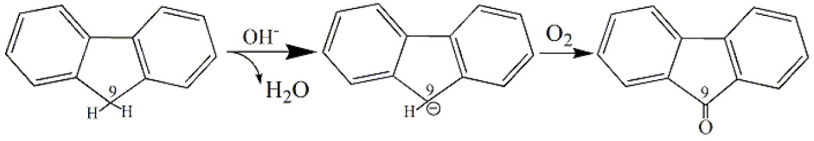
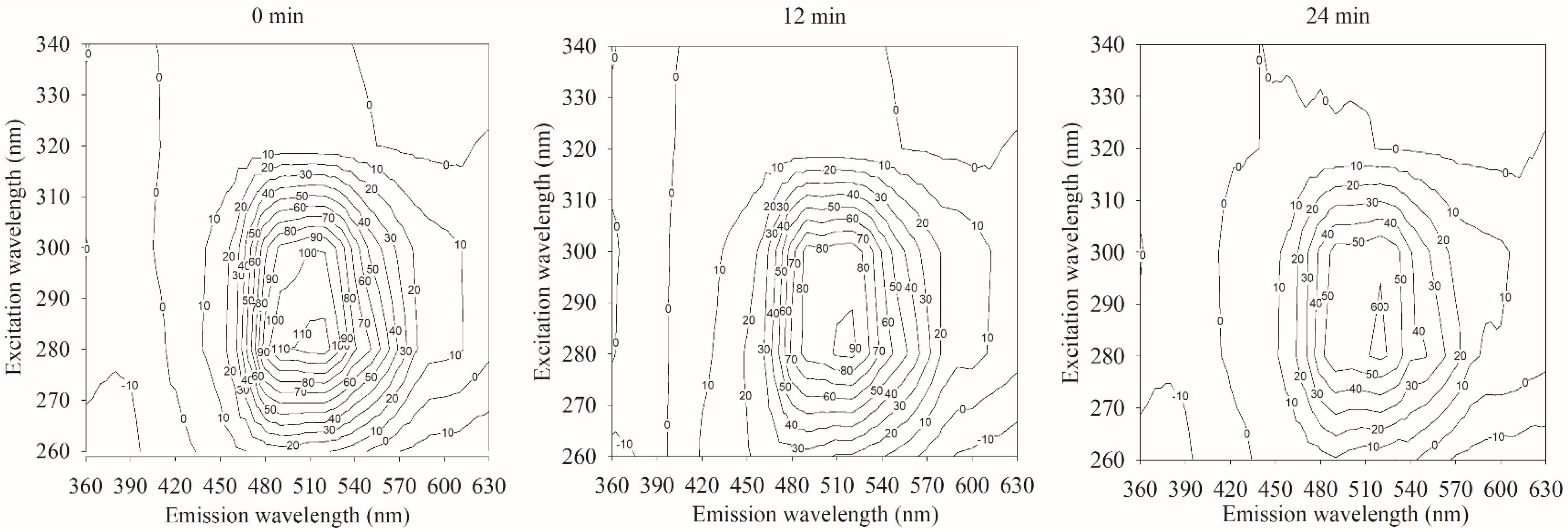
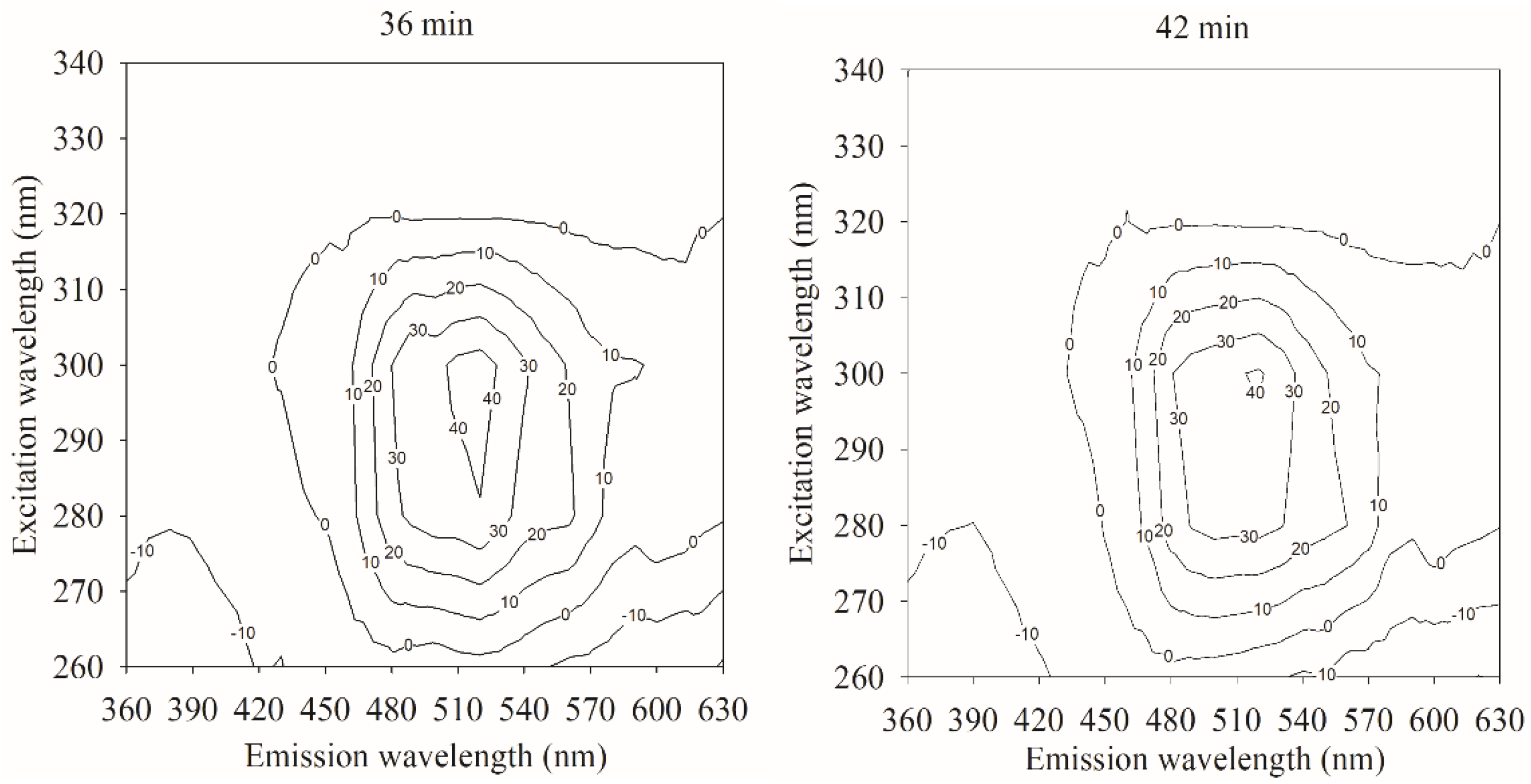
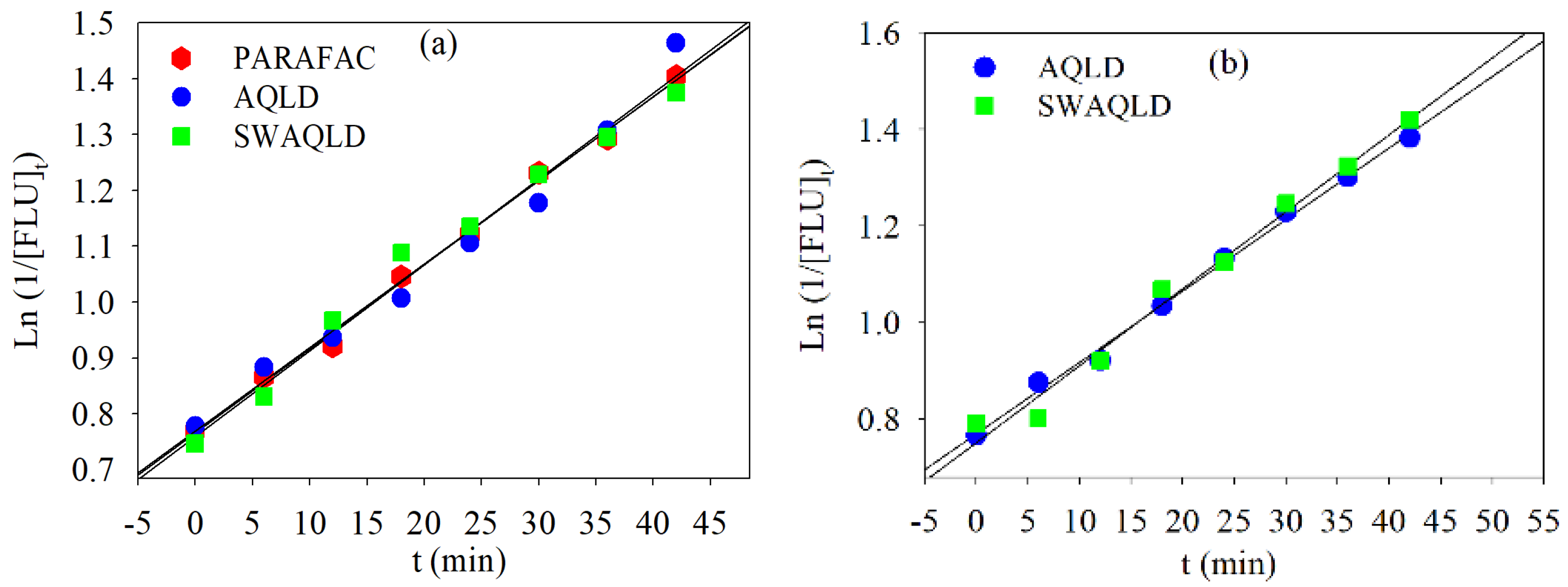
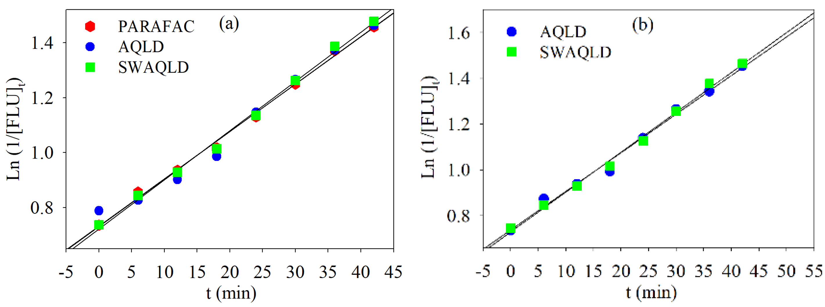
4.2.2. Global Analysis of the FLU Kinetic

FLU is a molecule that is quite stable but can nevertheless oxidize under alkaline conditions, as shown in Figure 1 [37]. In our experiments, the pH of mixed solutions is 10.6, and complete deoxygenation could not be achieved under heating conditions (40 °C), although Na2SO3 is added as a deoxygenator. Therefore, it could be deduced that FLU is very likely to be oxidized in the experimental condition. Figure 2 shows excitation–emission matrix phosphorescence (EEMP) plots of the calibration sample C4 with initial concentrations of 3.80 μg mL−1 of FLU, 0.8% acetonitrile–aqueous solvent, 0.6 mol L−1 KI, and 0.03 mol L−1 Na2SO3 acquired at five different times. It is, thus, easy to see that the intensity of the FLU phosphorescence gradually decreased with the duration of the reaction. The FLU phosphorescence decrease is very likely due to the oxidation of FLU to 9-fluorenone in water systems, and its product does not emit phosphorescence in the pH 10.6 mixed solution [38,39].

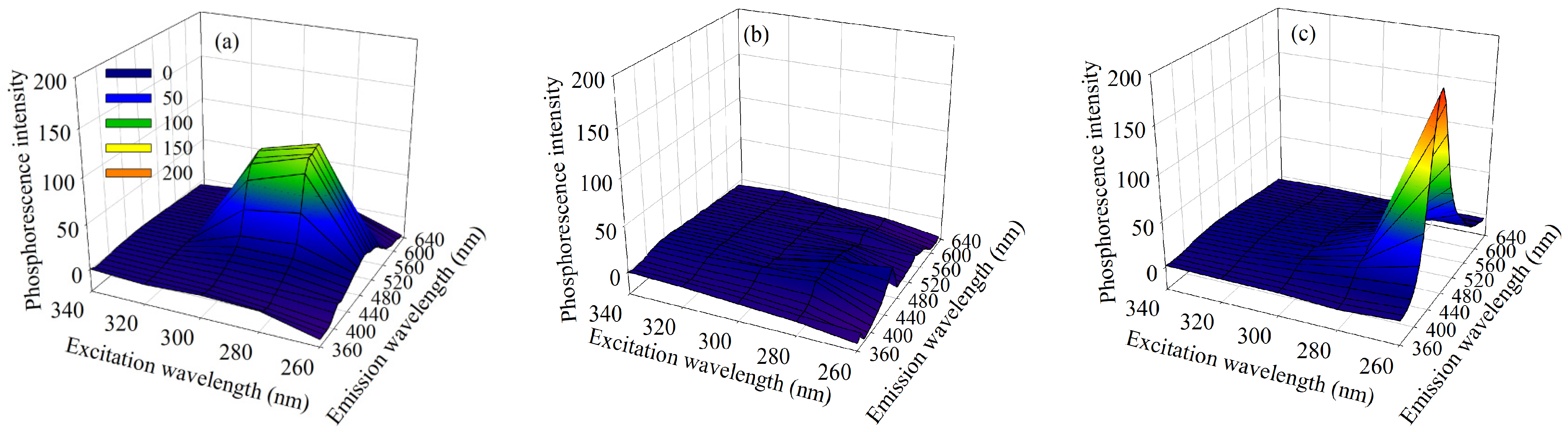
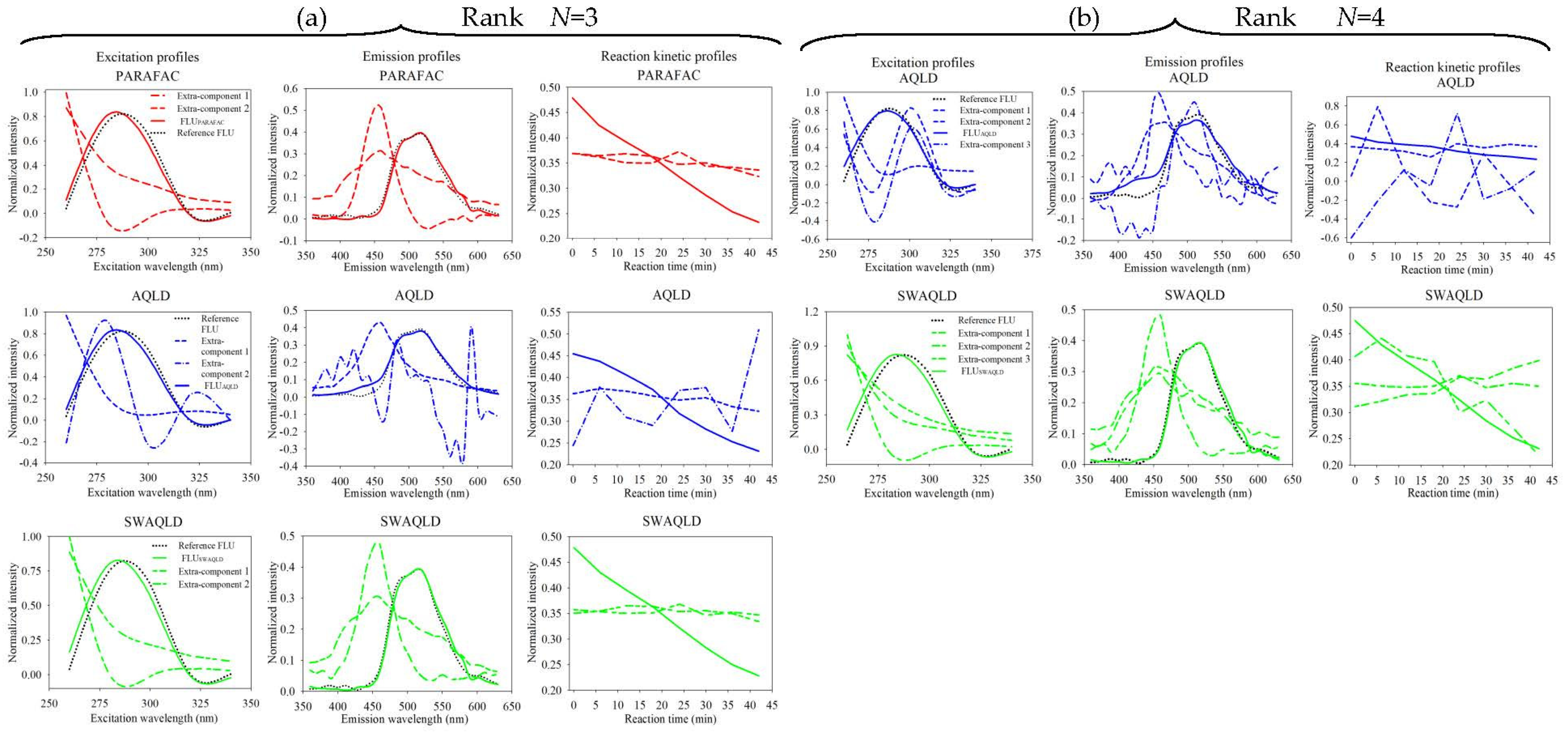
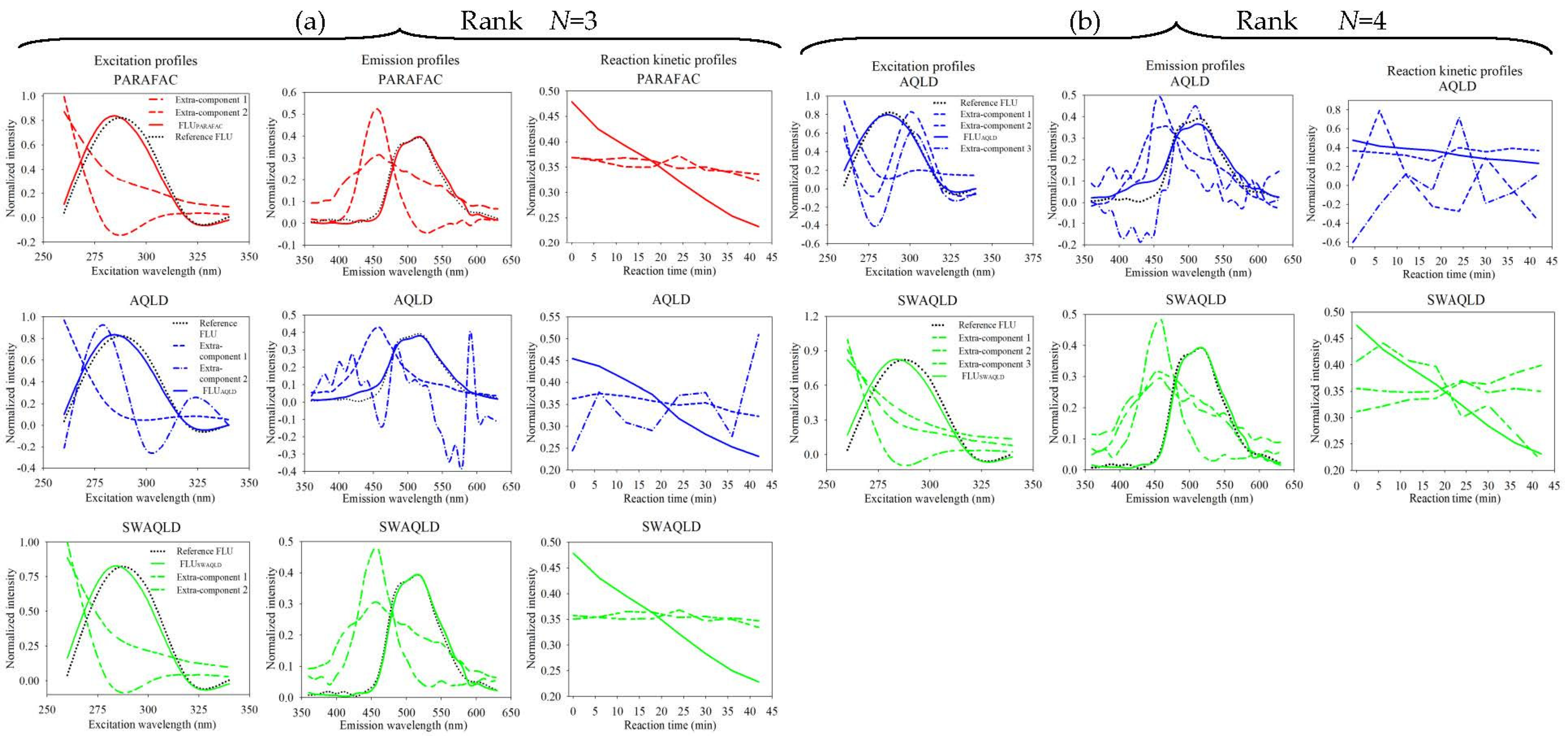
4.2.3. Spectral Characteristics of Samples

Figure 3a shows the three-dimensional phosphorescence spectrum of the calibration sample C4 at 0 min. The maximum excitation and emission wavelengths of fluorene are observed at 280 nm and 520 nm, respectively. Meanwhile, the EEMP spectra of a free-interference water sample and a wastewater one are also presented in Figure 3b,c, respectively. In the case of the free-interference water sample, it exhibits no significant spectral contribution. This is not the case for the wastewater sample, which has a strong emission peak, indicating that it likely contains inorganic or organic species that could interfere with the measurement of FLU in water systems. Therefore, it is clear that the free-interference water sample is a relatively simple case, but the wastewater one is undoubtedly very complex to manage, considering the quantification of FLU. What is more, it is impossible to directly study the oxidation kinetic process of phosphorescent FLU in the complex wastewater system with the ordinary phosphorescence method. It is in this sense that we demonstrate, in the following section, the potential of third-order multivariate calibration methods for the kinetic study of FLU, even in the presence of uncalibrated interfering species.

4.2.4. Analysis of FLU in Free-Interference Water Samples

The free-interference water samples were first used to evaluate the performance of our SWAQLD approach for the quantitative and kinetic study of FLU against the two classical approaches: PARAFAC and AQLD. Before decomposing the considered four-way phosphorescence data array with these three algorithms, the optimal number of components was estimated using CORCONDIA and AWQLD-MCS. The two methods applied to the considered data set, thus, allow us to select a potentially optimal number of factors equal to three (Supplementary Figure S2). Then, three-factor models were considered first in PARAFAC, AQLD, and SWAQLD, respectively. Figure 4a presents the resolved excitation, emission, and kinetic profiles of FLU in free-interference water samples extracted by the three methods. We can see that there are no significant differences among the extracted spectra representing FLU by these three methods, either at the excitation or emission levels when compared with the reference profile. Even if there was no ambiguity concerning the estimation of the number of components to be taken into account in the models for this rather simple chemical system, it seemed interesting to us to force these three methods to work with a higher rank in the scenario of four in order to estimate their robustness to this choice. Figure 4b presents again the resolved excitation, emission, and kinetic profiles of FLU in these new conditions for SWAQLD and AQLD methods. PARAFAC algorithm does not provide reliable and accurate resolved results (not shown here). These profiles are again quite consistent with the reference ones, which attests to a certain robustness for SWAQLD as well as AQLD in the analysis of relatively simple chemical systems. It is obvious that this chemical system without interference is not found in real water samples, but it allows for, nevertheless, a base of the analytical performance below which we cannot go. After observing the factorial decompositions proposed by these different methods, we can look at their exploitation from a quantitative point of view for the prediction of the FLU concentration of the six samples contained in the validation set. Statistical figures of merit obtained by the three methods are given in Table 1. A variable number of factors is also considered in these results in order to evaluate the robustness of the different approaches in this quantitative analysis framework. Thus, when we look at the averages of recovery for the different methods, we see fairly homogeneous values. However, SWAQLD gives better results (99.5 ± 4.2)% than those of PARAFAC ((101.9 ± 5.3)%) and AQLD ((101.3 ± 9.4)%) when N = 3. Concerning the root mean square error of prediction (RMSEP), it can be seen that the lowest and most stable values seem to be observed with the SWAQLD method, only 0.15 μg mL−1. However, we should not lose sight of the fact that these differences are very small. Therefore, it is difficult to say whether these three methods are statistically different when free-interference water samples are considered. Figure 4 also shows the oxidation kinetic profiles of FLU resolved (solid lines) by the three methods for the two considered ranks N = 3 and 4. As can be seen from the figure, the phosphorescence intensity of FLU decreases slowly and steadily, which is quite consistent. Considering that the FLU oxidation reaction follows a first-order kinetic model, its concentration follows the following equation as a function of time:
d [ F L U ] d t = K × [ F L U ]
In a trivial way, we then obtain the evolution of this concentration as a function of time, namely:
L n ( 1 [ F L U ] t ) = L n ( 1 [ F L U ] t = 0 ) + K t  
Figure 5 shows the plot of the natural logarithm of reciprocal of relative FLU concentration as a function of reaction time for PARAFAC, AQLD, and SWAQLD approaches. Generally speaking, we observe linear evolutions for the three methods when the rank is 3 (Figure 5a). It is much more interesting to see that this trend is still observed when the SWAQLD method as well as AQLD are used with an overestimated rank of 4 (Figure 5b).
However, PARAFAC does not provide acceptable results (not shown here). Table 6 presents the rate constants and the half-lives of the FLU oxidation obtained from experimental data presented in Figure 5. When the optimal rank of 3 is chosen, rate constants of the FLU oxidation are 0.0151, 0.0154, and 0.0150 min−1 for the three methods, respectively. Half-lives of FLU are 45.9, 45.0, and 46.2 min for the three methods, respectively. These values remain fairly stable for the SWAQLD and AQLD methods when the rank is overestimated, which are 0.0154 min−1 for rate constant and 45.2 min for half-life, on average. Although the experimental conditions can be considered simple with these free-interference water samples, we can see that the SWAQLD and AQLD methods are the most robust to the choice of rank both in terms of FLU quantification and estimation of kinetic parameters.

4.2.5. Analysis of FLU in Wastewater Samples

The objective of this section is to put the previous chemometric approaches into more complex situations by analyzing wastewater samples, which are naturally more complex matrices. It is particularly under these conditions that third-order multivariate calibration methods come into their own as they are potentially capable of quantifying species of interest in the presence of interferents that are not present during calibration. This is, of course, a situation that classical multivariate regression approaches cannot handle. As in the previous section, the PARAFAC, AQLD, and SWAQLD methods are applied for the number of factors equal to 3 and 4 on the wastewater samples, although the optimal number of components was three according to CORCONDIA and AWQLD-MCS (Supplementary Figure S3). Figure 6a presents the resolved excitation, emission, and kinetic profiles of FLU in wastewater samples extracted by the three methods for a rank equal to 3. It can, thus, be seen that all the profiles extracted by PARAFAC and SWAQLD for this specific rank are very similar. With regard to the AQLD method, a quite large deviation is observed between the FLU resolved emission spectrum and its reference in the 400–450 nm spectral range. Figure 6b shows the same set of profiles for AQLD and SWAQLD, but this time with a rank of 4. First of all, we can see that there is not an improvement under these new conditions for the FLU-resolved emission spectrum obtained from the AQLD method. One can even see that the differences are observed over an even wider spectral range. Regarding the SWAQLD method, we have a certain stability of the extracted excitation and emission profiles when the rank is overestimated. In addition, we have, indeed, a certain stability of the FLU kinetic profile for the SWAQLD method between the two rank values, which is not at all the case for the PARAFAC method (not shown here). We see in the next section the influence of these differences on the analytical performance of these chemometric methods.
As conducted previously, the profiles extracted by the three methods are used to quantify the FLU in the five wastewater samples contained in the validation set. Statistical figures of merit obtained by the three methods are given in Table 2. A variable number of factors is again considered. It should be noted that in addition to the RMSEP values, additional parameters have been estimated to further assess the analytical potential of the methods. Firstly, the sensitivity (SEN) of a model, related to the inverse of a regression line, thus makes it possible to estimate the influence that a small variation in the spectroscopic measurement could have on the concentration predictions. As for the detection limit (LOD), it will be estimated by multiplying by 3.3 the standard deviation of the FLU-predicted concentration in three blank samples. Finally, the limit of quantification (LOQ) will be estimated in the same way but using a multiplicative coefficient of 10. If we look at the RMSEP errors, we first note that the lowest values, 0.28 μg mL−1 for N = 3, are obtained for the SWAQLD method. This same method also shows a stability of this prediction error when faced with a change in rank, which is less the case for the AQLD one. This is due to the poor profile extracted in the previous section. We also observe that for a given method, the best sensitivity is always obtained for a rank of three. Obviously, this parameter is very sensitive to the change in model rank. Finally, with regard to the LOD and LOQ values, only the SWAQLD method proposes fairly stable values in the face of rank change. In view of all these observations, we can, therefore, say that the SWAQLD method is the most robust to the size of the models, which is an important advantage in an analytical implementation for the characterization of complex samples where interfering molecules are omnipresent.
Figure 7 shows the oxidation kinetic profiles of FLU resolved (solid lines) by the three methods for the two considered ranks N = 3 and 4. Although the set of points appears to be fairly aligned for all three methods with a rank of 3 (Figure 7a), there are some fairly significant differences from the results observed on the free-interference water samples (Figure 5a). Again, the PARAFAC method does not follow a linear relationship when a rank of 4 is selected (not shown here). Lastly, Table 7 gives the estimated kinetic parameters. We obtain in average a rate constant of approximately 0.017 min−1 and a half-life of 40.0 min. At first glance, it may seem surprising to find different values from those calculated for free-interference water samples. We must simply consider that inorganic or organic species present in the wastewater system potentially speed up the FLU oxidation reaction.

5. Conclusions

In the work, we developed a new third-order multivariate calibration method, named self-weighted alternating quadrilinear decomposition (SWAQLD), to deal with four-way phosphorescence data, which was obtained by recording the oxidation kinetic process of excitation–emission matrix phosphorescence (EEMP) signals of samples at the temperature of 40 °C using a fluorescence spectrophotometer for the first time. The newly developed method was applied for the quantification and kinetic study of fluorene in different water systems, such as free-interference water samples and wastewater samples, and compared with two classic methods, e.g., parallel factor analysis (PARAFAC) and alternating quadrilinear decomposition (AQLD). Through the analysis of simulated and real four-way data sets, we were able to show that the SWAQLD algorithm had good convergence properties and was less sensitive to noise and to overestimation of the number of factors than were the PARAFAC and AQLD methods. Furthermore, this was the first time applying the third-order multivariate calibration coupled with the EEMP technique to investigate the oxidation kinetic process of analytes, even in the presence of unseparated and uncalibrated interferents. The proposed analytical methodology will, therefore, be well-suited to the quantification and kinetic study of analytes of interest in a large number of complex environmental samples for which we will never be able to control, in advance, the presence or absence of certain chemical interferents.

Supplementary Materials

The following supporting information can be downloaded at: https://www.mdpi.com/article/10.3390/chemosensors11010053/s1, Figure S1: The results of 8 components for the simulated data with different homoscedastic noise levels using different methods, (a) CORCONDIA and (b) AWQLD-MCS. SMRC is the abbreviation of sorted mean relative concentration; Figure S2: The results of 8 components for the first real four-way phosphorescence data using different methods, (a) CORCONDIA and (b) AWQLD-MCS; Figure S3: The results of 8 components for the second real four-way phosphorescence data using different methods, (a) CORCONDIA and (b) AWQLD-MCS; Table S1: The convergence property of PARAFAC, AQLD and SWAQLD for simulated excitation-emission-kinetic four-way phosphorescence data with four levels of heteroscedastic noise; Table S2: The influence of heteroscedastic noise levels on correlation coefficients, root-mean-square errors of prediction (RMSEPs) and k values predicted by PARAFAC, AQLD and SWAQLD, respectively, for simulated four-way data; Table S3: The influence of factor numbers (N) on correlation coefficients, RMSEPs and k values predicted by PARAFAC, AQLD and SWAQLD, respectively, for simulated four-way data with ɑhomo = 2%; Table S4: The influence of factor numbers (N) on correlation coefficients, RMSEPs and k values predicted by PARAFAC, AQLD and SWAQLD, respectively, for simulated four-way data with ɑheter = 0.02%.

Author Contributions

X.-D.Q., conceptualization, methodology, and writing—original draft preparation; X.-H.Z., writing—review and editing and funding acquisition; R.A., investigation, validation, and data curation; J.Z., resources and funding acquisition; L.X., data curation and project administration; L.D., writing—review and editing and supervision. All authors have read and agreed to the published version of the manuscript.

Funding

This research was funded by the National Natural Science Foundation of China (Grant No. 32172300), the Research Foundation of Education Bureau of Hunan Province, China (Grant Nos. 21B0720, 22A0533), and Hunan provincial natural science foundation (Grant No. 2021JJ50151) for financial support. This research was also supported by the China Scholarship Council (Grant No. 202008430147) through the provision of financial support to visiting scholars participating in this study.

Institutional Review Board Statement

Not applicable.

Informed Consent Statement

Not applicable.

Data Availability Statement

Not applicable.

Acknowledgments

The authors would also like to thank the University of Lille for hosting Qing in the framework of this visit.

Conflicts of Interest

The authors declare no conflict of interest.

References

  1. Escandar, G.M.; Muñoz de la Peña, A. Multi-way calibration for the quantification of polycyclic aromatic hydrocarbons in samples of environmental impact. Microchem. J. 2021, 164, 106016. [Google Scholar] [CrossRef]
  2. Shang, F.K.; Wang, Y.T.; Wang, J.Z.; Zhang, L.; Cheng, P.F.; Wang, S.T. Determination of three polycyclic aromatic hydrocarbons in tea using four-way fluorescence data coupled with third-order calibration method. Microchem. J. 2019, 146, 957–964. [Google Scholar] [CrossRef]
  3. Sánchez-Barragán, I.; Costa-Fernández, J.M.; Pereiro, R.; Sanz-Medel, A.; Salinas, A.; Segura, A.; Fernández-Gutiérrez, A.; Ballesteros, A.; González, J.M. Molecularly imprinted polymers based on iodinated monomers for selective room-temperature phosphorescence optosensing of fluoranthene in water. Anal. Chem. 2005, 77, 7005–7011. [Google Scholar] [CrossRef]
  4. Chen, J.C.; Wu, H.L.; Wang, T.; Dong, M.Y.; Chen, Y.; Yu, R.Q. High-Performance Liquid Chromatography–Diode Array Detection Combined with Chemometrics for Simultaneous Quantitative Analysis of Five Active Constituents in a Chinese Medicine Formula Wen-Qing-Yin. Chemosensors 2022, 10, 238. [Google Scholar] [CrossRef]
  5. Baroudi, F.; Al-Alam, J.; Chimjarn, S.; Delhomme, O.; Fajloun, Z.; Millet, M. Conifers as environmental biomonitors: A multi-residue method for the concomitant quantification of pesticides, polycyclic aromatic hydrocarbons and polychlorinated biphenyls by LC-MS/MS and GC–MS/MS. Microchem. J. 2020, 154, 104593. [Google Scholar] [CrossRef]
  6. Araújo, A.S.; Castro, J.P.; Sperança, M.A.; Andrade, D.F.; de Mello, M.L.; Pereira-Filho, E.R. Multiway calibration strategies in laser-induced breakdown spectroscopy: A proposal. Anal. Chem. 2021, 93, 6291–6300. [Google Scholar] [CrossRef]
  7. Wu, H.L.; Wang, T.; Yu, R.Q. Recent advances in chemical multi-way calibration with second-order or higher-order advantages: Multilinear models, algorithms, related issues and applications. Trends Anal. Chem. 2020, 130, 115954. [Google Scholar] [CrossRef]
  8. Anzardi, M.B.; Arancibia, J.A.; Olivieri, A.C. Processing multi-way chromatographic data for analytical calibration, classification and discrimination: A successful marriage between separation science and chemometrics. Trends Anal. Chem. 2021, 134, 116128. [Google Scholar] [CrossRef]
  9. Pérez-Cova, M.; Jaumot, J.; Tauler, R. Untangling comprehensive two-dimensional liquid chromatography data sets using regions of interest and multivariate curve resolution approaches. Trends Anal. Chem. 2021, 137, 116207. [Google Scholar] [CrossRef]
  10. Mazivila, S.J.; Bortolato, S.A.; Olivieri, A.C. MVC3_GUI: A MATLAB graphical user interface for third-order multivariate calibration. An upgrade including new multi-way models. Chemom. Intel. Lab. Syst. 2018, 173, 21–29. [Google Scholar] [CrossRef]
  11. Yin, X.L.; Gu, H.W.; Liu, X.L.; Zhang, S.H.; Wu, H.L. Comparison of three-way and four-way calibration for the real-time quantitative analysis of drug hydrolysis in complex dynamic samples by excitation-emission matrix fluorescence. Spectrochim. Acta Part A 2018, 192, 437–445. [Google Scholar] [CrossRef] [PubMed]
  12. Osorio, A.; Toledo-Neira, C.; Bravo, M.A. Critical evaluation of third-order advantage with highly overlapped spectral signals. Determination of fluoroquinolones in fish-farming waters by fluorescence spectroscopy coupled to multivariate calibration. Talanta 2019, 204, 438–445. [Google Scholar] [CrossRef] [PubMed]
  13. Carabajal, M.D.; Arancibia, J.A.; Escandar, G.M. Excitation-emission fluorescence-kinetic third-order/four-way data: Determination of bisphenol A and nonylphenol in food-contact plastics. Talanta 2019, 197, 348–355. [Google Scholar] [CrossRef] [PubMed]
  14. Goicoechea, H.C.; Yu, S.; Moore, A.F.T.; Campiglia, A.D. Four-way modeling of 4.2K time-resolved excitation emission fluorescence data for the quantitation of polycyclic aromatic hydrocarbons in soil samples. Talanta 2012, 101, 330–336. [Google Scholar] [CrossRef] [PubMed]
  15. Lenardon Vinciguerra, L.; Carla Böck, F.; Pires Schneider, M.; Alejandra Pisoni Canedo Reis, N.; Flores Silva, L.; Christina Mendes de Souza, K.; Crivellaro Guerra, C.; de Araújo Gomes, A.; Maria Bergold, A.; Flôres Ferrão, M. Geographical origin authentication of southern Brazilian red wines by means of EEM-pH four-way data modelling coupled with one class classification approach. Food Chem. 2021, 362, 130087. [Google Scholar] [CrossRef]
  16. Fu, H.Y.; Wu, H.L.; Yu, Y.J.; Yu, L.L.; Zhang, S.R.; Nie, J.F.; Li, S.F.; Yu, R.Q. A new third-order calibration method with application for analysis of four-way data arrays. J. Chemom. 2011, 25, 408–429. [Google Scholar] [CrossRef]
  17. Cabrera-Bañegil, M.; Valdés-Sánchez, E.; Muñoz de la Peña, A.; Durán-Merás, I. Combination of fluorescence excitation emission matrices in polar and non-polar solvents to obtain three- and four-way arrays for classification of Tempranillo grapes according to maturation stage and hydric status. Talanta 2019, 199, 652–661. [Google Scholar] [CrossRef]
  18. Lozano, V.A.; Muñoz de la Peña, A.; Durán-Merás, I.; Espinosa Mansilla, A.; Escandar, G.M. Four-way multivariate calibration using ultra-fast high-performance liquid chromatography with fluorescence excitation–emission detection. Application to the direct analysis of chlorophylls a and b and pheophytins a and b in olive oils. Chemom. Intel. Lab. Syst. 2013, 125, 121–131. [Google Scholar] [CrossRef]
  19. Bailey, H.P.; Rutan, S.C. Comparison of chemometric methods for the screening of comprehensive two-dimensional liquid chromatographic analysis of wine. Anal. Chim. Acta 2013, 770, 18–28. [Google Scholar] [CrossRef]
  20. Arancibia, J.A.; Damiani, P.C.; Escandar, G.M.; Ibañez, G.A.; Olivieri, A.C. A review on second- and third-order multivariate calibration applied to chromatographic data. J.Chromatogr. B 2012, 910, 22–30. [Google Scholar] [CrossRef]
  21. Gao, Z.W.; Mou, L.; Xue, S.F.; Tao, Z.; Zeng, X. Cucurbit[8] urils-induced room temperature phosphorescence of phenanthrene and fluorene. Spectrosc. Spectral Anal. 2010, 30, 1026–1029. [Google Scholar] [CrossRef]
  22. Guo, J.; Yang, C.; Zhao, Y. Long-lived organic room-temperature phosphorescence from amorphous polymer systems. Accounts Chem. Res. 2022, 94, 5190–5195. [Google Scholar] [CrossRef] [PubMed]
  23. Arif, S.; Al-Tameemi, M.; Wilson, W.B.; Wise, S.A.; Barbosa, F.; Campiglia, A.D. Low-temperature time-resolved phosphorescence excitation emission matrices for the analysis of phenanthro-thiophenes in chromatographic fractions of complex environmental extracts. Talanta 2020, 212, 120805. [Google Scholar] [CrossRef] [PubMed]
  24. Pulgarin, J.A.M.; Molina, A.A.; Sanchez-Ferrer, I. Determination of propranolol and naproxen in urine by using excitation-emission matrix phosphorescence coupled with multivariate calibration algorithms. Curr. Pharm. Anal. 2012, 8, 83–92. [Google Scholar] [CrossRef]
  25. Muñoz de la Peña, A.; Mora Diez, N.; Bohoyo Gil, D.; Cano Carranza, E. Second-order data obtained by time-resolved room temperature phosphorescence. A new approach for PARAFAC multicomponent analysis. J. Fluoresc. 2009, 19, 345–352. [Google Scholar] [CrossRef]
  26. Arancibia, J.A.; Escandar, G.M. Room-temperature excitation–emission phosphorescence matrices and second-order multivariate calibration for the simultaneous determination of pyrene and benzo[a]pyrene. Anal. Chim. Acta 2007, 584, 287–294. [Google Scholar] [CrossRef]
  27. Arancibia, J.A.; Boschetti, C.E.; Olivieri, A.C.; Escandar, G.M. Screening of oil samples on the basis of excitation−emission room-temperature phosphorescence data and multiway chemometric techniques. Introducing the second-order advantage in a classification study. Anal. Chem. 2008, 80, 2789–2798. [Google Scholar] [CrossRef]
  28. Goicoechea, H.C.; Yu, S.; Olivieri, A.C.; Campiglia, A.D. Four-way data coupled to parallel factor model applied to environmental analysis:  Determination of 2,3,7,8-tetrachloro-dibenzo-para-dioxin in highly contaminated waters by solid−liquid extraction laser-excited time-resolved Shpol’skii spectroscopy. Anal. Chem. 2005, 77, 2608–2616. [Google Scholar] [CrossRef]
  29. Qing, X.D.; Wu, H.L.; Yan, X.F.; Li, Y.; Ouyang, L.Q.; Nie, C.C.; Yu, R.Q. Development of a novel alternating quadrilinear decomposition algorithm for the kinetic analysis of four-way room-temperature phosphorescence data. Chemom. Intel. Lab. Syst. 2014, 132, 8–17. [Google Scholar] [CrossRef]
  30. Harshman, R.A. Foundation of the PARAFAC procedure: Models and conditions for “explanatory” multimodal factor analysis. UCLA Work. Pap. Phon. 1970, 16, 1–84. Available online: https://www.psychology.uwo.ca/faculty/harshman/wpppfac0.pdf (accessed on 1 December 2022).
  31. Wu, H.L.; Shibukawa, M.; Oguma, K. An alternating trilinear decomposition algorithm with application to calibration of HPLC–DAD for simultaneous determination of overlapped chlorinated aromatic hydrocarbons. J. Chemom. 1998, 12, 1–26. [Google Scholar] [CrossRef]
  32. Chen, Z.P.; Wu, H.L.; Jiang, J.H.; Li, Y.; Yu, R.Q. A novel trilinear decomposition algorithm for second-order linear calibration. Chemom. Intel. Lab. Syst. 2000, 52, 75–86. [Google Scholar] [CrossRef]
  33. Bro, R.; Kiers, H.A.L. A new efficient method for determining the number of components in PARAFAC models. J. Chemom. 2003, 17, 274–286. [Google Scholar] [CrossRef]
  34. Qing, X.D.; Li, Y.; Wen, J.; Shen, X.Z.; Li, C.Y.; Liu, X.L.; Xie, J. A new method to determine the number of chemical components of four-way data from mixtures. Microchem. J. 2017, 135, 114–121. [Google Scholar] [CrossRef]
  35. Wang, X.M.; Dong, M.J.; Li, Z.J.; Wang, Z.P.; Liang, F.S. Recent advances of room temperature phosphorescence and long persistent luminescence by doping system of purely organic molecules. Dyes Pigments 2022, 204, 2–12. [Google Scholar] [CrossRef]
  36. Machicote, R.G.; Bruzzone, L. Simultaneous determination of carbaryl and 1-naphthol by first-derivative synchronous non-protected room temperature phosphorescence. Anal. Sci. 2009, 25, 623–626. [Google Scholar] [CrossRef] [Green Version]
  37. Liu, L.L.; Yang, B.; Zhang, H.Y.; Tang, S.; Xie, Z.Q.; Wang, H.P.; Wang, Z.M.; Lu, P.; Ma, Y.G. Role of Tetrakis(triphenylphosphine)palladium(0) in the degradation and optical properties of fluorene-based compounds. J. Phys. Chem. C 2008, 112, 10273–10278. [Google Scholar] [CrossRef]
  38. Wang, Y.S.; Yang, J.; Tian, Y.; Fang, M.M.; Liao, Q.Y.; Wang, L.W.; Hu, W.P.; Tang, B.Z.; Li, Z. Persistent organic room temperature phosphorescence: What is the role of molecular dimers? Chem. Sci. 2020, 11, 833–838. [Google Scholar] [CrossRef] [Green Version]
  39. Liu, L.L.; Tang, S.; Liu, M.R.; Xie, Z.Q.; Zhang, W.; Lu, P.; Hanif, M.; Ma, Y.G. Photodegradation of polyfluorene and fluorene oligomers with alkyl and aromatic disubstitutions. J. Phys. Chem. B 2006, 110, 13734–13740. [Google Scholar] [CrossRef]
Figure 1. The oxidation pathway of FLU.
Chemosensors 11 00053 g001
Figure 2. The kinetic evolution contour plots of excitation–emission matrix phosphorescence for calibration sample C4 at specific times (0, 12, 24, 36, and 42 min).
Chemosensors 11 00053 g002aChemosensors 11 00053 g002b
Figure 3. Excitation–emission matrix phosphorescence corresponding to samples of (a) a 3.80 μg mL−1 FLU sample, (b) a free-interference water sample, and (c) a wastewater one.
Chemosensors 11 00053 g003
Figure 4. Resolved excitation, emission, and kinetic profiles, normalized to unit length obtained from PARAFAC, AQLD, and SWAQLD for the analysis of four-way phosphorescence data of free-interference water samples with a rank N = 3 (a) or 4 (b). The black dotted lines denote the FLU reference profiles. The red, blue, and green solid lines represent the FLU-resolved profiles obtained from PARAFAC, AQLD, and SWAQLD, respectively. Other extracted profiles represent additional extracted components.
Chemosensors 11 00053 g004
Figure 5. The plot of the natural logarithm of reciprocal of relative concentration (Ln(1/[FLU]t)) versus time (t) for PARAFAC, AQLD, and SWAQLD in the case of free-interference water samples and a rank of 3 (a) or 4 (b).
Chemosensors 11 00053 g005
Figure 6. Resolved excitation, emission, and kinetic profiles, normalized to unit length obtained from PARAFAC, AQLD and SWAQLD for the analysis of four-way phosphorescence data of wastewater samples with a rank N = 3 (a) or 4 (b). The black dotted lines denote the FLU reference profiles. The red, blue, and green solid lines represent the FLU-resolved profiles obtained from PARAFAC, AQLD, and SWAQLD, respectively. Other extracted profiles represent additional extracted components.
Chemosensors 11 00053 g006
Figure 7. The plot of the natural logarithm of reciprocal of relative concentration (Ln(1/[FLU]t)) versus time (t) for PARAFAC, AQLD, and SWAQLD in the case of wastewater samples and a rank of 3 (a) or 4 (b).
Chemosensors 11 00053 g007
Table 1. Statistical figures of merit concerning the fluorene quantification in free-interference water samples by using third-order calibration methods (PARAFAC, AQLD, and SWAQLD) with different rank values.
Sample
No.
Reference Concentration
(μg.mL−1)
Recovery (%)
PARAFACAQLDSWAQLD
N = 3N = 3N = 4N = 3N = 4
V011.71117.8117.3115.8111.2113.2
V022.09101.891.393.695.596.3
V032.4797.788.589.696.696.2
V042.85100.4102.1100.499.5101.7
V053.23100.0112.7111.4100.4105.6
V063.6194.195.998.693.697.3
AR a (%)
SDR b (%)
101.9
5.3
101.3
9.4
101.6
8.0
99.5
4.2
101.7
5.1
RMSEP c (μg.mL−1)0.170.280.240.150.15
a AR: average recovery. b SDR: standard deviation of recovery. c Root mean square error of prediction (RMSEP) is calculated by RMSEP = [ 1 I 1 ( c ref c pred ) 2 ] 1 / 2 , where cref and cpred are the reference and predicted values, respectively.
Table 2. Statistical figures of merit concerning the fluorene quantification in wastewater samples by using third-order calibration methods (PARAFAC, AQLD, and SWAQLD) with different rank values.
Sample
No.
Reference Concentration
(μg mL−1)
Recovery (%)
PARAFACAQLDSWAQLD
N = 3N = 3N = 4N = 3N = 4
W012.09121.4122.7108.1113.6118.8
W022.4786.591.797.892.993.9
W032.8593.896.984.892.894.6
W043.2389.594.984.190.088.4
W053.61103.0105.591.693.697.3
AR98.8102.393.396.698.6
SDR10.79.47.76.88.1
RMSEP (μg mL−1)0.340.290.380.280.30
SEN (mL μg−1) a12.9841.338.0318.711.98
LOD (μg mL−1) b0.210.130.040.100.11
LOQ (μg mL−1) c0.640.400.110.290.34
a SEN: sensitivity. b LOD: limit of detection = 3.3σ0, where σ0 is the standard deviation of the FLU-predicted concentration in three blank samples. c LOQ: limit of quantification = 10σ0.
Table 3. The convergence property of PARAFAC, AQLD, and SWAQLD for simulated excitation–emission–kinetic four-way phosphorescence data with four levels of homoscedastic noise.
Noisehomo (%)Iteration Number (Computation Time (s))
PARAFACAQLDSWAQLD
MinMaxAverage aMinMaxAverageMinMaxAverage
0.02 162 (250.9)1951 (2756.9)281
(443.8)
5
(0.4)
10
(1.0)
6
(0.6)
52
(4.3)
183
(13.3)
80
(6.6)
0.2 118 (191.4)1921 (3113.2)235
(375.9)
5
(0.4)
10
(0.9)
6
(0.6)
24
(1.8)
168
(11.6)
66
(4.6)
2135 (165.7)2132 (4230.5)756 (1156.6)5
(0.4)
13
(1.1)
7
(0.7)
29
(1.8)
227
(16.0)
58
(3.9)
20 91
(123.1)
882 (1473.3)252
(412.6)
8
(0.8)
68
(5.0)
13
(1.1)
29
(2.0)
256
(15.4)
47
(3.1)
a These values are average results for 100 runs with random initialization.
Table 4. The influence of homoscedastic noise levels (ɑhomo) on correlation coefficients, RMSEPs, and k values predicted by PARAFAC, AQLD, and SWAQLD, respectively, for simulated four-way data.
Mode PARAFACAQLDSWAQLD
0.02%0.2%2%20%0.02%0.2%2%20%0.02%0.2%2%20%
Aa11.000 a1.00001.00000.99981.00001.00001.00000.99881.00001.00001.00000.9997
a21.00001.00001.00000.99991.00001.00001.00000.99981.00001.00001.00000.9998
a31.00001.00001.00000.99981.00001.00001.00000.99761.00001.00001.00000.9998
Bb11.00001.00001.00000.99941.00001.00001.00000.99861.00001.00001.00000.9994
b21.00001.00001.00000.99991.00001.00001.00000.99841.00001.00001.00000.9999
b31.00001.00001.00000.99991.00001.00001.00000.99521.00001.00001.00000.9999
Cc11.00001.00001.00001.00001.00001.00001.00000.99911.00001.00001.00000.9997
c21.00001.00001.00001.00001.00001.00001.00000.99971.00001.00001.00000.9999
c31.00001.00001.00001.00001.00001.00001.00000.99961.00001.00001.00000.9997
Dd11.00001.00001.00001.00001.00001.00001.00000.99201.00001.00001.00000.9999
d21.00001.00001.00001.00001.00001.00001.00000.99971.00001.00001.00001.0000
d31.00001.00001.00000.99991.00001.00001.00000.99021.00001.00001.00001.0000
RMSEPAnalyte 10.00000.00020.00050.00260.00000.00010.00070.0546 c0.00000.00030.00060.0049
Analyte 20.00000.00010.00060.00320.00000.00010.00100.00930.00000.00020.00030.0023
Predicted k b0.09990.09920.10050.09410.09990.09960.09400.03670.09990.09920.10000.0997
a All values in the first 12 rows of this table correspond to the correlation coefficient between the profiles predicted by the different methods and the reference profiles. b The chosen constant rate of the analyte in the simulated data set is 0.1000. c Bold characters are used to highlights the worst results.
Table 5. The influence of factor numbers (N) on correlation coefficients, RMSEPs, and k values predicted by PARAFAC, AQLD, and SWAQLD, respectively, for simulated four-way data with ɑhomo = 0.02%.
ModePARAFACAQLDSWAQLD
N = 3N = 4N = 10N = 3N = 4N = 10N = 3N = 4N = 10
Aa11.00001.00000.99641.00001.00001.00001.00001.00001.0000
a21.00001.00000.99991.00001.00001.00001.00001.00001.0000
a31.00001.00000.99191.00001.00001.00001.00001.00001.0000
Bb11.00001.00000.91221.00001.00001.00001.00001.00001.0000
b21.00001.00000.96381.00001.00001.00001.00001.00001.0000
b31.00001.00000.93971.00001.00001.00001.00001.00001.0000
Cc11.00001.00001.00001.00001.00001.00001.00001.00001.0000
c21.00001.00000.99951.00001.00001.00001.00001.00001.0000
c31.00001.00000.98131.00001.00001.00001.00001.00001.0000
Dd11.00001.00000.98911.00001.00001.00001.00001.00001.0000
d21.00001.00000.91961.00001.00001.00001.00001.00001.0000
d31.00001.00000.99671.00001.00001.00001.00001.00001.0000
RMSEPAnalyte 10.00000.00000.06790.00000.00000.00000.00000.00000.0001
Analyte 20.00000.00140.24550.00000.00000.00000.00000.00000.0000
Predicted k0.09990.10000.06400.09990.09990.10000.09990.10000.1001
Table 6. Evaluation of the FLU rate constant considering different approaches and ranks.
Regression
Equation
Correlation
Coefficient
Rate Constant
(min−1)
Half Life
(min)
PARAFAC (N = 3)y = 0.0151x + 0.76550.99620.015145.9
AQLD (N = 3)y = 0.0154x + 0.76000.98890.015445.0
AQLD (N = 4)y = 0.0148x + 0.76980.99800.014846.8
SWAQLD (N = 3)y = 0.0150x + 0.76870.99280.015046.2
SWAQLD (N = 4)y = 0.0159x + 0.75260.99310.015943.6
Table 7. Regression equation, correlation coefficient, rate constant, and half-life of the oxidation reaction of FLU in wastewater samples.
Regression
Equation
Correlation
Coefficient
Rate Constant
(min−1)
Half Life
(min)
PARAFAC (N = 3)y = 0.0172x + 0.73210.99810.017240.3
AQLD (N = 3)y = 0.0173x + 0.73100.99080.017340.1
AQLD (N = 4)y = 0.0169x + 0.73740.99540.016941.0
SWAQLD (N = 3)y = 0.0179x + 0.72190.99780.017938.7
SWAQLD (N = 4)y = 0.0174x + 0.72880.99770.017439.8
Disclaimer/Publisher’s Note: The statements, opinions and data contained in all publications are solely those of the individual author(s) and contributor(s) and not of MDPI and/or the editor(s). MDPI and/or the editor(s) disclaim responsibility for any injury to people or property resulting from any ideas, methods, instructions or products referred to in the content.

