Elemental Determination in Stainless Steel via Laser-Induced Breakdown Spectroscopy and Back-Propagation Artificial Intelligence Network with Spectral Pre-Processing

Abstract

Minor elements significantly influence the properties of stainless steel. In this study, a laser-induced breakdown spectroscopy (LIBS) technique combined with a back-propagation artificial intelligence network (BP-ANN) was used to detect nickel (Ni), chromium (Cr), and titanium (Ti) in stainless steel. For data pre-processing, cubic spline interpolation and wavelet threshold transform algorithms were used to perform baseline removal and denoising. The results show that this set of pre-processing methods can effectively improve the signal-to-noise ratio, remove the baseline of spectral baseline, reduce the average relative error, and reduce relative standard deviation of BP-ANN predictions. It indicates that BP-ANN combined with pre-processing methods has promising applications for the determination of Ni, Cr, and Ti in stainless steel with LIBS and improves prediction accuracy and stability.

1. Introduction

Laser-induced breakdown spectroscopy (LIBS) is a popular atomic emission spectroscopy technology that uses a high-energy laser pulse to form plasma [1]. Furthermore, the composition and concentrations of elements in a sample can be determined by analyzing the emission spectrum. LIBS first appeared in the 1960s and was first proposed by Brech et al. [2]. LIBS exhibits the advantages of no pre-processing, such as less damage to samples, suitability for various forms of samples, and remote and real-time online detection [3]. LIBS technology has wide applications in environmental geology [4,5], military [6], materials [7], metallurgy [8], biology [9,10], archaeology [11], environmental monitoring [12], and other fields. Owing to spectral noise, baseline drift, self-absorption, and other phenomena, there is a large amount of interference information in the LIBS spectrum, which makes quantitative analysis difficult [13]. Furthermore, for the widely used internal standardization method, it is difficult to know the internal standard of steel in practical applications [14]. Multivariate methods [15] are available to avoid this problem, which uses standard samples to train a model and to predict the test sample [16]. An artificial neural network (ANN) is a popular multivariate calibration tool [17] and a widely used machine learning model with a strong input–output nonlinear mapping ability [18]. ANN can identify nonlinear features and screen interference information, which further expands the prospect of LIBS technology [19]. At present, the most commonly used ANN scheme in LIBS research is back-propagation artificial neural network (BP-ANN) [17]. Some examples of quantitative analysis based on BP-ANN in LIBS technology are given in

Table 1. Examples of quantitative analysis based on BP-ANN in LIBS technology.

Year	Author	Sample	Brief Introduction
2006	Sirven et al. [20]	soil samples	Cr concentration in soil samples was quantitatively analyzed. By comparing the prediction accuracy and the detection limit of BP-ANN, PLSR and the standard calibration curve, the superiority of BP-ANN in LIBS analysis is proved.
2008	Motto-Ros et al. [21]	natural rock and soil samples	Simultaneous measurement of multiple element concentrations has been demonstrated and is of great significance in planetary science.
2009	Inakollu et al. [22]	Al alloy samples	The measurement results of artificial neural networks with the traditional one-way calibration method were compared, and it was determined that in most cases, BP-ANN exhibits better measurement performance and accuracy.
2010	Rezaei et al. [19]	aluminum standards	The effect of self-absorption on concentration prediction of the aluminum standard samples via two approaches—calibration curve and ANN—in the LIBS experiment is studied.
2014	D’Andrea et al. [23]	bronze alloys samples	Forward feature selection has been adopted to reduce the number of input variables to the neural network to the minimum number of variables, providing a viable, fast, and robust method for LIBS quantitative analysis.
2017	Moncayo et al. [24]	milk samples	The results demonstrate that LIBS/BP-ANN combination, supported by its speed of analysis, reduced cost, and ease of use, has the potential to serve as a useful screening tool in the quality control of milk.
2017	Hu et al. [3]	geological standard samples from USGS	The concentration of iron in the concentrations of BCR-1G, BHVO-2G, BIR-1G, GSD-1G, and GSE-1G was determined, and the relative error of the results is less than 6%.
2020	Yang et al. [25]	vegetables samples	Combined with the advantages of reducing the multiple collinearities of PLS independent variables and the nonlinear processing ability of ANN, the accuracy of LIBS quantitative analysis is significantly improved.

.

As a black box system, ANN establishes complicated input–output correlations [26]. Hence, we should ensure that the characteristic information of determining elements is provided to the ANN model. By using the chemometrics method for data pre-processing, the influence of a variety of non-target factors can be reduced [27]. Now, the commonly used spectral pre-processing includes baseline calibration and spectral noise reduction. The target baseline point selection method based on the inter-partition extreme value is one of the commonly used methods in the segmented fitting baseline correction [28,29]. In 2009, Sun et al. [30] presented a method of background correction based on linear interpolation. Tan et al. [31] used the spline interpolation method to remove the baseline in LIBS, which shows that the spline interpolation method can effectively detect and correct the continuous background. In addition, for filtering noise near the characteristic peaks, the wavelet transform is a common method. Wavelet transform has the advantages of simplicity and reconfigurability, which can improve the study of time-frequency domain characteristics [32]. Yuan et al. [33] used wavelet transform and least squares to build a hybrid model and applied wavelet analysis algorithms to the background removal of LIBS spectra for the first time. Zhang et al. [32] used correlation analysis to optimize the wavelet noise threshold in a way that improved the signal-to-noise ratio and the fitted correlation coefficient of the internal calibration curve while reducing the detection limit.

Stainless steel is an important material with a wide range of applications in daily life and the industry. The types and contents of the minor elements in stainless steel determine its properties [34,35]. Therefore, it is of great significance to the manufacturing industry to determine these elements for the evaluation of stainless steel properties. In recent years, LIBS has been used in steel analysis and industry applications [36]. Li et al. [37] used LIBS with laser-induced fluorescence and realized the sensitive determination of trace chromium in low-alloy steels, and the performance of quantitative analysis is given by the standard calibration curve (LoD of 8.64 μg g⁻¹, R² of 0.992, ARSD of 2.89%). Zhang et al. [38] demonstrated LIBS with laser-induced molecular fluorescence as a capable and potential approach for quickly determining the silicon element in steel industries. Cui et al. [39] successfully measured the trace carbon in steel by long-short double-pulse LIBS, and the relative error of prediction (REP) was between 6.1% and 35.7% and the relative standard deviation (RSD) was between 13.9% and 58.3% for five measured samples.

To improve the quantitative accuracy analysis of stainless steel samples using LIBS, a series of data pre-processing methods were proposed. Cubic spline interpolation and wavelet threshold transform algorithms were used to correct the baseline and filter the noise in the LIBS spectral data, respectively. We then selected the characteristic spectral lines with the Pearson correlation coefficient between the strength of the characteristic spectral lines and element content. Finally, we used the BP-ANN model to predict the elemental content of Ni, Cr, and Ti in stainless steel.

2. Experiments and Methods

2.1. Experiments

As shown in Figure 1, a lamp pumping pulse Q-switch laser (Penny-300-TH) was used in the experiment with a pulse wavelength of 1064 nm, a single pulse energy of about 35 mJ, a pulse duration of 8.4 ns, and a spot size of the beam of about 100 μm. Three mirrors were used to reflect the pulse and to adjust the optical path; the pulse was then focused on the sample surface via a focusing lens. The sample was placed on a three-dimensional mobile platform, whereby its surface relative to the laser focused point can be controlled. A spectrometer (Andor Technology Ltd., Belfast, UK, SR-750-B1) was used to collect the plasma spectrum using a probe. At the front of the probe is a collimating lens with a focal length of 100 mm, through which the light is spatially integrated to an optical fiber 100 mm away from the lens; then, the optical fiber transmits the light to the spectrometer. In addition, the spectrum signal was converted and transmitted to a computer using an ICCD (Andor Technology Ltd., iStar 334T). For the spectrometer, a delay time of 6 μs, a gate width of 15 μs, and a grating of 1200 gr/mm corresponding to a resolution of 0.04 nm were set. Please note that the delay time here is the acquisition delay set by the software, and the actual delay was smaller than 6 μs. During the experiment, the laser power supply, laser, and ICCD were controlled using a delay generator (DG645). We also set up a certain acquisition delay using the delay generator, such that the spectrometer accumulates 3 pulses for a spectrum and obtains an average, and better spectral signal.

Seven standard stainless steel samples were used for spectral analysis (GBW 01659a, GBW 01660a, GBW 01661a, GBW 01662a, GBW 01663a, GBW 01664a, and GBW 01665a) purchased from NCS Testing Technology Co., Ltd., Beijing, China.

Table 2. Reference content of Ni, Cr, and Ti in the samples (wt%).

Sample	Ni	Cr	Ti
GBW 01659a	4.76	28.00	0.053
GBW 01660a	14.58	14.37	0.475
GBW 01661a	19.13	10.66	0.577
GBW 01662a	11.24	19.73	0.253
GBW 01663a	22.77	7.65	0.774
GBW 01664a	7.34	24.40	0.170
GBW 01665a	8.72	17.57	0.336

shows composition of the employed samples. Each sample is repeatedly collected for 10 times, and there are 70 spectral data in total.

2.2. Methods of LIBS Element Content Calibration

It is well known that the LIBS spectrum characteristic line intensity can be indicated as a function [40]:

$$I=F\frac{A_{ij}{g}_i}{U_n\left(T\right)} C_n{e}^{-E/kT}$$

(1)

where $I$ denotes the characteristic line intensity of species n; $F$ is the experimental parameter affected by the efficiency of the optical system and plasma; $i$ and $j$ are the high-energy and low-energy level transitions, respectively; $A_{ij}$ is the transition probability; $g_i$ is the statistical weight of the high-energy level; $U_n\left(T\right)$ is the partition function at temperature $i$; $C_n$ is the content of element n; $E$ is the excitation energy of the transition; and $K$ is the Boltzmann constant.

Therefore, a linear relationship between characteristic line intensity and element content was established theoretically when a plasma is in a state of local thermodynamic equilibrium. Usually, an element corresponds to multiple characteristic spectral lines and the relationship is approximately as follows [40]:

$$C_n={\displaystyle \sum }\left(w_k·I_k\right)+b_0$$

(2)

where $w_k$ denotes the correlation coefficient and $I_k$ denotes the intensity of the characteristic line. However, in practice, the relationship between spectral line intensity and element concentration is nonlinear. There are obvious difficulties in measuring the element concentrations using traditional internal calibration. A back-propagation artificial neural network (BP-ANN) exhibits a good ability to handle nonlinear data. We decided to use BP-ANN to handle the spectral data of this experiment.

2.3. BP-ANN and Quantitative Analysis

The back-propagation artificial neural network is composed of multiple layers, including the input, hidden, and output layers, with each layer containing multiple nodes. The nodes between the previous and subsequent layers are connected to each other. There are forward propagation processes and back-propagation processes in BP-ANN learning. In the forward propagation process, each node accepts the node of the previous layer as the input and outputs the results to the next layer through the activation function. As shown in Figure 2, the propagation equation is [41]:

$$y_j=f_1\left({\displaystyle \sum }{w}_{ij}{x}_i-{\theta }_i\right)$$

(3)

$$z_h=f_2\left({\displaystyle \sum }{w}_{hj}{y}_i\right)$$

(4)

where $x_i$ denotes the input value; $y_i$ denotes the output value of the hidden layer with weight $w_{ij}$; ${\theta }_i$ denotes the threshold for neuron i of the hidden layer; $z_h$ denotes the output of the output layer; and $f_1$ and $f_2$ denote the activation and transfer functions of the hidden and output layers, respectively. The functions are set as follows:

$$f_1\left(x\right)=\mathit{max}\left(0,x\right)$$

(5)

$$f_2\left(x\right)=wx+b$$

(6)

The back-propagation process is the reverse transfer of the output error and corrects the weight of each node using the gradient descent method to minimize the error signal [42].

In this study, the BP-ANN model built on Keras and the mean square error were used as the loss functions. The number of nodes in the input, hidden, and output layers are 50, 50 and 1, respectively. The number of iterations was set to 600. These parameters were obtained by comparing them in several tests. Other adjustable coefficients are the default settings.

2.4. Data Pre-Processing Methods

Owing to the influence of environmental noise and other factors, continuous background noise is present in the spectrum, which results in a high baseline of the spectrum. To obtain more accurate spectral line information, we used a cubic spline interpolation algorithm for the baseline calibration and noise reduction. Cubic spline interpolation can smoothly fit discrete data and has been widely used in many applications including graphics processing, data fitting, and computer design, etc. In cubic spline interpolation for the data set with $m+1$ given points, a cubic spline is constructed between the data points by using an $m$ cubic polynomial [43]. In this study, the cubic splines with a natural boundary condition was used.

To further remove noise, we used the wavelet threshold transform algorithm. Wavelet threshold transform is a good and convenient method for noise reduction and data decorrelation, and it is based on orthogonal wavelet transform [44]. The general process is wavelet decomposition, threshold selection, and wavelet reconstruction of the signal after filtering [45]. In discrete wavelet transform (DWT), the wavelet function is defined as [46]:

$${\mathsf{\Psi }}_{m,n}\left(\mathit{t}\right)=a^{-m/2}\mathsf{\Psi }\left({\mathit{a}}^{-m}t-nb\right)$$

(7)

where $a$ and $b$ influence the dilation and translation parameters, $(a>1, b\in R, m\in Z, n\in Z)$. In this study, following general practice, $a$ and $b$ were set to 2 and 1, respectively.

3. Results

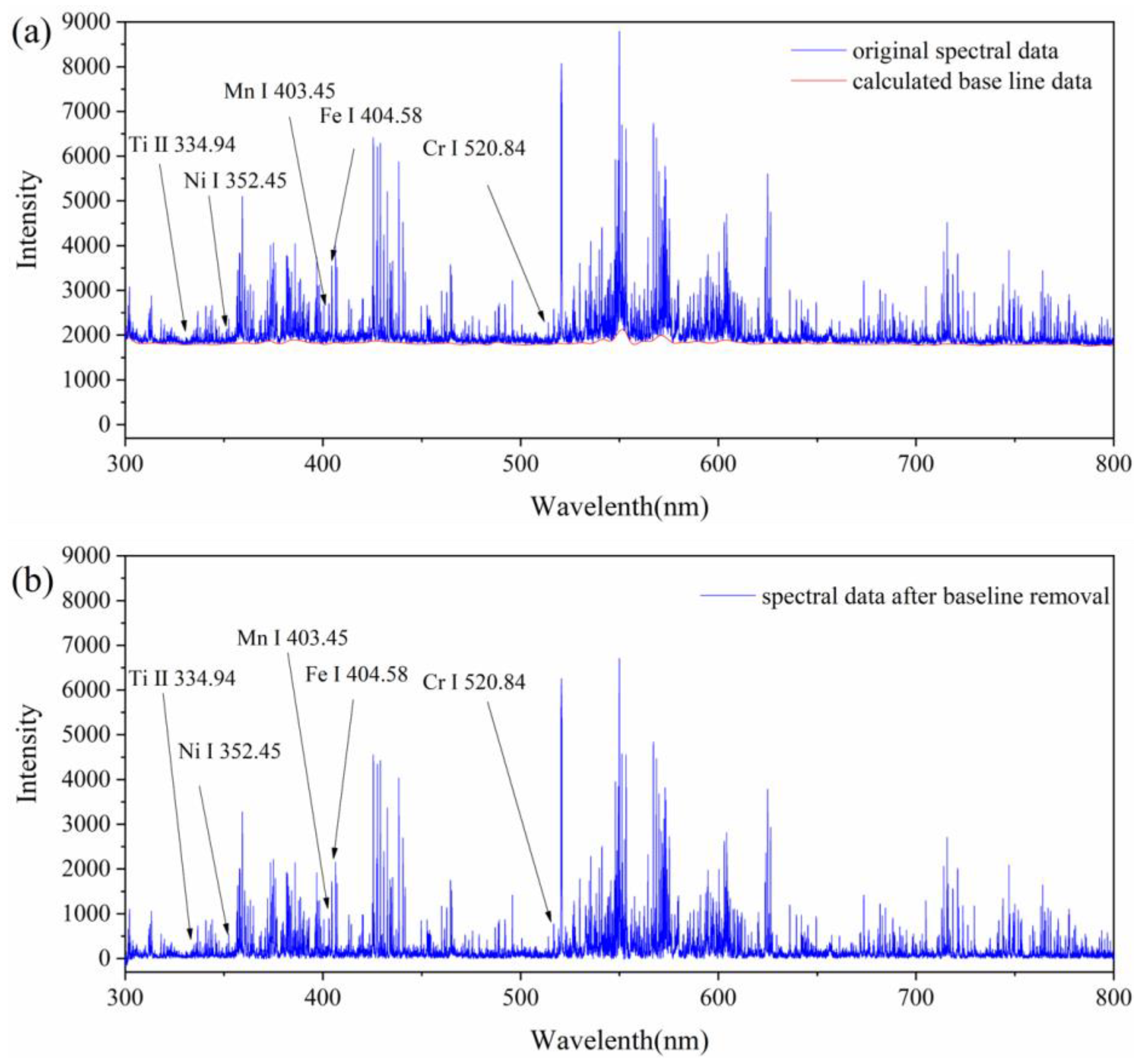
3.1. Result of Data Pre-Processing

By considering one spectrum of the sample GBW 01659a as an example, Figure 3a shows the original spectral data and calculated baseline data. Figure 3b shows the spectrum after baseline removal. In this study, the original spectral data of 33,996 data points were divided into intervals for every 300 points, and the lowest point was set as the interpolated data in each interval. Then, the baseline data were calculated by cubic spline interpolation and subtracted from the original data to obtain the spectrum without baseline. After baseline removal, the baseline of the spectrum becomes normal, and the continuous background radiation is close to zero. This implies that we can directly obtain characteristic spectral line information without continuous background noise from the spectrum.

Similarly, Figure 4a shows the spectrum after baseline removal and noise data calculated using the wavelet transform. We subtracted the data calculated by the wavelet threshold transform algorithm from the original data and obtained the denoised spectrum shown in Figure 4b in the end. During the calculation, we selected the Daubechies wavelet as the wavelet base and set the threshold to 0.03.

To evaluate the effect of denoising, we obtained Figure 5: Figure 5a shows an enlarged view of the original spectrum and baseline from 400 nm to 405 nm, while Figure 5b shows the spectrum after baseline removal and Figure 5c shows the spectrum after denoising.

The comparison showed that after baseline removal, the characteristic spectral peaks are not significantly affected. After denoising, the spectrum was smoother and the characteristic spectral lines were well preserved and became clearer. In addition, we estimated the SNR (signal-to-noise ratios) of the spectrum by dividing the peak signal value at a specific wavelength of the spectral line by the spectral noise, and the noise is defined as the root mean square on the baseline (about 20 pixels) near the peak.

Take the spectral line at 520.60 nm of Cr I as an example; the SNR of the denoised and non-denoised spectra are 23.08 and 19.03 respectively, which means wavelet transform can effectively reduce the spectral noise. This is conducive to extracting feature spectral lines in the next step to obtain more accurate results.

3.2. Feature Selection

Nine sets of spectral data were recorded for each sample. Using the database of the National Institute of Standards and Technology (NIST), we selected characteristic spectral lines with higher intensities of Ni, Cr, Ti, Si, C, and Mn. To increase the reliability of the selection of characteristic spectral lines, we calculated the Pearson correlation coefficient between the strength of the characteristic spectral lines and element content, and its expression is as follows [47]:

$$r=Cov\left(X,Y\right)/\sqrt{Var\left|X\right|Var\left|Y\right|}$$

(8)

where $X$ represents the vector of concentrations of a given element, while $Y$ represents the vector of intensities of a given line for the seven samples.

Then, spectral lines with high correlation are selected to reduce the impact of error and to obtain better prediction results.

Table 3. Selection of characteristic spectral lines of Ni, Cr, and Ti by Pearson correlation coefficient.

Species	Characteristic Spectral Lines
Ni	352.4536, 349.2956, 338.0569, 351.0335, 339.1043.
Cr	520.8426, 520.6037, 425.4336, 520.4511, 428.9717.
Ti	334.9402, 334.9033, 349.1049, 338.0277, 323.6572.

shows the top five of the selected characteristic spectral lines of such high correlations. Then, we normalized the obtained characteristic spectral line data to reduce the spectral fluctuation under repeated experiments and the influence of strange data. The normalization formula is as follows:

$$D_n=I_c/I_{Fe}$$

(9)

where $D_n$ is the normalized data, $I_c$ is the original spectral characteristic line intensity, $I_{Fe}$ is the intensity of characteristic spectral lines of major element Fe, and the Fe I line at 404.58 nm was selected here.

For comparison, we also screened the characteristic spectral lines by simply comparing them with the NIST database. The selected spectral lines are listed in

Table 4. Selection of characteristic spectral lines without Pearson correlation coefficient.

Species	Characteristic Spectral Lines
Ni	385.8297, 361.9391, 356.6372, 352.4536, 361.0462, 351.5052, 341.4764, 345.846, 346.1652, 343.3556.
Cr	520.8426, 520.6037, 520.4511, 425.4336, 427.4797, 428.9717, 357.8686, 359.3485.
Ti	375.7685, 375.9292, 390.0539, 345.6384, 346.1496, 344.4306, 349.1049, 338.027, 430.0042, 453.396.

.

3.3. Element Content Calibration by BP-ANN

We extracted the normalized peak intensity of the corresponding characteristic spectral lines of Ni, Cr, and Ti as the input variable of BP-ANN. We divided the data obtained after baseline correction, noise reduction, and feature selection and the unprocessed data into two groups. The two groups of data were used to train the model. To reduce the problems of excessively one-sided test results and insufficient training data, we divided the data of seven samples into one test set and six training sets for cross-validation. The results of seven times determination are presented in

Table 5. Determination result of Ni, Cr, and Ti with BP-ANN (Group 1).

Test Set Sample	Average Relative Error (%)			Relative Standard Deviation (%)			Root Mean Square Error (RSME)
	Ni	Cr	Ti	Ni	Cr	Ti	Ni	Cr	Ti
GBW 1659a	4.62	13.50	31.45	22.08	12.14	12.01	1.95	4.67	0.056
GBW 1660a	0.88	3.82	2.07	12.68	12.58	15.21	1.77	1.86	0.068
GBW 1661a	7.25	4.17	12.94	19.08	20.12	19.21	3.50	2.16	0.12
GBW 1662a	5.64	6.87	12.52	20.28	9.40	15.43	2.13	2.12	0.045
GBW 1663a	8.57	4.64	22.43	12.67	18.30	14.80	3.17	1.43	0.19
GBW 1664a	3.61	6.01	23.37	22.25	10.65	13.10	1.52	2.74	0.048
GBW 1665a	1.97	1.53	1.88	14.03	16.27	12.19	1.15	2.68	0.040

and

Table 6. Determination result without pre-processing (Group 2).

Test Set Sample	Average Relative Error (%)			Relative Standard Deviation (%)			Root Mean Square Error (RSME)
	Ni	Cr	Ti	Ni	Cr	Ti	Ni	Cr	Ti
GBW 1659a	8.37	15.08	26.70	25.76	9.67	28.11	1.48	2.72	0.038
GBW 1660a	5.78	8.49	10.03	17.46	18.88	22.16	2.69	3.05	0.10
GBW 1661a	15.91	4.42	42.36	21.01	17.36	24.48	4.42	1.74	0.26
GBW 1662a	9.39	11.68	22.43	20.24	8.03	19.58	2.58	2.85	0.081
GBW 1663a	13.61	11.89	28.93	23.40	22.80	13.94	3.11	2.13	0.24
GBW 1664a	10.70	8.27	61.54	26.57	9.70	18.38	2.19	2.88	0.12
GBW 1665a	8.79	2.18	16.73	29.31	15.78	17.52	1.73	2.60	0.086

. The predicted value is the result of predicting the elemental content from different spectral data. Then, the average relative error (ARE), relative standard deviation (RSD), and root mean square error (RSME) were calculated as evaluation parameters.

In addition, Figure 6 shows the learning curve of BP-ANN in Ni calibration, from which we can see the mean square error (MSE) of the training and testing sets with different training data. For the curve drawing, one test sample was used. Figure 7 shows the loss curves, indicating the variation of training loss, and validation loss with epochs. It can be seen that the training and testing results are good, and the loss curve converges effectively, indicating that the model fits well and has some generalization ability.

In general, the prediction results of Group 1 (Table 4) are more accurate by comparison. In particular, for the determination of Ni, the average error in Group 1 was within 9%. For most samples, the error in the determination of elemental Cr is within 7%. This means that when the LIBS data are pre-processed by the above method, fewer spectral lines were used for training, which can significantly improve the training efficiency.

However, the errors in the determination of the concentrations of elemental Cr for sample GBW 1659a and of elemental Ti for most samples were substantial. Possible reasons for this are as follows: on the one hand, we found that the model did not fit well for individual training sets in the cross-validation due to insufficient sample and data volume. On the other hand, the element Ti was insufficiently present in the stainless steel samples (<1 wt%), making its characteristic spectral lines indistinguishable and fluctuated, and thus difficult to determine. In addition, low peaks containing information mixed with the noise may be removed during data pre-processing. However, the lines selected by the algorithm still obtain a high correlation with the element concentrations, which is an interesting topic worth further study.

The RSD reflects the precision and repeatability of the results. We can see that the stability and precision of the predicted Ni and Ti concentrations are higher in Group 1 data than in Group 2 data. The overall RSD of the BP-ANN results are still high, probably due to the complex and unstable LIBS data. However, in this study, the data pre-processing method demonstrates certain advantages over RSD.

3.4. Comparison of Quantitative Methods

The same data (Group 1) were used to predict the elemental concentrations of Ni, Cr, and Ti by support vector regression (SVR), partial least squares regression (PLSR), and univariate least squares regression (ULSR). These models have also been optimized, and the average of the resulting ARE is given in Figure 8.

In this study, SVR and PLSR are both built on Scikit-learn. The kernel type of SVR is set as “Linear,” the penalty factor C is set to 3.0, and the parameter “n_components” of PLSR is set to 4. ULSR performs a linear fit with the intensity and elemental content of the characteristic spectral lines of the training sets as variables.

Obviously, the BP-ANN results are more accurate than SVR, PLSR, and ULSR and include better results for Group 1 data than for Group 2 data, and the averages of ARE of predicted concentrations by BP-ANN are less than 6%. This shows that the pre-processing method we used effectively improves the performance of BP-ANN. In addition, BP-ANN has an advantage over SVR, PLSR, and ULSR and is more suitable for the pre-processing method in this study. Furthermore, the SVM model performs well and has some promise as a quantitative model for LIBS.

4. Discussion and Conclusions

As shown in Table 1, the superiority of BP-ANN combined with LIBS for rapid elemental analysis has been demonstrated and various samples have been studied. Compared with contemporary studies, this study focuses on the improvement in LIBS data pre-processing to enhance the prediction performance of BP-ANN. Cubic spline interpolation and wavelet threshold transform algorithms were used to perform baseline removal and denoising of LIBS spectral data, respectively, and the characteristic spectral lines were selected using the Pearson correlation coefficient. This method can automatically process the original spectrum data into characteristic emission spectrum information and remove interference information, which can increase the analyzing speed of BP-ANN with complicated spectra of alloy. Moreover, this method is fast and uncomplicated.

In conclusion, BP-ANN combined with a data pre-processing method to analyze the LIBS spectra was proposed. In addition, seven standard stainless steel samples for spectral analyzing (GBW 01659a, GBW 01660a, GBW 01661a, GBW 01662a, GBW 01663a, GBW 01664a, and GBW 01665a) were used. After pre-processing, the baseline was corrected and the noise of the spectrum was reduced, resulting in a higher signal-to-noise ratio, thus illustrating the effectiveness of the noise reduction method. By comparing the BP-ANN training results for the pre-processed and unprocessed data, the former prediction results are more accurate. The average error in the determination of Ni is within 9%, while in the determination of Cr, it is mostly within 7%. The RSDs of the results for Ni and Ti elements were generally lower in the former, indicating that the pre-processing method can improve the stability of the predictions for Ni and Ti. We then compared the mean error of the quantitative prediction results of the four methods BP-ANN, SVR, PLSR, and ULSR, showing that BP-ANN is more accurate in predicting the concentrations of Ni, Cr and Ti in stainless steel when combined with this pre-processing method. This means that the determination method is promising for the practical detection of minor elements in stainless steel samples.

References

1. Rusak, D.; Castle, B.; Smith, B.; Winefordner, J. Fundamentals and applications of laser-induced breakdown spectroscopy. Crit. Rev. Anal. Chem. 1997, 27, 257–290. [Google Scholar] [CrossRef]
2. Brech, F.; Cross, L. Optical microemission stimulated by a ruby maser. Appl. Spectmsc. 1962, 16, 59–64. [Google Scholar]
3. Hu, Y.; Li, Z.; Lü, T. Determination of elemental concentration in geological samples using nanosecond laser-induced breakdown spectroscopy. J. Anal. At. Spectrom. 2017, 32, 2263–2270. [Google Scholar] [CrossRef]
4. Tucker, J.; Dyar, M.; Schaefer, M.; Clegg, S.; Wiens, R. Optimization of laser-induced breakdown spectroscopy for rapid geochemical analysis. Chem. Geol. 2010, 277, 137–148. [Google Scholar] [CrossRef]
5. Chen, T.; Zhang, T.; Li, H. Applications of laser-induced breakdown spectroscopy (LIBS) combined with machine learning in geochemical and environmental resources exploration. Trends Anal. Chem. 2020, 133, 116113. [Google Scholar] [CrossRef]
6. De Lucia, F.C., Jr.; Gottfried, J.L. Influence of variable selection on partial least squares discriminant analysis models for explosive residue classification. Spectrochim. Acta Part B 2011, 66, 122–128. [Google Scholar] [CrossRef]
7. Horňáčková, M.; Grolmusová, Z.; Horňáček, M.; Rakovský, J.; Hudec, P.; Veis, P. Calibration analysis of zeolites by laser induced breakdown spectroscopy. Spectrochim. Acta Part B 2012, 74, 119–123. [Google Scholar] [CrossRef]
8. Kondo, H.; Aimoto, M.; Yamamura, H.; Toh, T. Rapid defect characterization of steel by laser induced breakdown spectroscopy. Metall. Anal. 2009, 29, 13–16. [Google Scholar]
9. Hamzaoui, S.; Khleifia, R.; Jaïdane, N.; Lakhdar, Z.B. Quantitative analysis of pathological nails using laser-induced breakdown spectroscopy (LIBS) technique. Lasers Med. Sci. 2011, 26, 79–83. [Google Scholar] [CrossRef]
10. Nicolodelli, G.; Cabral, J.; Menegatti, C.R.; Marangoni, B.; Senesi, G.S. Recent advances and future trends in LIBS applications to agricultural materials and their food derivatives: An overview of developments in the last decade (2010–2019). Part I. Soils and fertilizers. Trends Anal. Chem. 2019, 115, 70–82. [Google Scholar] [CrossRef]
11. Qi, J.; Zhang, T.; Tang, H.; Li, H. Rapid classification of archaeological ceramics via laser-induced breakdown spectroscopy coupled with random forest. Spectrochim. Acta Part B 2018, 149, 288–293. [Google Scholar] [CrossRef]
12. Zhang, Y.; Zhang, T.; Li, H. Application of laser-induced breakdown spectroscopy (LIBS) in environmental monitoring. Spectrochim. Acta Part B 2021, 181, 106218. [Google Scholar] [CrossRef]
13. Hsu, P.S.; Gragston, M.; Wu, Y.; Zhang, Z.; Patnaik, A.K.; Kiefer, J.; Roy, S.; Gord, J.R. Sensitivity, stability, and precision of quantitative Ns-LIBS-based fuel-air-ratio measurements for methane-air flames at 1–11 bar. Appl. Opt. 2016, 55, 8042–8048. [Google Scholar] [CrossRef] [PubMed]
14. Stipe, C.B.; Hensley, B.D.; Boersema, J.L.; Buckley, S.G. Laser-induced breakdown spectroscopy of steel: A comparison of univariate and multivariate calibration methods. Appl. Spectmsc. 2010, 64, 154–160. [Google Scholar] [CrossRef]
15. Xu, X.; Du, C.; Ma, F.; Shen, Y.; Zhou, J. Fast and simultaneous determination of soil properties using laser-induced breakdown spectroscopy (LIBS): A case study of typical farmland soils in China. Soil Syst. 2019, 3, 66. [Google Scholar] [CrossRef] [Green Version]
16. Zhang, Y.; Sun, C.; Gao, L.; Yue, Z.; Shabbir, S.; Xu, W.; Wu, M.; Yu, J. Determination of minor metal elements in steel using laser-induced breakdown spectroscopy combined with machine learning algorithms. Spectrochim. Acta Part B 2020, 166, 105802. [Google Scholar] [CrossRef]
17. Li, L.-N.; Liu, X.-F.; Yang, F.; Xu, W.-M.; Wang, J.-Y.; Shu, R. A review of artificial neural network based chemometrics applied in laser-induced breakdown spectroscopy analysis. Spectrochim. Acta Part B 2021, 180, 106183. [Google Scholar] [CrossRef]
18. Li, K.; Guo, L.; Li, C.; Li, X.; Shen, M.; Zheng, Z.; Yu, Y.; Hao, R.; Hao, Z.; Zeng, Q. Analytical-performance improvement of laser-induced breakdown spectroscopy for steel using multi-spectral-line calibration with an artificial neural network. J. Anal. At. Spectrom. 2015, 30, 1623–1628. [Google Scholar] [CrossRef]
19. Rezaei, F.; Karimi, P.; Tavassoli, S. Effect of self-absorption correction on LIBS measurements by calibration curve and artificial neural network. Appl. Phys. B 2014, 114, 591–600. [Google Scholar] [CrossRef]
20. Sirven, J.-B.; Bousquet, B.; Canioni, L.; Sarger, L. Laser-induced breakdown spectroscopy of composite samples: Comparison of advanced chemometrics methods. Anal. Chem. 2006, 78, 1462–1469. [Google Scholar] [CrossRef]
21. M Motto-Ros, V.; Koujelev, A.S.; Osinski, G.R.; Dudelzak, A.E. Quantitative Multi-Elemental Laser-Induced Breakdown Spectroscopy Using Artificial Neural Networks. J. Eur. Opt. Soc. Rapid Publ. 2008, 3, 8011. [Google Scholar] [CrossRef]
22. Inakollu, P.; Philip, T.; Rai, A.K.; Yueh, F.-Y.; Singh, J.P. A comparative study of laser induced breakdown spectroscopy analysis for element concentrations in aluminum alloy using artificial neural networks and calibration methods. Spectrochim. Acta Part B 2009, 64, 99–104. [Google Scholar] [CrossRef]
23. D’Andrea, E.; Pagnotta, S.; Grifoni, E.; Lorenzetti, G.; Legnaioli, S.; Palleschi, V.; Lazzerini, B. An artificial neural network approach to laser-induced breakdown spectroscopy quantitative analysis. Spectrochim. Acta Part B 2014, 99, 52–58. [Google Scholar] [CrossRef]
24. Moncayo, S.; Manzoor, S.; Rosales, J.; Anzano, J.; Caceres, J. Qualitative and quantitative analysis of milk for the detection of adulteration by Laser Induced Breakdown Spectroscopy (LIBS). Food Chem. 2017, 232, 322–328. [Google Scholar] [CrossRef] [PubMed] [Green Version]
25. Yang, P.; Li, X.; Nie, Z. Determination of the nutrient profile in plant materials using laser-induced breakdown spectroscopy with partial least squares-artificial neural network hybrid models. Opt. Express 2020, 28, 23037–23047. [Google Scholar] [CrossRef] [PubMed]
26. Safi, A.; Campanella, B.; Grifoni, E.; Legnaioli, S.; Lorenzetti, G.; Pagnotta, S.; Poggialini, F.; Ripoll-Seguer, L.; Hidalgo, M.; Palleschi, V. Multivariate calibration in Laser-Induced Breakdown Spectroscopy quantitative analysis: The dangers of a ‘black box’approach and how to avoid them. Spectrochim. Acta Part B 2018, 144, 46–54. [Google Scholar] [CrossRef] [Green Version]
27. ZHANG, T.-L.; Shan, W.; Hong-Sheng, T.; Kang, W.; Yi-Xiang, D.; Hua, L. Progress of chemometrics in laser-induced breakdown spectroscopy analysis. Chin. J. Anal. Chem. 2015, 43, 939–948. [Google Scholar] [CrossRef]
28. Tan, Z.; Tao, Z.; Liu, J.; Wang, G. Baseline correction of roman spectrum based on piecewise linear fitting. Spectrosc. Spectr. Anal. 2013, 33, 383–386. [Google Scholar] [CrossRef]
29. Weakley, A.T.; Griffiths, P.R.; Aston, D.E. Automatic baseline subtraction of vibrational spectra using minima identification and discrimination via adaptive, least-squares thresholding. Appl. Spectmsc. 2012, 66, 519–529. [Google Scholar] [CrossRef]
30. Sun, L.; Yu, H. Automatic estimation of varying continuum background emission in laser-induced breakdown spectroscopy. Spectrochim. Acta Part B 2009, 64, 278–287. [Google Scholar] [CrossRef] [Green Version]
31. Tan, B.; Huang, M.; Zhu, Q.; Guo, Y.; Qin, J. Detection and correction of laser induced breakdown spectroscopy spectral background based on spline interpolation method. Spectrochim. Acta Part B 2017, 138, 64–71. [Google Scholar] [CrossRef]
32. Zhang, B.; Sun, L.; Yu, H.; Xin, Y.; Cong, Z. A method for improving wavelet threshold denoising in laser-induced breakdown spectroscopy. Spectrochim. Acta Part B 2015, 107, 32–44. [Google Scholar] [CrossRef]
33. Yuan, T.; Wang, Z.; Li, Z.; Ni, W.; Liu, J. A partial least squares and wavelet-transform hybrid model to analyze carbon content in coal using laser-induced breakdown spectroscopy. Anal. Chim. Acta 2014, 807, 29–35. [Google Scholar] [CrossRef]
34. Swindeman, R.; Sikka, V.; Klueh, R. Residual and trace element effects on the high-temperature creep strength of austenitic stainless steels. Metall. Trans. A 1983, 14, 581–593. [Google Scholar] [CrossRef]
35. Melford, D. The influence of residual and trace elements on hot shortness and high temperature embrittlement. Philos. Trans. R. Soc. Lond. Ser. A 1980, 295, 89–103. [Google Scholar] [CrossRef]
36. Senesi, G.S.; De Pascale, O.; Bove, A.; Marangoni, B.S. Quantitative Analysis of Pig Iron from Steel Industry by Handheld Laser-Induced Breakdown Spectroscopy and Partial Least Square (PLS) Algorithm. Appl. Sci. 2020, 10, 8461. [Google Scholar] [CrossRef]
37. Li, J.; Liu, X.; Li, X.; Ma, Q.; Zhao, N.; Zhang, Q.; Guo, L.; Lu, Y. Investigation of excitation interference in laser-induced breakdown spectroscopy assisted with laser-induced fluorescence for chromium determination in low-alloy steels. Opt. Lasers Eng. 2020, 124, 105834. [Google Scholar] [CrossRef]
38. Zhang, W.; Zhou, R.; Liu, K.; Li, Q.; Tang, Z.; Zhu, C.; Li, X.; Zeng, X.; He, C. Silicon determination in steel with molecular emission using laser-induced breakdown spectroscopy combined with laser-induced molecular fluorescence. J. Anal. At. Spectrom. 2021, 36, 375–379. [Google Scholar] [CrossRef]
39. Cui, M.; Guo, H.; Chi, Y.; Tan, L.; Yao, C.; Zhang, D.; Deguchi, Y. Quantitative analysis of trace carbon in steel samples using collinear long-short double-pulse laser-induced breakdown spectroscopy. Spectrochim. Acta Part B 2022, 191, 106398. [Google Scholar] [CrossRef]
40. Wang, Z.; Feng, J.; Li, L.; Ni, W.; Li, Z. A multivariate model based on dominant factor for laser-induced breakdown spectroscopy measurements. J. Anal. At. Spectrom. 2011, 26, 2289–2299. [Google Scholar] [CrossRef]
41. Chun-Long, W.; Jian-Guo, L.; Nan-Jing, Z.; Ming-Jun, M.; Yin, W.; Li, H.; Da-Hai, Z.; Yang, Y.; De-Shuo, M.; Wei, Z. Comparative analysis of quantitative method on heavy metal detection in water with laser-induced breakdown spectroscopy. Acta Phys. Sin. 2013, 62, 125201. [Google Scholar] [CrossRef]
42. Guo, Y.-M.; Guo, L.-B.; Li, J.-M.; Liu, H.-D.; Zhu, Z.-H.; Li, X.-Y.; Lu, Y.-F.; Zeng, X.-Y. Research progress in Asia on methods of processing laser-induced breakdown spectroscopy data. Front. Phys. 2016, 11, 114212. [Google Scholar] [CrossRef]
43. Kouibia, A.; Pasadas, M. An approximation problem of noisy data by cubic and bicubic splines. Appl. Math. Model. 2012, 36, 4135–4145. [Google Scholar] [CrossRef]
44. Lu, P.; Zhuo, Z.; Zhang, W.; Tang, J.; Tang, H.; Lu, J. Accuracy improvement of quantitative LIBS analysis of coal properties using a hybrid model based on a wavelet threshold de-noising and feature selection method. Appl. Opt. 2020, 59, 6443–6451. [Google Scholar] [CrossRef]
45. Ciucci, A.; Corsi, M.; Palleschi, V.; Rastelli, S.; Salvetti, A.; Tognoni, E. New procedure for quantitative elemental analysis by laser-induced plasma spectroscopy. Appl. Spectmsc. 1999, 53, 960–964. [Google Scholar] [CrossRef]
46. Yan, C.; Zhang, T.; Sun, Y.; Tang, H.; Li, H. A hybrid variable selection method based on wavelet transform and mean impact value for calorific value determination of coal using laser-induced breakdown spectroscopy and kernel extreme learning machine. Spectrochim. Acta Part B 2019, 154, 75–81. [Google Scholar] [CrossRef]
47. Adler, J.; Parmryd, I. Quantifying colocalization by correlation: The Pearson correlation coefficient is superior to the Mander’s overlap coefficient. Cytom. Part A 2010, 77, 733–742. [Google Scholar] [CrossRef]
Figure 1. Schematic of the experimental setup.
Chemosensors 10 00472 g001
Figure 2. Structure of BP-ANN with three layers.
Chemosensors 10 00472 g002
Figure 3. LIBS spectrum of sample GBW 01659a in the wavelength range of 300–800 nm: (a) the original spectral data (blue line) and calculated baseline data based on cubic spline interpolation algorithm (red line); (b) the spectral data after baseline removal obtained by subtracting the baseline data from the original data.
Chemosensors 10 00472 g003
Figure 4. LIBS spectrum of sample GBW 01659a in the wavelength range of 300–800 nm: (a) the spectral data after baseline removal (blue line, same as Figure 3b) and noise data calculated by wavelet transform (red line); (b) the data after denoising, obtained via subtracting the noise data from the data after baseline removal.
Chemosensors 10 00472 g004
Figure 5. Enlarged view of the LIBS spectrum of sample GBW 01659a in the wavelength range of 400–405 nm: (a) the original spectral data (blue line) and calculated baseline data by cubic spline interpolation algorithm (red line); (b) the spectral data after baseline removal; (c) the data after denoising, obtained by subtracting the noise data from the data after baseline removal.
Chemosensors 10 00472 g005
Figure 6. Learning curve of BP-ANN: variation in MSE with number of training samples for training sets (red line) and test sets (black line).
Chemosensors 10 00472 g006
Figure 7. Loss curves of BP-ANN: variation in training loss and validation loss with epochs.
Chemosensors 10 00472 g007
Figure 8. Comparison of different quantitative methods: the average of ARE of predicted results by BP-ANN, SVR, PLSR, and ULSR.
Chemosensors 10 00472 g008