Article

A Comparative Study of the Method to Rapid Identification of the Mural Pigments by Combining LIBS-Based Dataset and Machine Learning Methods

1
Key Laboratory of Atomic and Molecular Physics & Functional Materials of Gansu Province, College of Physics and Electronic Engineering, Northwest Normal University, Lanzhou 730070, China
2
National Research Centre for Conservation of Ancient Wall Paintings and Earthen Sites, Dunhuang 736200, China
*
Authors to whom correspondence should be addressed.
Chemosensors 2022, 10(10), 389; https://doi.org/10.3390/chemosensors10100389
Submission received: 1 August 2022 / Revised: 9 September 2022 / Accepted: 21 September 2022 / Published: 24 September 2022
(This article belongs to the Special Issue Application of Laser-Induced Breakdown Spectroscopy)

Abstract

:
Due to the similar chemical composition and matrix effect, the accurate identification of mineral pigments on wall paintings has brought great challenges. This work implemented an identification study on three mineral pigments with similar chemical compositions by combining LIBS technology with the K-nearest neighbor algorithm (KNN), random forest (RF support vector machine (SVM), back propagation artificial neural network (Bp-ANN) and convolutional neural network (CNN) to find the most suitable identification method for mural research. Using the SelectKBest algorithm, 300 characteristic lines with the largest difference among the three pigments were determined. The identification models of KNN, RF, SVM, Bp-ANN and CNN were established and optimized. The results showed that, except for the KNN model, the identification accuracy of other models for mock-up mural samples was above 99%. However, only the identification accuracy of 2D-CNN models reached above 94% for actual mural samples. Therefore, the 2D-CNN model was determined as the most suitable model for the identification and analysis of mural pigments.

1. Introduction

Dunhuang Mogao Grottoes preserve the world’s largest and most complete exquisite murals [1]. Due to various natural disasters and human factors, the murals have very serious degradation, which makes it difficult for relevant personnel to analyze, protect and extract historical information. For example, different shades of green in the same mural are actually the same pigment. Moreover, due to the similar elemental composition and complex matrix effects of some pigments [2], it is challenging to identify different mineral pigments by spectroscopy. At the same time, the production process of the Dunhuang murals has not been recorded, and the in situ analysis data of mineral pigments are missing. Therefore, an efficient and accurate identification method is urgently needed to provide important reference and data support for mural protection, restoration and material identification.
In recent years, many detection techniques have been applied to mural detection, such as Fourier transform infrared spectroscopy (FT-IR) [3], Raman spectroscopy (Raman) [4], X-ray diffraction (XRD) [5] and more. For murals unable to be moved, such as the multi-layer structure murals of Mogao Grottoes, they have some limits, such as the detection range [6], serious surface organic interference [7] and the need for vacuum conditions [8]. Although some portable spectrometers have been used for in situ analysis in caves, the depth of measurement cannot be controlled [9]. Laser-induced breakdown spectroscopy (LIBS) has the advantages of a no-sample preparation and pretreatment, simultaneous multi-element simultaneous measurement, in situ analysis and multi-layer structure information analysis, which fully meets the detection requirements of Mogao Grottoes murals. Before this work, we conducted some meaningful studies on Mogao Grottoes murals [10,11,12]. For example, by coupling with the principal component analysis (PCA) method, a classifiable pigment size model was constructed and successfully applied to the pigment size classification on real murals. LIBS was used for depth profile analysis of green coatings by combining cross-sectional analysis with optical microscopy to obtain a fitting relationship between ablation depth and laser ablation pulse number.
Due to the influence of laser energy unsteadiness, sample surface evenness and matrix effect on LIBS characteristic spectrum [13,14,15], LIBS technology is often combined with the advanced machine learning model based on multivariate statistical technology to improve the identification accuracy of materials with similar chemical compositions. Qi et al. [16] successfully classified ceramics of different ages by combining LIBS technology with random forests. Duchene et al. [17] significantly improved the recognition rate of unknown spectra obtained in the laboratory by combining soft independent modeling of class analogy (SIMCA) and partial least-squares discriminant analysis (PLS-DA). In order to promote the separation of different binders used in murals, Bai et al. [18] used LIBS and PCA to prove that 266 nm laser wavelength can obtain better performance.
As a special machine learning method, deep learning has unique advantages in feature selection, neural network training and high-dimensional data processing [19,20], among which convolutional neural network (CNN) is one of the most widely used deep learning models. Sang et al. [21], through the combination of Raman technology and CNN, realized the identification of the mineral Raman spectrum in the RRUFF dataset and obtained high accuracy.
In this study, LIBS spectral data were combined with five machine learning methods for the first time, including K-nearest neighbor (KNN), RF, SVM, Bp-ANN and CNN, which were applied to mineral pigments with similar chemical compositions. It provided a new method for rapid in situ recognition of mural pigments. Using the SelectKBest algorithm, 300 characteristic lines with the largest difference among the three pigments were determined. The identification models of KNN, RF, SVM, Bp-ANN and two-dimensional convolutional neural network (2D-CNN) were established and optimized. The 2D-CNN model was determined as the most suitable model for the identification and analysis of mural pigments.

2. Experiment and Methods

2.1. Experimental Setup
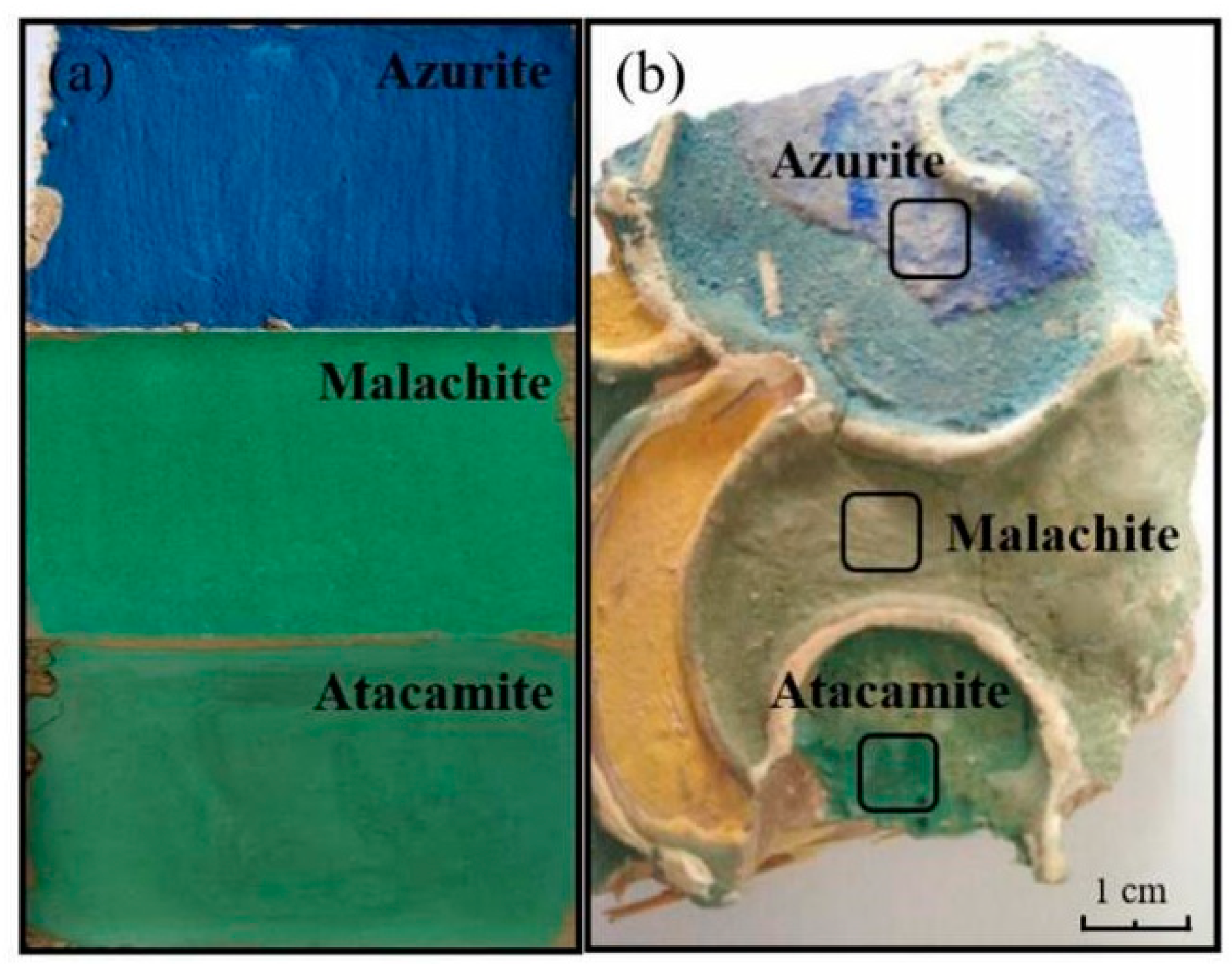
A detailed description of the experimental device and its central part was the same as our previous work [22]. Briefly, a laser (Dawa-100, Beamtech Co., Ltd., Beijing, China) at 1064 nm delivered 5 ns and 10 mJ laser pulses to the samples after being focused by a lens of 100 mm focal length for the LIBS measurements. The sample was fixed on an XYZ-3D linear stage so that the laser could ablate different positions. A center-to-center distance of 0.5 mm was left between neighboring craters. After plasma was induced on the sample, a convergent lens was placed at a 45° angle with respect to the laser beam direction to focus the plasma emission signal. Then the signal was collected by an echelle grating spectrometer (LTB, ARYELLE200) using optical fiber and detected using the intensified charge-coupled device (ICCD) detector.

2.2. Samples

Due to the preciousness of murals, spectral data could not be collected in large quantities on the actual murals. Therefore, we needed to make mock-up mural samples in the laboratory, as shown in Figure 1a. The pigments used were made according to the traditional mineral pigment processing method in Lhasa, Tibet. To ensure that the pigments were consistent with those used in the actual murals, the compositions of these mineral pigments were tested using the XRD and FT-IR techniques. This method can be found in our previous work [22]
In this experiment, three kinds of mineral pigments were selected. Mineral pigments are not adhesive, so the ancients usually added binding media. Therefore, to reproduce the secco technology used in the Mogao Grottoes, the production process of mock-up mural samples was divided into material preparation, plaster layer production, binding media solution preparation and painted layer production. The area of the paint layer was 4 × 2 cm2, and the thickness was 2 mm. These relatively thick painting layers ensure that the collected LIBS spectral data only contained information from the painting layer.
We collected a fragment of a collapsed Buddha statue in a cave for experimental analysis, which can be traced back to the Yuan Dynasty, to successfully apply the identification methods to in situ analysis. We studied three areas of the painted layer on the mural fragment, which were azurite, malachite and atacamite, as shown in Figure 1b. The fragment is currently stored in the laboratory of the Dunhuang Research Institute.

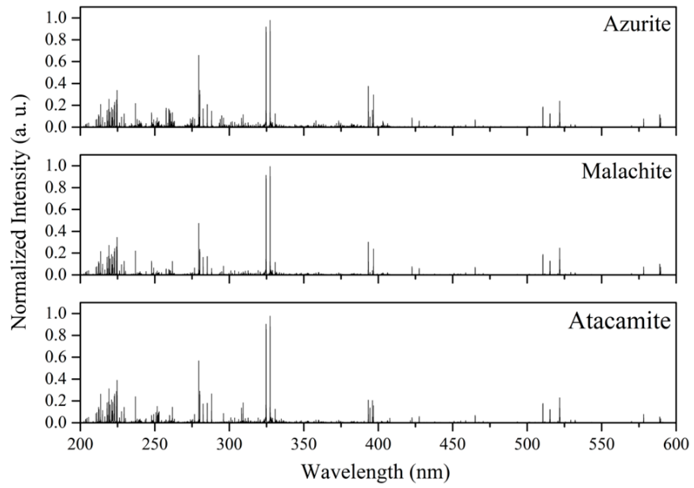
2.3. Spectral Acquisition and Data Processing

In this work, two mock-up mural samples were prepared for each pigment, and 200 and 100 spectral data were measured, respectively. A total of 900 spectra were collected, of which 600 spectra were the training set and 300 spectra were the test set of the mock-up mural samples. All spectra of the training set were the result of five accumulated scans, and the two times were averaged to reduce the unsteadiness caused by the laser pulse energy jitter. The spectral intensity range was adjusted between 0 and 1 by min-max normalization to reduce the system load and speed up the algorithm process.
Although the actual mural fragments are very precious, to ensure the accuracy of the model in situ analysis, we needed to collect 50 LIBS spectra in each of the three regions of the actual mural fragment. Figure 2 shows the classic LIBS spectra of three mineral pigments with Cu as the main element. The chemical formulas of azurite, malachite and atacamite are 2CuCO3·Cu(OH)2, Cu2CO3(OH)2 and Cu2(OH)3Cl, respectively. The difference in their chemical formulas was very small, and in the process of laser ablation, the main element of the three pigments was Cu, while LIBS technology only reflected the elemental composition, which makes their LIBS spectra similar.
The characteristic spectral lines intensity of several main elements in three mineral pigments was obvious, and the same trend was shown, which brought some challenges to the classified work.

2.4. Methods

2.4.1. K-Nearest Neighbor

KNN identification [23,24] is one of the most fundamental and simple identification methods, which is widely used in character recognition, text identification, image recognition and other fields. When KNN performs the identification task, the model measures the distance from an unknown sample set to each known sample set. Then K-known samples nearest to the unknown sample set are selected to let each neighbor “vote”, and the unknown samples are classified as the type with the largest proportion among the K-neighboring samples.
The advantages of this method are simple structure, short training time and usefulness for identification and regression problems. When the number of samples is not balanced, it is difficult due to the small number of samples.

2.4.2. Support Vector Machine

SVM [25,26] is one of the most influential methods in supervised learning, which is a machine learning method based on statistical learning theory. It can construct hyperplanes or hyperplane sets in high-dimensional space and be used for identification, regression or other tasks. For two-dimensional data, the hyperplane is the line between two categories that most effectively separates the data. The test points or query points are then mapped into that same space and predicted to belong to a category based on which side of the gap they fall on.
This is its strength that can effectively solve computational complexity and high-dimensional problems, and it also has a better effect in dealing with nonlinear questions. But it is less sensitive to data, and difficult to find a suitable kernel function for nonlinear problems.

2.4.3. Random Forest

RF [27,28] is one of the most used machine learning ensembles. RF builds a forest with many decision trees from randomly extracting training data. Each decision tree can give the identification output of unknown test samples. Lastly, according to the identification output results of all decision trees, the final identification output of the unknown test sample is provided. If a category obtains more output times, the unknown test sample is more likely to belong to it.
Its calculation process is simple and advantageous to understanding and interpretation; but it is easy for overfitting phenomena to occur. Moreover, when the number of samples is inconsistent, the results of information acquisition tend to be the type with more samples in the decision tree.

2.4.4. Back Propagation Artificial Neural Network

Bp-ANN [29,30] is one of the most classical neural network models, which trains the identification model through feedforward calculation and backpropagation calculation. It is composed of input, hidden and output layers, which are responsible for information input, information transfer, cumulative calculation, and information output, respectively.
Its advantages are high identification accuracy, outstanding storage, learning ability and excellent memory ability. However, the deficiencies are that the training time is long and the learning process cannot be observed; more arguments are needed.

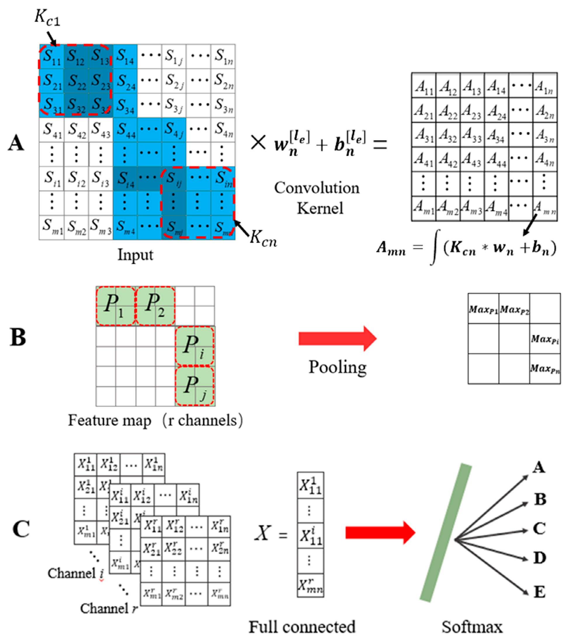
2.4.5. Convolutional Neural Network

CNN [31,32] is a feedforward neural network with convolution calculation and deep structure, which is generally composed of input, convolution, pooling and full connection layers.
The first layer of CNN is the input layer that contains the spectral data. Since 2D-CNN is used in this work, CNN employs a matrix as input (in 1D-CNN, CNN employs a vector as input). Then, each input is convolved with a convolution kernel matrix of 3 × 3, and the feature matrix with relatively few values is obtained. All these values will constitute a new output feature matrix by introducing the activation function. Figure 3a shows how the convolution kernel performed feature extraction.
The pooling layer is mainly applied to reduce the dimension of the feature matrices and the number of network parameters. This work uses maximum pooling. After extracting features in the convolution layers, the 2 × 2 matrix is used to further reduce the dimension of the feature matrices. This process only extracts the maximum value in each matrix to filter out useless information. In this way, it is possible to simplify the complexity of the neural network and improve the operation speed. Figure 3b shows how the max-pooling layers are employed to scan the feature matrices.
Then, the extracted feature information is flattened into a vector, and the identification task is completed through the full connection layer according to the weight matrix and deviation parameters. Finally, the vector is entered into the final layer, and the probability of corresponding categories of each test sample is obtained by the Softmax function. Figure 3c shows the flattening process and how a fully connected classifier is employed to classify the information extracted from the previous convolution and max-pooling layers.
CNN can lightly process high-dimensional data and automatically extract feature information. Nonetheless, valuable information may be lost in the pooling layer, and the increase in network structure may lead to longer computing time.

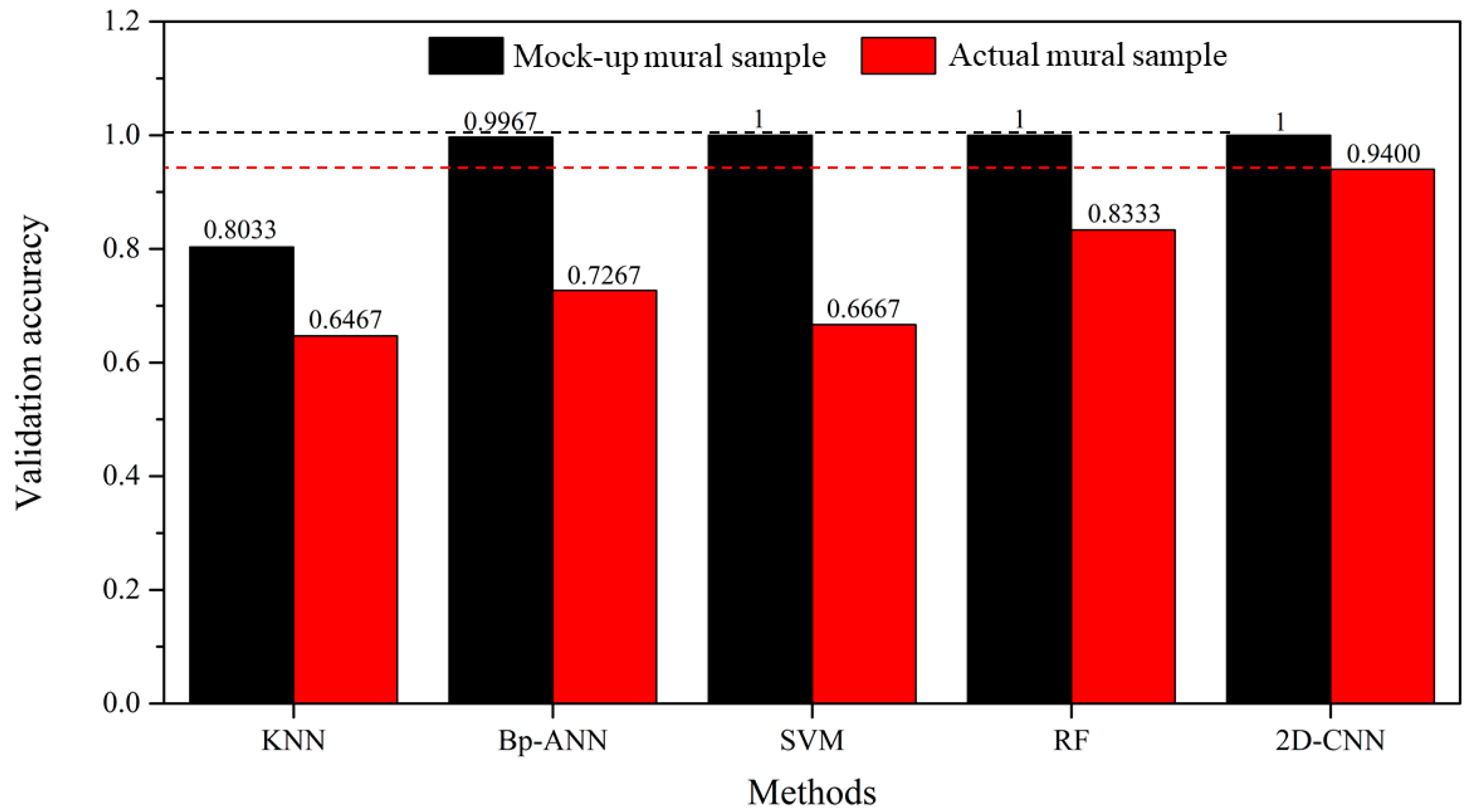
3. Results and Discussion

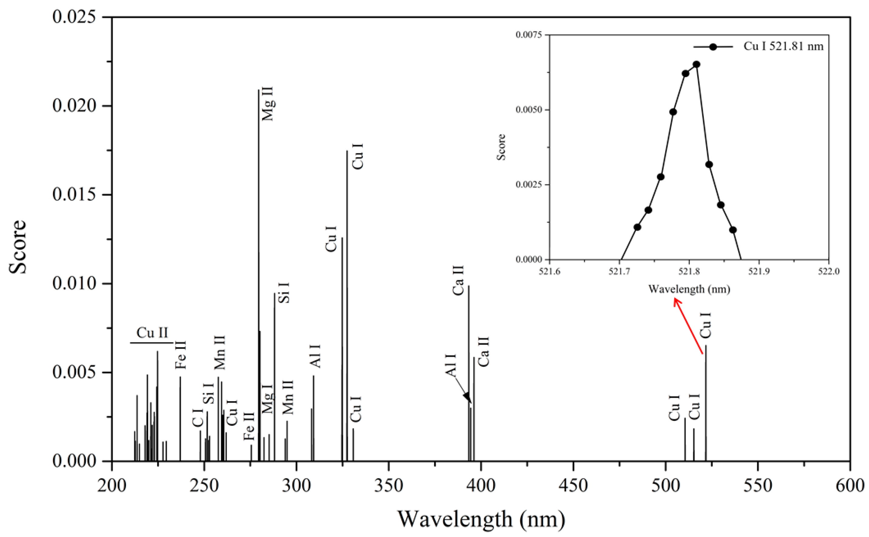
3.1. Spectral Feature Selection

Considering that the number of input features is not only directly related to the accuracy of model identification but also affects the computational efficiency, the SelectKBest algorithm was selected to select the best feature set for the subsequent data analysis process [33]. The difference between the three types of samples was determined by calculating the correlation between the intensity of each spectral pixel and the intensity of all training spectral pixels. And the advantage of this method is that it can reduce the data dimension and ensure the main difference information of the spectrum. The correlation between 42,841 pixels in the spectrum was calculated, and the spectral pixels scored in the top 300 were retained. These pixels will be used as characteristic wavelengths in the training set and test set to ensure the spectral characteristics of the whole operation process are consistent.
The results of feature selections are shown in Figure 4. The spectral differences are mainly Cu I, Cu II, Fe II, CI, Mn II, Si I, Al I and Mg II. This indicated that trace elements play a leading role in the identification process. The spectral contour of Cu I 521.81 nm is amplified and displayed To more clearly see the pixels that constitute the spectral contour.

3.2. Construction and Optimization of Machine Learning Models

All the models used in this work were verified by a five-fold cross-validation method to ensure the reliability and generalization ability of the classified results. The training set was divided into five parts, taking turns to train four parts and then verifying one part. The accuracy of the algorithm can be obtained by averaging the five results.

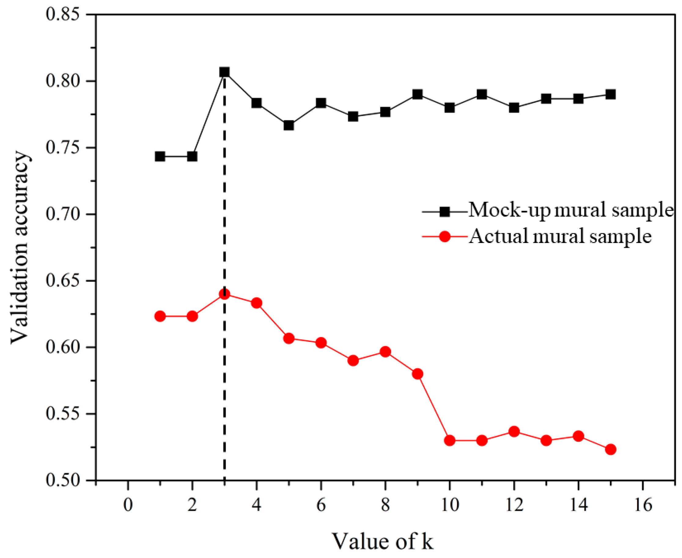
3.2.1. K-Nearest Neighbor

In this part, the distance metric used in the model was a Euclidean distance. To the best of our knowledge, the K value is of great significance to the calculation results of KNN. Therefore, after the model was constructed, the selection of the K value was optimized, as shown in Figure 5. When K = 3, the accuracy of the model was the highest, and when the K value gradually increased, the accuracy decreased until stabilized.
We applied the optimized model to the test set data. As shown in Table 1, the average accuracy of the mock-up mural set reached 80.33%, while that of the actual mural set was only 64.67%. The reasons for low accuracy include: LIBS spectra of three pigments are similar and KNN is based on distance metric equation to determine similarity, which leads to identification error.

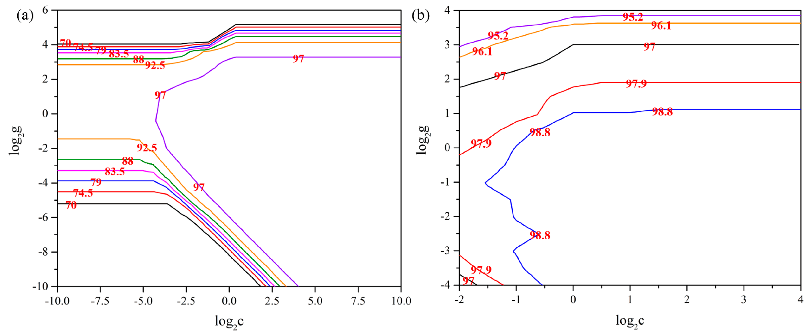
3.2.2. Support Vector Machine

For the SVM model, the radial basis function (RBF) was selected as the kernel function. The penalty parameter (c) and kernel function parameter (g) were optimized. Through the grid search method, in a wide range (2−10–210), we determined that c is 4 and g is 0.047, as shown in Figure 6a. It can be clearly seen that the diagnostic accuracy of the SVM model changed with different c and g values. A further search was needed in a smaller range to get more accurate results. Figure 6b shows the search results in a small range (2−2–24). The best diagnostic results can be acquired from the SVM method at c = 8 and g = 0.062.
This model was used to classify test sets, and the accuracy is shown in Table 2. The average accuracy of the mock-up mural samples is as high as 100%. The average accuracy of an actual mural fragment was only 66.67%; all the spectral data of azurite are completely incorrectly identified. The reason for the unsatisfactory accuracy is that actual murals are seriously affected by surface organic matter, resulting in the uneven strength of trace elements, so the identification accuracy is poor.

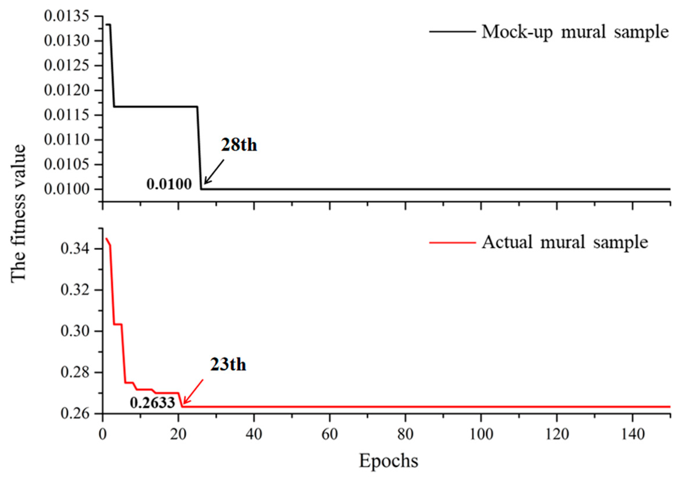
3.2.3. Random Forest

There are two important parameters in RF, one is the number (n) of decision trees, and the other is the number (m) of sample predictors at the tree node. The particle swarm optimization (PSO) algorithm was used to optimize the model. When the particle swarm size was 20, n = 79 and m = 37, the fitness curve was drawn according to the optimal fitness of the training sample obtained from the minimum fitness of each generation, as shown in Figure 7. The curve became stable when the epochs were 28 and 23 in the mock-up mural samples and actual mural fragment. The declining curve represented the effectiveness of the algorithm. Based on the above optimization, the RF prediction model was applied to the test set, and we found that this result of RF was the highest so far, as shown in Table 3.
In the mock-up mural samples, all spectral data were accurately classified, and the average accuracy rate reached 100%, as shown in Table 3. The identification accuracy of three pigments on actual murals reached 83.33%, and the identification results of azurite samples were improved. However, this result still did not meet our expectations because the accuracy of the azurite was unqualified.

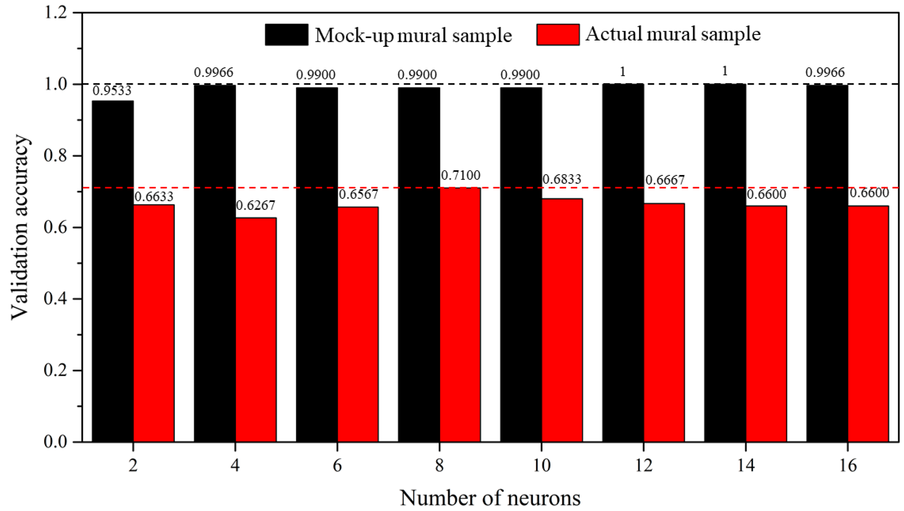
3.2.4. Back Propagation Artificial Neural Network

In the Bp-ANN identification model, the used neural network structure had three layers, which were the input, hidden and output layers. We optimized the number of neurons in the hidden layer, as shown in Figure 8. The results showed that the accuracy of mock-up mural samples corresponding to each neuron is almost the same, but when the number of neurons was eight, the accuracy of the actual mural fragments was the best.
The final prediction results are shown in Table 4. The average accuracy of mock-up mural samples and actual mural fragments was 99.67% and 72.67%, respectively. This result was not as good as the RF model. Only 27 of the 50 spectral data for azurite were accurately identified, and the rest were identified as atacamite. At the same time, the 16 spectra of atacamite were considered to be azurite. The main reason for error identification was the same as the SVM model.

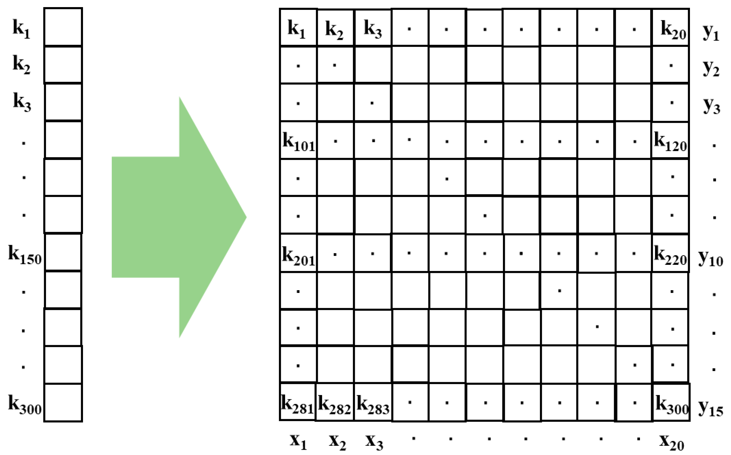
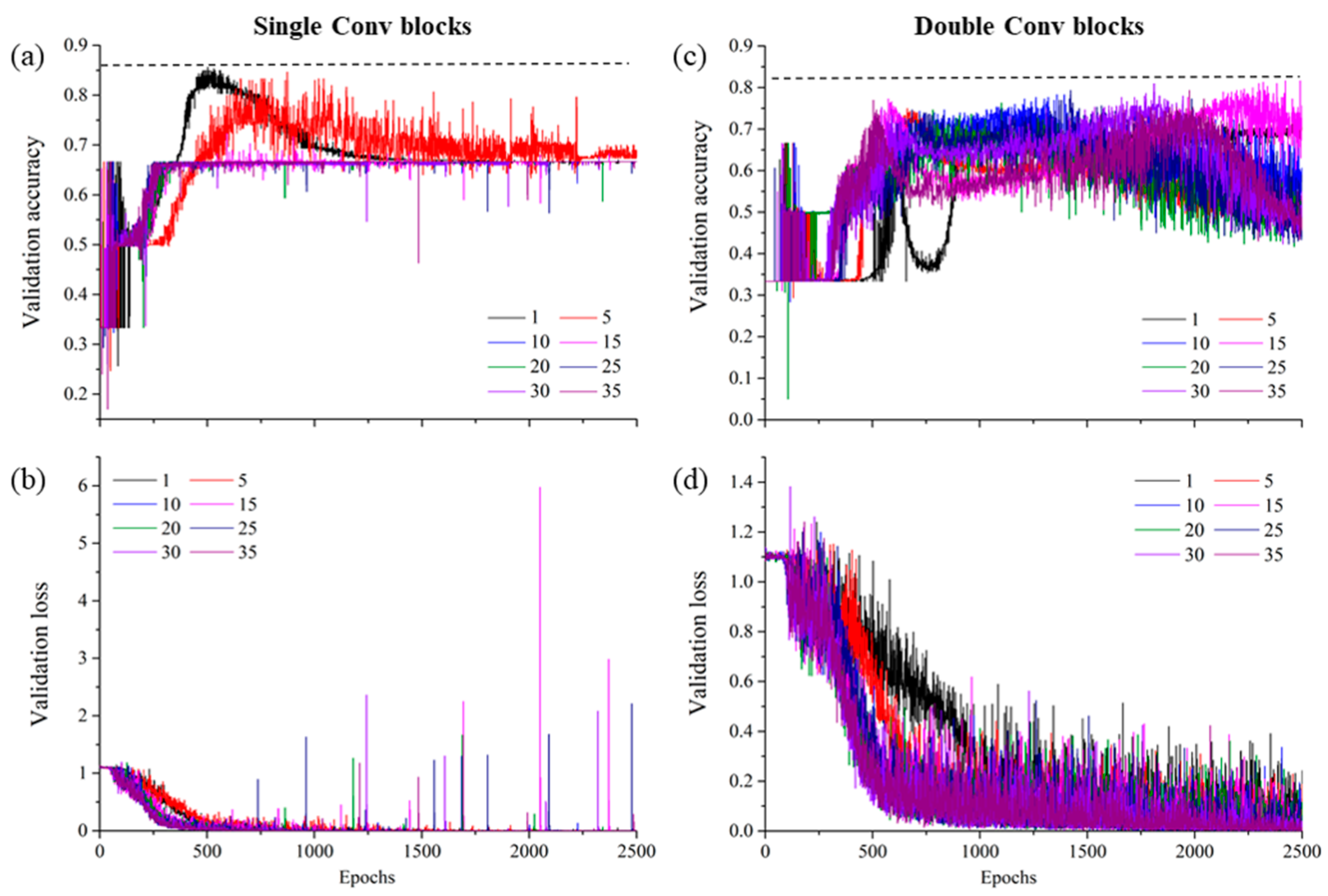
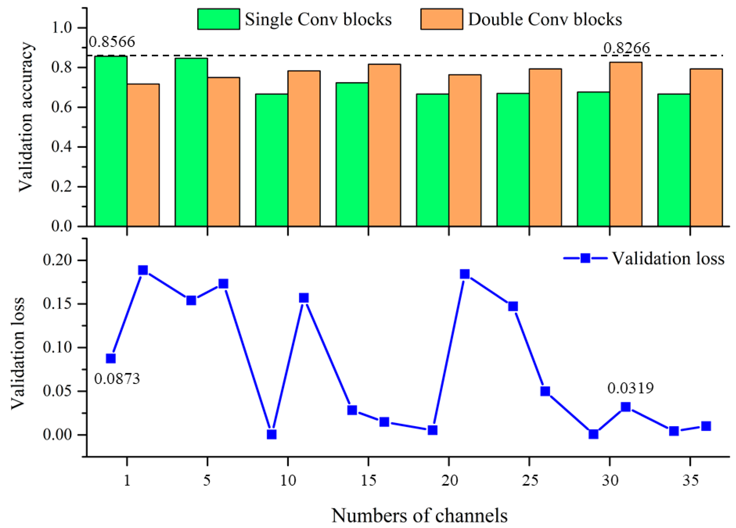
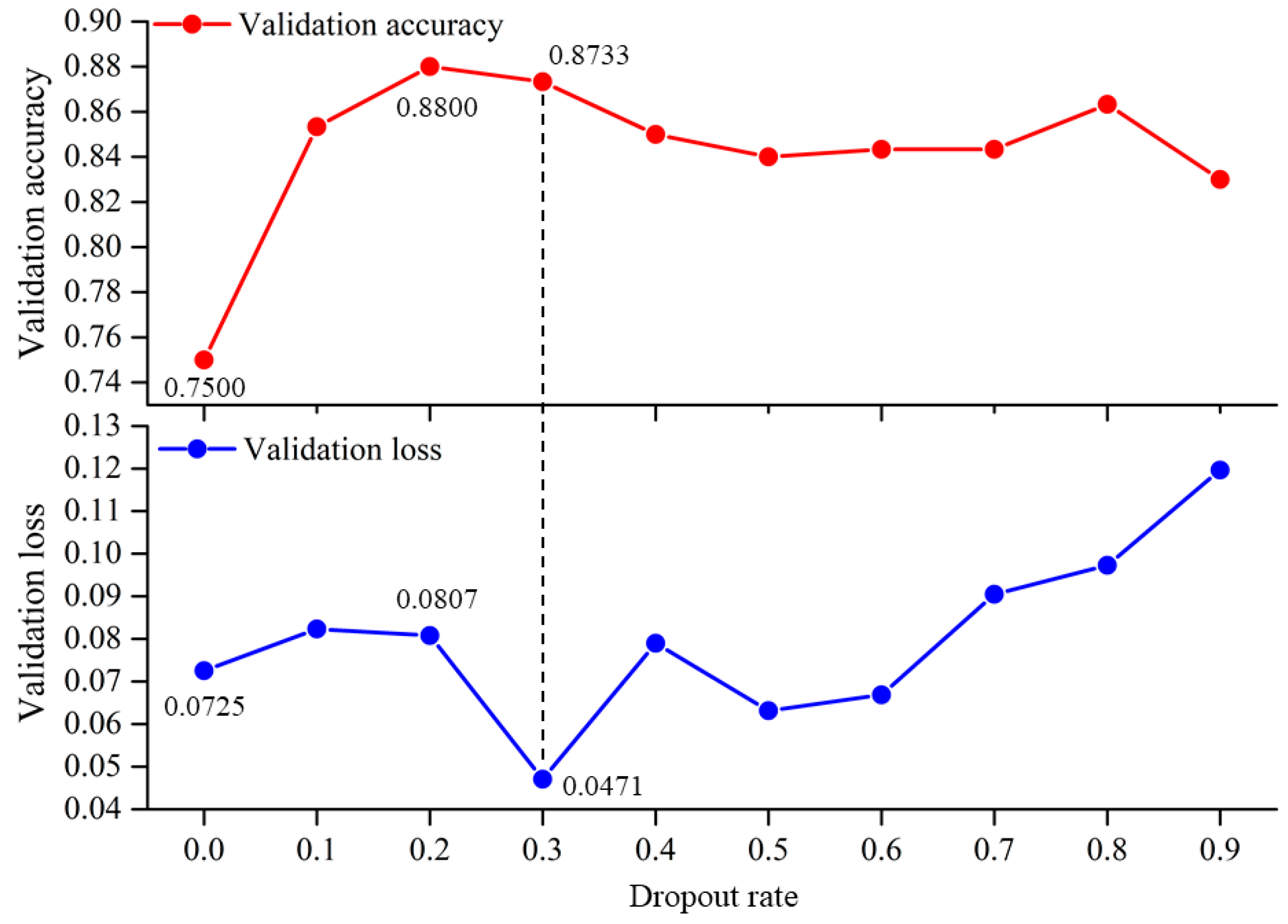
3.3. Two-Dimensional Convolutional Neural Network

Since the input data of 2D-CNN was a matrix, 300 feature peaks needed to be constructed into a matrix of 20 × 15. Figure 9 is the schematic of this process. The data form of the training and test sets were consistent with the above methods, and five-fold cross-validation was still used to ensure the reliability and generalization ability of the calculation results. In the process of constructing the 2D-CNN identification model, we optimized the number of convolution blocks, channels and dropout rate.
Firstly, considering the small amount of data, the single and double convolution blocks with different number channels were selected as the alternative. The batch size was 64, the activation was Sigmoid function, and each training process was terminated after 2500 epochs. It can be seen from Figure 10a that in the case of a single Conv block when the number of channels was one, the accuracy reaches the maximum value with the increase of epoch about 500 times. But due to excessive fitting, the subsequent accuracy was reduced. And the loss value also converges, as shown in Figure 10b. For the double Conv block, in the case of 15 channels, the accuracy was the best when epochs were about 2300, as shown in Figure 10c. The loss value was also reduced to stable, as shown in Figure 10d.
The optimization results are shown in Figure 11. For the single Conv blocks, when the number of channels was one, the accuracy reaches 0.8566, and the loss was reduced by 0.0873. For the double Conv blocks of 15 channels, the accuracy was 0.8266, and the minimum loss was 0.0319. In contrast, the result of a single convolution block with one channel was the best. Hence, the optimized framework of 2D-CNN consisted of a sequential distribution of single Conv blocks with one channel and a fully connected classifier.
To further improve the accuracy, the dropout regularization technique [34] was used to avoid overfitting due to the relatively small amount of data. The validation accuracy with a dropout rate ranging from 0 to 0.9 was compared. As shown in Figure 12, when the dropout rate was 0.3, the validation loss reached the minimum value of 0.0471, a 35.15% decrease compared with the non-regularized model (dropout rate = 0). Meanwhile, the validation accuracy was increased to 0.8733. Although the accuracy was higher when the dropout rate was 0.2, the loss was 11.31% higher than the cost-increasing model. Therefore, the dropout rate in the model was set to 0.3.
The optimized 2D-CNN model was applied to the test set, and the results are shown in Table 5. For the spectra of mock-up mural samples, the average accuracy was 100%. The accuracy of the actual mural fragment data was increased to 94%, among which the wrong samples included three spectra of azurite classified as atacamite, and six spectra of atacamite were classified as azurite. This result has been greatly improved compared with the common machine learning methods.
The identification results of all machine learning methods on the test set under optimal conditions were directly compared, as shown in Figure 13. In addition to the KNN, the accuracy of several methods for mock-up mural samples was relatively average, which can reach about 100%. For actual mural samples, only 2D-CNN can meet the requirements of rapid identification and analysis in Dunhuang Mogao Grottoes.
In 2018, Fan et al. [35] classified 38 mineral pigments using the SAM method, and the result was 94%. Although they used more pigments than we did, they only classified the model samples. For simulated samples, the 2D-CNN model yielded 100%. For real murals with uneven surfaces, the results calculated by the 2D-CNN model were also 100%. Therefore, 2D-CNN was identified as the most suitable identification method for mineral pigment analysis in murals.

4. Conclusions

In this study, LIBS technology combined with a machine learning method was used to accurately identify and classify three mineral pigment samples with Cu as the main element. Firstly, the SelectKBest algorithm was used to screen the spectral characteristics, and 300 characteristic spectral lines with the largest difference among the three pigments were determined to improve the calculation speed by reducing the calculation amount. The identification models of KNN, SVM, RF, Bp-ANN and 2D-CNN were established, and their important parameters were optimized. Including K value, the penalty parameter (c) and kernel function parameter (g), the number of decision trees (n) and the number of sample predictors at the tree node (m), the number of neurons, the number of channels, the number of convolution layers and dropout rate.
The results showed that the accuracy of other models was more than 99% for the mock-up mural samples except for the KNN model. However, for actual mural samples, their accuracy rates were 64.67%, 66.67%, 83.33%, 72.67% and 94%, respectively. Therefore, this study identified the great potential of 2D-CNN in the identification of mural pigments, which can provide a new method for the accurate identification of pigments with similar chemical compositions.

Author Contributions

Writing-review and editing, D.S.; Experimental detection and writing—original draft preparation, Y.Z.; Methodology, Y.Y.; Writing machine learning algorithms, Z.Z. and H.Q.; Sample preparation, Y.W.; Real sample support, Z.Y. and B.S.; Resources, C.D.; Project administration, M.S. All authors have read and agreed to the published version of the manuscript.

Funding

This work was supported by the National Key Research and Development Program of China (No. 2019YFC1520701), the National Natural Science Foundation of China (No. 61965015, 61741513), 2020 Industry Support Plan Project in the University of Gansu Province (No. 2020C-17), Young Teachers Scientific Research Ability Promotion Plan of Northwest Normal University Province (No. NWNW-LKQN2019-1) and Funds for Innovative Fundamental Research Group Project of Gansu Province (No. 21JR7RA131).

Acknowledgments

All authors agree to submit the manuscript to the Chemosensors journal.

Conflicts of Interest

The authors declare no conflict of interest.

References

  1. Fan, J.S. The conservation and management of the Mogao Grottoes. Dunhuang Res. 2000, 63, 1–4. [Google Scholar]
  2. Xu, W.; Sun, C.; Tan, Y.; Gao, L.; Zhang, Y.; Yue, Z.; Shabbir, S.; Wu, M.; Zou, L.; Chen, F.; et al. Total alkali silica classification of rocks with LIBS: Influences of the chemical and physical matrix effects. J. Anal. Atom. Spectrom. 2020, 35, 1641–1653. [Google Scholar] [CrossRef]
  3. Lampakis, D.; Karapanagiotis, I.; Katsibiri, O. Spectroscopic investigation leading to the documentation of three post-byzantine wall paintings. Appl. Spectrosc. 2017, 71, 129–140. [Google Scholar] [CrossRef] [PubMed]
  4. Tomasini, E.P.; Cárcamo, J.; Rodríguez, D.M.C.; Careaga, V.; Gutiérrez, S.; Landa, C.R.; Sepúlveda, M.; Guzman, F.; Pereira, M.; Siracusano, G.; et al. Characterization of pigments and binders in a mural painting from the Andean church of San Andrés de Pachama (northernmost of Chile). Herit. Sci. 2018, 6, 61. [Google Scholar] [CrossRef]
  5. Whittig, L.D.; Allardice, W.R. X-ray diffraction techniques. Methods Soil Anal. Part 1 Phys. Mineral. Methods 1986, 5, 331–362. [Google Scholar]
  6. Bugini, R.; Corti, C.; Folli, L.; Rampazzi, L. Unveiling the use of creta in Roman plasters: Analysis of clay wall paintings from Brixia (Italy). Archaeometry 2017, 59, 84–95. [Google Scholar] [CrossRef]
  7. Uvarov, V.; Popov, I.; Rozenberg, S. X-ray Diffraction and SEM Investigation of Wall Paintings Found in the Roman Temple Complex at Horvat Omrit, Israel. Archaeometry 2015, 57, 773–787. [Google Scholar] [CrossRef]
  8. Robador, M.D.; De Viguerie, L.; Pérez-Rodríguez, J.L.; Rousselière, H.; Walter, P.; Castaing, J. The Structure and Chemical Composition of Wall Paintings from Islamic and Christian Times in the Seville Alcazar. Archaeometry 2016, 58, 255–270. [Google Scholar] [CrossRef]
  9. Realini, M.; Conti, C.; Botteon, A.; Colombo, C.; Matousek, P. Development of a full micro-scale spatially offset Raman spectroscopy prototype as a portable analytical tool. Analyst 2017, 142, 351–355. [Google Scholar] [CrossRef]
  10. Yin, Y.P.; Yu, Z.R.; Sun, D.X.; Shan, Z.; Cui, Q.; Zhang, Y.; Feng, Y.; Shui, B.; Wang, Z.; Yin, Z.; et al. In Situ Study of Cave 98 Murals on Dunhuang Grottoes Using Portable Laser-Induced Breakdown Spectroscopy. Front. Phys.-Lausanne 2022, 10, 94. [Google Scholar] [CrossRef]
  11. Yin, Y.P.; Sun, D.X.; Su, M.G.; Yu, Z.; Su, B.; Shui, B.; Wu, C.; Han, W.; Shan, Z.; Dong, C. Investigation of ancient wall paintings in Mogao Grottoes at Dunhuang using laser-induced breakdown spectroscopy. Opt. Laser Technol. 2019, 120, 105689. [Google Scholar] [CrossRef]
  12. Yin, Y.P.; Sun, D.X.; Yu, Z.R.; Su, M.; Shan, Z.; Su, B.; Dong, C. Influence of particle size distribution of pigments on depth profiling of murals using laser-induced breakdown spectroscopy. J. Cult. Herit. 2021, 47, 109–116. [Google Scholar] [CrossRef]
  13. Gong, T.T.; Tian, Y.; Chen, Q.; Xue, B.; Huang, F.; Wang, L.; Li, Y. Matrix Effect and Quantitative Analysis of Iron Filings with Different Particle Size Based on LIBS. Spectrosc. Spect. Anal. 2020, 40, 7–13. [Google Scholar]
  14. Cao, Z.; An, Y.; Wang, Z.; Guo, L.; Chen, C.A.; Gou, F.; Li, Y. Improved internal standard LIBS method used in CLF-1 exposure to liquid lithium. Nucl. Mater. Energy 2020, 24, 100786. [Google Scholar] [CrossRef]
  15. Yin, W.B.; Zhang, L.; Wang, L.; Li, Z.-X.; Yan, X.-J.; Zhang, Y.-Z.; Jia, S.-T. Research on the Carbon Content of Coal by LIBS. Spectrosc. Spect. Anal. 2012, 32, 55–58. [Google Scholar]
  16. Qi, J.; Zhang, T.L.; Tang, H.S.; Li, H. Rapid classification of archaeological ceramics via laser-induced breakdown spectroscopy coupled with random forest. Spectrochim. Acta B 2018, 149, 288–293. [Google Scholar] [CrossRef]
  17. Duchêne, S.; Detalle, V.; Bruder, R.; Sirven, J.B. Chemometrics and laser induced breakdown spectroscopy (LIBS) analyses for identification of wall paintings pigments. Curr. Anal. Chem. 2010, 6, 60–65. [Google Scholar] [CrossRef]
  18. Bai, X.S.; Syvilay, D.; Wilkie-Chancellier, N.; Texier, A.; Martinez, L.; Serfaty, S.; Martos-Levif, D.; Detalle, V. Influence of ns-laser wavelength in laser-induced breakdown spectroscopy for discrimination of painting techniques. Spectrochim. Acta B 2017, 134, 81–90. [Google Scholar] [CrossRef]
  19. Liu, B.X.; Li, Y.; Li, G.; Liu, A. A Spectral Feature Based Convolutional Neural Network for Classification of Sea Surface Oil Spill. ISPRS Int. J. Geo.-Inf. 2019, 8, 160. [Google Scholar] [CrossRef]
  20. Li, X.L.; He, Z.N.; Liu, F.; Chen, R. Fast Identification of Soybean Seed Varieties Using Laser-Induced Breakdown Spectroscopy Combined with Convolutional Neural Network. Front. Plant Sci. 2021, 12, 714557. [Google Scholar] [CrossRef]
  21. Sang, X.C.; Zhou, R.G.; Li, Y.C.; Xiong, S. One-Dimensional Deep Convolutional Neural Network for Mineral Classification from Raman Spectroscopy. Neural Process. Lett. 2021, 54, 677–690. [Google Scholar] [CrossRef]
  22. Yin, Y.P.; Yu, Z.R.; Sun, D.X.; Su, M.; Wang, Z.; Shan, Z.; Han, W.; Su, B.; Dong, C. A potential method to determine pigment particle size on ancient murals using laser induced breakdown spectroscopy and chemometric analysis. Anal. Methods 2021, 13, 1381–1391. [Google Scholar] [CrossRef] [PubMed]
  23. Mucherino, A.; Papajorgji, P.J.; Pardalos, P.M. K-nearest neighbor classification. In Data Mining in Agriculture; Springer: New York, NY, USA, 2009; pp. 83–106. [Google Scholar]
  24. Buttrey, S.E.; Karo, C. Using k-nearest-neighbor classification in the leaves of a tree. Comput. Stat. Data An. 2002, 40, 27–37. [Google Scholar] [CrossRef]
  25. Képeš, E.; Vrábel, J.; Adamovsky, O.; Střítežská, S.; Modlitbová, P.; Pořízka, P.; Kaiser, J. Interpreting support vector machines applied in laser-induced breakdown spectroscopy. Anal. Chim. Acta 2022, 1192, 339352. [Google Scholar] [CrossRef]
  26. Pisner, D.A.; Schnyer, D.M. Support vector machine. In Machine Learning; Academic Press: Cambridge, MA, USA, 2020; pp. 101–121. [Google Scholar]
  27. Biau, G.; Scornet, E. Rejoinder on: A random forest guided tour. Test 2016, 25, 264–268. [Google Scholar] [CrossRef]
  28. Shi, T.; Horvath, S. Unsupervised Learning with Random Forest Predictors. J. Comput. Graph. Stat. 2006, 15, 118–138. [Google Scholar] [CrossRef]
  29. Li, F.; Lu, A.X.; Wang, J.H.; You, T. Back-propagation neural network–based modelling for soil heavy metal. Int. J. Robot. Autom. 2021, 36, 1–7. [Google Scholar]
  30. Goh, A.T.C. Back-propagation neural networks for modeling complex systems. Artif. Intell. Eng. 1995, 9, 143–151. [Google Scholar] [CrossRef]
  31. Traore, B.B.; Kamsu-Foguem, B.; Tangara, F. Deep convolution neural network for image recognition. Ecol. Inform. 2018, 48, 257–268. [Google Scholar] [CrossRef] [Green Version]
  32. Yang, J.D.; Li, J.P. Application of deep convolution neural network. In Proceedings of the 2017 14th International Computer Conference on Wavelet Active Media Technology and Information Processing (ICCWAMTIP), Chengdu, China, 15–17 December 2017; pp. 229–232. [Google Scholar]
  33. Cormen, T.H.; Leiserson, C.E.; Rivest, R.L.; Stein, C. Introduction to algorithms second edition. In Knuth-Morris-Pratt Algorithm, 2nd ed.; MIT Press and McGraw-Hill: Cambridge, UK, 2001. [Google Scholar]
  34. Hinton, G.E.; Srivastava, N.; Krizhevsky, A.; Sutskever, I.; Salakhutdinov, R.R. Improving neural networks by preventing co-adaptation of feature detectors. arXiv 2012, arXiv:1207.0580. [Google Scholar]
  35. Fan, C.; Zhang, P.C.; Wang, S.; Hu, B.L. A study on classification of mineral pigments based on spectral angle mapper and decision tree. In Tenth International Conference on Digital Image Processing (ICDIP 2018); SPIE: Shanghai, China, 2018; Volume 10806, pp. 1639–1643. [Google Scholar]
Figure 1. (a) Mock-up mural samples in the laboratory, (b) actual mural fragment from the Mogao Grottoes.
Chemosensors 10 00389 g001
Figure 2. Characteristic spectra of three mineral pigments with Cu as the main element.
Chemosensors 10 00389 g002
Figure 3. A schematic depiction of CNN feedforward, (A) convolution layer, (B) pooling layer, (C) fully connected and output layers.
Chemosensors 10 00389 g003
Figure 4. Scores of 300 highest ranked spectral pixels and pixels constituting Cu I 521.81 nm.
Chemosensors 10 00389 g004
Figure 5. Validation accuracy of KNN with different K values.
Chemosensors 10 00389 g005
Figure 6. (a) Large−scale grid search results. (b) Small−scale grid search results.
Chemosensors 10 00389 g006
Figure 7. Variation trend of the fitness value with epoch.
Chemosensors 10 00389 g007
Figure 8. Validation accuracy of Bp-ANN with different numbers of neurons.
Chemosensors 10 00389 g008
Figure 9. A schematic diagram for the conversion of characteristic lines of mineral pigments from one dimension to two dimensions, where ki represents the normalized intensity value of each characteristic line.
Chemosensors 10 00389 g009
Figure 10. (a) The accuracy of Single Conv block corresponding to different channel numbers; (b) The loss of Single Conv block corresponding to different channel numbers; (c) The accuracy of Double Conv block corresponding to different channel numbers; (d) The accuracy of Double Conv block corresponding to different channel numbers. (Lines of different colors represent different channel numbers.).
Chemosensors 10 00389 g010
Figure 11. Validation performance of 2D-CNN with different network structures.
Chemosensors 10 00389 g011
Figure 12. Validation performance of 2D-CNN with different dropout rates.
Chemosensors 10 00389 g012
Figure 13. The accuracy comparison results of all methods for mock-up mural samples and actual mural fragments.
Chemosensors 10 00389 g013
Table 1. Confusion matrix and accuracy of KNN identification model for three samples.
Confusion MatrixIdentification Performance
Sample
Label
Model-Predicted Class
AzuriteMalachiteAtacamiteAccuracy (%)Average (%)
Mock-up sampleAzurite6511246580.33
Malachite2276276
Atacamite00100100
Actual sampleAzurite0050064.67
Malachite247194
Atacamite0050100
Table 2. Confusion matrix and accuracy of SVM identification model for three samples.
Confusion MatrixIdentification Performance
Sample
Label
Model-Predicted Class
AzuriteMalachiteAtacamiteAccuracy (%)Average (%)
Mock-up sampleAzurite10000100100
Malachite01000100
Atacamite00100100
Actual sampleAzurite0050066.67
Malachite0500100
Atacamite0050100
Table 3. Confusion matrix and accuracy of RF identification model for three samples.
Confusion MatrixIdentification Performance
Sample
Label
Model-Predicted Class
AzuriteMalachiteAtacamiteAccuracy (%)Average (%)
Mock-up sampleAzurite10000100100
Malachite01000100
Atacamite00100100
Actual sampleAzurite41098283.33
Malachite047394
Atacamite1303774
Table 4. Confusion matrix and accuracy of Bp-ANN identification model for three samples.
Confusion MatrixIdentification Performance
Sample
Label
Model-Predicted Class
AzuriteMalachiteAtacamiteAccuracy (%)Average (%)
Mock-up sampleAzurite1000010099.67
Malachite199099
Atacamite00100100
Actual sampleAzurite270235472.67
Malachite048296
Atacamite1603468
Table 5. Confusion matrix and accuracy of 2D-CNN identification model for three samples.
Confusion MatrixIdentification Performance
Sample
Label
Model-Predicted Class
AzuriteMalachiteAtacamiteAccuracy (%)Average (%)
Mock-up sampleAzurite10000100100
Malachite01000100
Atacamite00100100
Actual sampleAzurite47039494
Malachite0500100
Atacamite604488
Publisher’s Note: MDPI stays neutral with regard to jurisdictional claims in published maps and institutional affiliations.

