Assessment of Optimization Methods for Aeroacoustic Prediction of Trailing-Edge Interaction Noise in Axisymmetric Jets

Abstract

Our concern in this paper is in the fine-tuning of the arbitrary parameters within the upstream turbulence structure for the acoustic spectrum of a rapid-distortion theory (RDT)-based model of trailing-edge noise. RDT models are based on an appropriate asymptotic limit of the Linearized Euler Equations and apply when the interaction time of the turbulence with the surface edge discontinuity is small compared to the eddy turnover time. When an arbitrary transversely sheared jet mean flow convects a finite region of nonhomogeneous turbulence, the acoustic spectrum of the pressure field scattered by the trailing-edge depends on (among other things) the upstream turbulence via the Fourier transform of the correlation function, $R_{22}$ (where subscript 2 refers to a co-ordinate surface normal to the plate). We show that the length and time scale parameters that govern the spatial and temporal de-correlation of $R_{22}$ can be found using formal optimization methods to avoid any uncertainty in their selection by hand-tuning. We assess various optimization methods that are broadly categorized into an ‘evolutionary’ and ‘non-evolutionary’ paradigm. That is, we optimize the acoustic spectrum using the Multi-Start algorithm, Particle Swarm Optimization and the Multi-Population Adaptive Inflationary Differential Evolution Algorithm. The optimization is based upon different objective functions for the acoustic spectrum and/or turbulence structure. We show that this approach, while resulting in the total modest increase in computation time (on average 2 h), gives excellent prediction over most frequencies (within 2–4 dB) where the trailing-edge noise associated amplification in sound exists.

1. Introduction

The advent of the jet engine in the mid-twentieth century [1] brought with it the intrusion caused by aircraft noise to the communities living near airports. In its entirety, however, the aircraft noise problem is an incredibly complex one [2]. For example, Dobrzynski [3] shows that the radiated sound on approach for both short and long stage length aircraft is evenly split between the engine and the airframe. Engine associated noise is generated from the internal moving surfaces within the engine components as well as from the exhaust gas emanating at the nozzle exit. The breakdown of the latter results in both jet noise and jet-surface interaction noise components when the turbulent air interacts with the airframe, wing edges and other external surfaces.

The trailing-edge component is a particularly dangerous noise source owing to the large increase in low frequency sound when the observation point is above or below the plate surface and vertical location $\left(h\right)$ of the trailing-edge is of the order of jet diameter, $h\sim D$. Experiments on edge noise began in the 1970s by Olsen & Boldman [4] (discussed below). In the early 1980’s, Wang [5] showed that the presence of an external surface increased the noise measured on the same side as the jet flow in comparison to the isolated jet. This amplification of sound due to the interaction with the trailing-edge is mainly at low frequencies up to the peak Strouhal number (i.e., the normalized angular frequency, $St=fD/U_j$ based on jet exit velocity, $U_j$ and diameter, D); typically this is at $St\sim 0.1$. It also dominates at larger observation angles $\theta$ to the jet axis [6,7]. Bridges’ recent experiments [8] confirm the work done in the 1970s by Olsen & Boldman [4] and Wang’s result by showing that the amplification in sound perpendicular to the jet axis (i.e., $\theta ={90}^{\circ }$) is typically of the order of 10 dB for a high speed jet at an acoustic Mach number based on the speed of sound at infinity, $Ma=U/c_{\infty }$, of $Ma=0.9$. As $\left(\theta \right)$ reduces, the jet noise contribution increases until, at shallow angles (e.g., $\theta ={30}^{\circ }$), the latter jet noise dominates the total noise radiation signature at almost all measured frequencies; typically this covers Strouhal numbers, $St=[0.01,2.0]$. The Bridges’ [8] and Bridges et al. [9] datasets also covered the parameter range of acoustic Mach number, $Ma$, edge location with respect to the nozzle lower lip line and the nozzle shape itself. We briefly summarize these trends now. (1). The amplification in sound is greater at lower $Ma$, e.g., at $Ma=0.5$ cf. $0.9$; this is consistent with the ‘dipole’ directionality of the edge noise source. (2). As the vertical standoff distance, $h/D$, is increased the edge noise reduces in magnitude. At the limiting condition where $h\gg D$, the amplification in sound due to the edge vanishes and the total sound owes itself to the jet noise alone. The streamwise location also has an important impact on the magnitude of low frequency noise amplification. Bridges’ results show that the edge must be placed in the vicinity of where the jet potential core terminates for the amplification to reach its greatest magnitude. (3). The round jet appears to result in greater noise amplification than the high-aspect ratio rectangular (i.e., planar) jet flow [9].

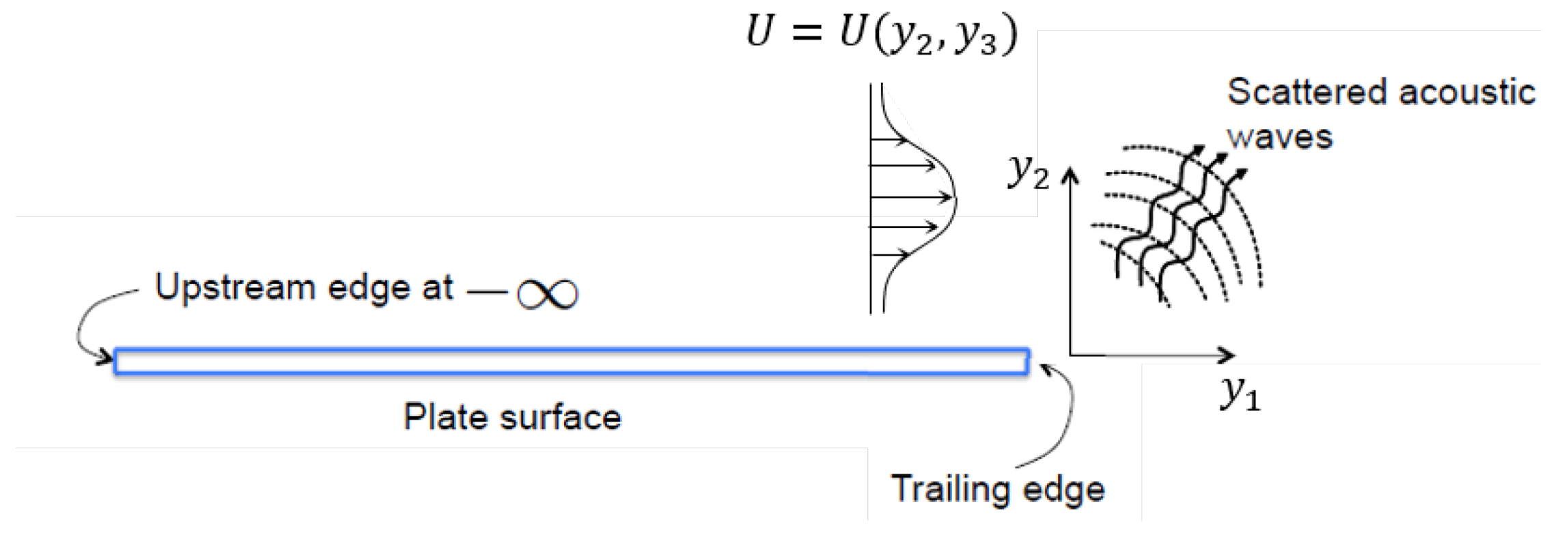
From an analytical and numerical standpoint, a lot of work has been done on this problem [10,11,12,13,14,15]. The discontinuity in the solid surface boundary condition can be treated formally using the Wiener-Hopf technique for a flat plate that is doubly infinite in the spanwise direction and lies parallel to the level curves of the streamwise mean flow. See Figure 1 for a depiction of this problem in the $(y_1-y_2)$ plane. The so-called ‘gust solution’ then acts as the input to an inhomogeneous boundary value problem in which the scattered pressure field is determined at the output. Goldstein et al. [10,11,12] used the method of matched asymptotic expansions at the low frequency limit to construct the gust-induced boundary condition and the homogeneous solutions to the Rayleigh equation that enter in the solution to the Wiener-Hopf problem for the acoustic field scattered by the edge. This solution (Equations (6.26) and (6.27) in [12]) was analytically continued to high frequencies, and (Equations (6.28)–(6.30)) show that the mean square scattered pressure depends on the upstream structure of the two-point time-delayed turbulence correlation $R_{22}$ where the subscript 2 denotes the co-ordinate plane normal the plate surface. Just as in acoustic analogy models of jet noise [16,17], the correlation function is modeled by comparing to a wide bank of experimental data (see, e.g., ref. [18]) on jet flow turbulence.

All models are formulated with arbitrary ’tuning’ parameters to quantify the degree of spatial and temporal de-correlation as well as the permanence of a finite anti-correlation region in spatial and temporal separation [14]. Previous modeling approaches tuned these scales by hand to obtain good agreement with the acoustic data. In this paper we show that this form of empiricism can be avoided entirely by using an appropriate numerical optimization routine to determine the parameters for an objective function that seeks to minimize the difference between the functional form of the turbulence model and turbulence data as well as minimizing the difference between acoustic predictions and acoustic data.

A (single-objective) optimization problem can be described in terms of minimizing the objective function $J(\mathit{x},\mathit{\psi })$, where $x_i(i=1,n)$ are the n design variables which are modified to find the optimum, and $\mathit{\psi }$ are the state parameters which describe the system [19]. The objective function may also be subject to (in general) a total $(m,p)$ of (inequality/equality) constraints that take the form:

$$\begin{array}{cc}\hfill & g_j\left(\mathit{x}\right)\le 0j=1,m\hfill \\ \hfill & h_k\left(\mathit{x}\right)=0k=1,p\hfill \end{array}$$

(1)

Additionally, the design variables may be bounded $(x_{i,\mathrm{LOWER}}\le x_i\le x_{i,\mathrm{UPPER}},i=1,n)$, which are known as side constraints.

Optimization algorithms can find multiple solutions to this problem which are known as local optima. Hence, the algorithms can be split into two categories: local optimization methods (which find the local minimum for the starting conditions) and global optimization methods (which aim to find the global minimum of the search space). The majority of local methods use gradient information to find the optimum and there are several methods to do this [20,21,22,23]. However if the problem has multiple local minima, these gradient methods will converge to the closest minimum not necessarily the global. Each minimum has a basin of attraction, where a design point initialised within the basin converges to that local minimum. Hence, local optimization strongly depends on the location of the initial design point. Global optimization methods aim to find the global optimum, however, it should be noted that it cannot be guaranteed that the global optimum will be found, only that it would be if the algorithm could run indefinitely. Global optimization can be split into three types of algorithm: Multi-Start algorithms, evolutionary algorithms and deterministic algorithms. Multi-Start algorithms perform local optimizations at different starting locations, and choose the best local optimum to be the global optimum. Evolutionary algorithms are stochastic and heuristic, they advance a population of design parameters through the search space to find the global optimum. Deterministic algorithms typically require manipulation of the objective function and are designed to solve specific classes of problem [24], an overview of these is described in [25], and will not be further discussed here.

Optimization methods have been used for this kind of problem in aeroacoustics before, for example the Multipoint Approximation Method (MAM) [26,27,28]. This method was designed for computationally expensive and noisy objective functions, so it uses trust regions and a series of approximations to the objective function. It is similar to the Multi-Start algorithm in that it uses multiple starting locations, however it differs by approximating the objective function. In this paper, the objective function is not computationally expensive, therefore we investigate the Multi-Start method instead.

The rest of the paper is organized as follows. In Section 2 we summarize the general theory to determine the acoustic field scattered by the trailing-edge and show the final formula that we use for the subsequent optimization experiments that we perform in order to fine tune the modeling of the correlation function $R_{22}$. Section 3 then reviews the various types of optimization that can be used for problems of this type paying particular attention to evolutionary algorithms. Popular evolutionary algorithms include the Genetic Algorithm (GA) [29] which was inspired by Darwin’s principle of survival of the fittest, Particle Swarm Optimization (PSO) [30] which is based on a social model and differential evolution (DE) [31].

Specifically, we discuss the advantages and disadvantages of three methods (the non-evolutionary Multi-Start [32,33,34], and the evolutionary algorithms: Particle Swarm Optimization (PSO) [30] and Multi-Population Adaptive Inflationary Differential Evolution Algorithm (MP-AIDEA) [35] which is an extension to the original differential evolution algorithm) for a problem of this type and the results that are obtained for the parameters under different objective functions for the turbulence and/or final acoustic predictions (i.e., when comparison is made to turbulence and/or acoustic data). Finally in Section 4 we conclude by discussing the applicability of using such optimization approaches in acoustic modeling problems.

2. Summary of the Mathematical Modeling of Trailing-Edge Noise and Defining the Objective Functions

Rapid-distortion theory (RDT) analyzes the changes in turbulent flows by using linearized equations. It is, therefore, ideally suited to analyze the rapid changes that occur when a turbulent flow interacts with a discontinuity at the boundary of a solid surface embedded in the flow. It applies whenever the turbulence intensity is small and the length (or time) scale over which the changes take place is short compared to the length (or time) scale over which the turbulent eddies evolve. These assumptions imply, among other things, that the resulting flow is inviscid and non-heat conducting and is, therefore, governed by the Linearized Euler Equations, i.e., the Euler equations linearized about an arbitrary, usually steady, solution (the base flow) to the nonlinear equations. Goldstein et al. [11] showed that the upstream boundary conditions can be imposed infinitely far upstream in a region where the flow is undisturbed by the interaction.

Goldstein et al. [12] used rapid distortion theory to determine the trailing-edge noise spectrum above the flat plate (given the Fourier transform of the mean square scattered pressure ${\left[p^{\prime s}(\mathit{x},t)\right]}^2$), denoted by $I(\mathit{x},\omega )$ for the axisymmetric jet $U\left({\mathit{y}}_T\right)$ interacting with the flat plate as depicted in Figure 1, and is given by (Equations (6.26) and (6.27) in their paper):

$$\begin{array}{c}\hfill I(\mathit{x},\omega )\to {\left(\frac{k_{\infty }}{4\pi |\overline{\mathit{x}}|}\right)}^2\underset{-\infty }{\overset{0}{\int }}\underset{-\infty }{\overset{0}{\int }}D(u,\tilde{u};\theta )\overline{S}(u,\tilde{u};\omega )dud\tilde{u},\end{array}$$

(2)

where $D(u,\tilde{u};\theta )$ is the round jet directivity factor determined by application of the Wiener-Hopf technique (i.e., Equation (13) in Afsar et al. [13]), ${\mathit{y}}_T=(y_2,y_3)$ are transverse co-ordinates and,

$$\begin{array}{c}\hfill \overline{S}(u,\tilde{u};\omega )={\left({\rho }_{\infty }{c}_{\infty }^2\right)}^2\underset{-\pi }{\overset{\pi }{\int }}\underset{-\pi }{\overset{\pi }{\int }}S(u,\tilde{u}|v,\tilde{v};\omega ){\left|\frac{dz}{dW}\right|}^2{\left|\frac{d\tilde{z}}{d\tilde{W}}\right|}^{2}dvd\tilde{v}.\end{array}$$

(3)

The function $S(u,\tilde{u}|v,\tilde{v};\omega )$ derived in [12] is

$$S(u,\tilde{u}|v,\tilde{v};\omega )=\left[\frac{dU/du}{U^2\left(u\right)}\frac{dU/d\tilde{u}}{U^2\left(\tilde{u}\right)}\nabla u\tilde{\nabla }\tilde{u}{\omega }^2\right]F(u,\tilde{u},v,\tilde{v})$$

(4)

This result shows, among other things, that $S(u,\tilde{u}|v,\tilde{v};\omega )$ is directly proportional to the Fourier transform of the streamwise-independent turbulence statistical quantity, ${\widehat{R}}_{22}(\tilde{u}-u,\tilde{v}-v;\omega )$ which represents the Fourier transform of the two-point time delayed correlation function of the transverse velocity normal to the plate surface at $u=0$ (see Afsar et al. [13]).

Our starting point is, however, a spectral function $F(u,\tilde{u},v,\tilde{v})$ which is slightly more general than that used in [12] (Equation (4.22) in their paper). Since correlation functions of the type $R_{22}$ will anti-correlate (i.e., become negative) for some values of its arguments [13], including such effects means that a mathematical model for $R_{22}$ must have additional algebraic behaviour, for example given by the $a_1$ term in the following formula

$$R_{22}\left(\tau \right)\sim (1-a_1\tau )e^{-\tau },$$

(5)

where $\tau$ is the time-delay between the two space-time points being correlated far upstream of the interaction region near the trailing edge as required by the theory in [11]. Hence, the spectral function, $F(u,\tilde{u},v,\tilde{v})$, from Equation (4) is given by the following formula:

$$\begin{array}{cc}\hfill F(u,\tilde{u},v,\tilde{v})=& l_2^{4}A(u,\tilde{u})[(1-a_1)\frac{{\tau }_{0}f}{\pi \sqrt{1+{\tilde{\omega }}^2}}{K}_1(f\sqrt{1+{\tilde{\omega }}^2})+\frac{a_1{\tau }_0{f}^2{\tilde{\omega }}^2}{\pi (1+{\tilde{\omega }}^2)}\hfill \\ \hfill & [\frac{1}{2}(K_0(f\sqrt{1+{\tilde{\omega }}^2})+K_2(f\sqrt{1+{\tilde{\omega }}^2}))+\frac{K_1(f\sqrt{1+{\tilde{\omega }}^2})}{f\sqrt{1+{\tilde{\omega }}^2}}]],\hfill \end{array}$$

(6)

where $K_0,K_1,$ and $K_2$ are the modified Bessel functions of the second kind of order $0,1,$ and 2 respectively, $A(u,\tilde{u})$ is the amplitude function and $f=|(\tilde{u}-u)/l_2+(\tilde{v}-v)/l_3|$ controls the $(u,v)$ de-correlation via the parameters $(l_2,l_3)$.

The objective functions are then defined as the mean squared error between the acoustic/turbulence models (Equations (2) and (5)) and the relevant experimental data [36,37] is given by the following optimization norms:

$$\begin{array}{cc}\hfill J_A(\mathit{x},\mathit{\psi })& =\frac{1}{N_A}\sum _{i=1}^{N_A}{(I(\mathit{x},{\omega }_i,\mathit{\psi })-E_A(\mathit{x},{\omega }_i,\mathit{\psi }))}^2\hfill \\ \hfill J_R(\mathit{x},\mathit{\psi })& =\frac{1}{N_R}\sum _{i=1}^{N_R}{(R_{22}(\mathit{x},{\tau }_i,\mathit{\psi })-E_R(\mathit{x},{\tau }_i,\mathit{\psi }))}^2,\hfill \end{array}$$

(7)

where: $N_A,N_R$ is the number of experimental data points we are optimizing against for acoustics and $R_{22}$ respectively, $I(\mathit{x},{\omega }_i,\mathit{\psi })$ is the acoustic spectrum result using the model for the ith frequency ${\omega }_i$, and $E_A(\mathit{x},{\omega }_i,\mathit{\psi })$ is the corresponding experimental data. Likewise $R_{22}(\mathit{x},{\tau }_i,\mathit{\psi })$ is the result using our turbulence model at the ith time delay ${\tau }_i$, and $E_R$ is the corresponding experimental data.

The vector of state parameters ($\mathit{\psi }$) is the minimum set of parameters which describe the system and how it responds to input [19]. Our problem can be thought of as an “input/output system” where an input turbulence spectrum interacts with the streamwise discontinuity at the trailing-edge and produces noise. The sound radiation will depend on the acoustic Mach number of the jet ($Ma$), and the location where the noise measurements take place (far field angle, $\theta$, measured with respect to the jet axis and azimuthal angle, $\varphi$). On the other hand the turbulence correlation function, $R_{22}$, is independent of these parameters, and instead depends on the location where the turbulence is measured ($y_1/D,r/D$), where $y_1/D$ is the streamwise location from the nozzle exit normalized by the nozzle diameter and $r/D$ is the radial location from the jet centerline ($r^2=y_2^2+y_3^2$). The experimental set-up can be found in several papers [11,12,37].

The $\mathcal{O}\left(1\right)$ parameters $(a_1,l_2,l_3,{\tau }_0)$ in the spectral function $F(u,\tilde{u},v,\tilde{v})$ are selected in order to find the optimum acoustic spectrum predictions across acoustic Mach number $\left(Ma\right)$ and far-field angle $\theta$, whilst maintaining a physically admissible turbulence structure. In the following sections we discuss the different optimization methods that can be used to achieve this. Since it was found that there were multiple local minima, only global optimization routines were considered. The location of the trailing edge $(x_{TE}/D,y/D)$ in all of the numerical tests investigated below is taken to be the same as Goldstein et al. [12] (see their Figure 4). In the following sections of this paper, the acoustic spectrum $I(\mathit{x},\omega )$ is calculated in the form of the power spectral density of the far-field pressure fluctuation versus Strouhal number, which is defined in this case as $St=fh/U$, and is presented in the usual dB scale where $PSD=10log(4\pi I(\mathit{x},\omega )U/h{p}_{\mathrm{ref}}^2)$ (relative to $p_{\mathrm{ref}}=20 \mathsf{\mu }\mathrm{Pa}$). We show results only at the observation point of $\theta ={90}^{\circ }$ where the trailing edge noise is largest [36] to illustrate the benefit of optimization.

3. Evolutionary Versus Non-Evolutionary Optimization Methods

The non-evolutionary Multi-Start method is the most straightforward global optimization routine. It follows on from local optimization in that it simply performs a local optimization algorithm at several different starting points within the design space [32,33,34]. The local optima can then be compared to find the global optimum. As the number of starting points increase, the probability of finding the global optimum also increase. Often, a Design of Experiments (DOE) is performed prior to Multi-Start to initialise design points within known basins.

Evolutionary algorithms are specifically designed to work on black box problems, i.e., they do not need direct access to the inner workings of the objective function nor do they need gradient information. Consequently, they can be used for non-smooth functions and it is not required that the programmer knows anything about the structure of the objective function. Evolutionary algorithms are known to be robust and have a good chance of finding the global optimum since they advance a fixed population of design variables through the search space. However, they are computationally expensive and require the tuning of parameters to solve each problem [24]. There are several types of evolutionary algorithm, two of the most popular are Particle Swarm Optimization (PSO) and Differential Evolution (DE).

Particle Swarm Optimization (PSO) [30] was developed from a social model. Each particle utilizes not only its own past experience to find an optimum but also that of the group at large. It involves initializing the population and a velocity vector for each particle. The velocity vector is then updated by including information from the particles past and from the group. More recently there have been modifications to PSO to better handle optimization problems with constraints [38]. There are three parameters which need to be tuned for the specific optimization problem. These are, the inertia parameter w, and the trust parameters $c_1,c_2$. The choices of parameters are very important and some recommendations are given in [39]. This paper uses the default parameters given in Matlab which adapts the inertia weight within bounds ($0.1\le w\le 1.1$) and uses the trust parameters ($c_1=c_2=1.49$).

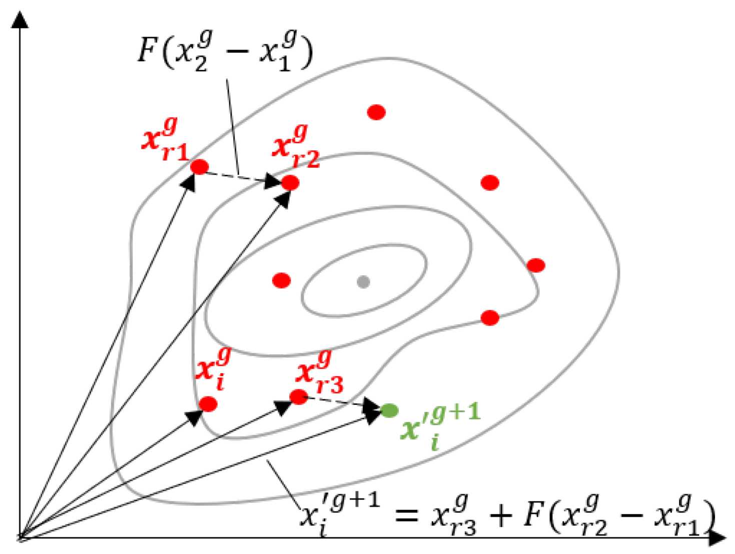
Differential Evolution (DE) [31] also initializes a population of design points and then utilizes information from these points to mutate and find the next generation of design points. There are several different methods of differential evolution but the ‘classic’ method (DE/rand/1/bin) mutates the design parameters through the equation: $x_i^{{}^{\prime }g+1}=x_{r_1}^g+F(x_{r_2}^g-x_{r_3}^g)$ where g is the current generation, i is the individual in the population, and ($r_1,r_2,r_3\ne i$) are random parents in the population. The parameter F is the differential weight and controls the amplification of the differential, it typically lies within the interval 0.4–1 [40]. The mutation is demonstrated in Figure 2 for two dimensions.

Following mutation, crossover is used to increase the diversity of the population, after which the parent and child designs are compared and the best is selected to be the design point for the next generation. The second parameter of differential evolution is the crossover ratio: $0<CR<1$, this and the differential weight, F, need to be selected by the programmer.

There are several variations of the evolutionary algorithms which make them more complex and robust. An extension of the differential evolution algorithm, which we use in this paper, is the Multi-Population Adaptive Inflationary Differential Evolution Algorithm (MP-AIDEA) [35]. This uses multiple populations and combines basic differential evolution with monotonic basin hopping (MBH) to reduce the risk of converging to a minimum which is not global, it also adapts the optimization parameters autonomously. It is a further advancement on the inflationary differential evolution algorithm (IDEA) which only uses a single population and requires the parameters to be chosen by the programmer [41].

When a minimum has been found the monotonic basin hopping (MBH) [42] method generates a new point within the neighbourhood of this minimum (where the neighbourhood is defined as $2\Delta$). A local search is performed from this point and if the minimum found is better than the previous one it is chosen and a new point generated in its neighbourhood, and so on. If no better points are found for $n_{samples}$ then a restart can be performed.

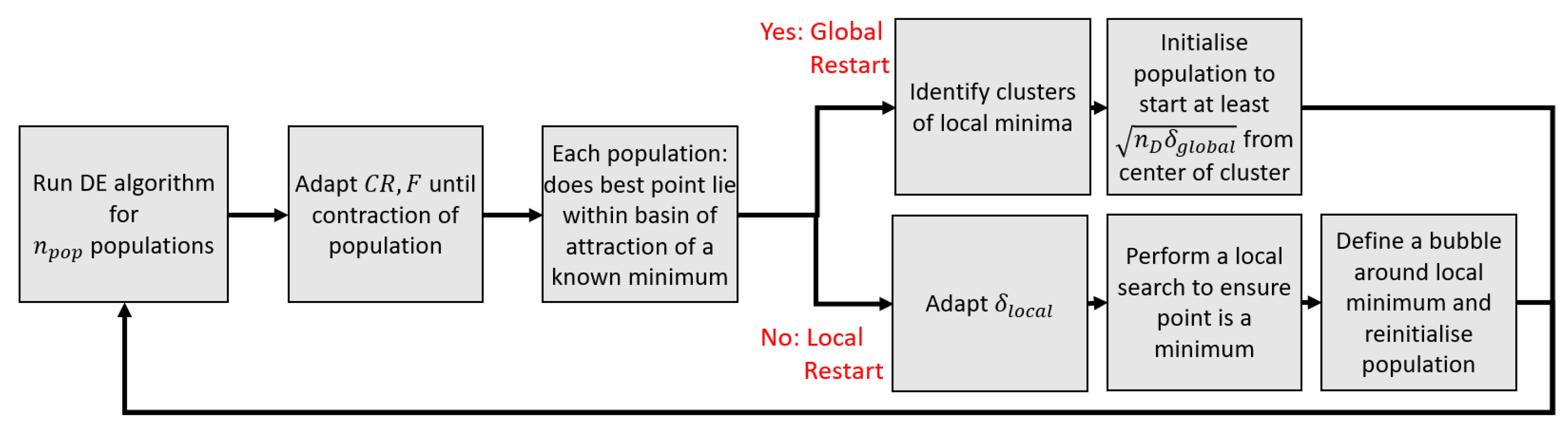
IDEA uses MBH when the population contracts within a radius defined as the contraction limit (a parameter to be defined), when the population reaches this limit it is unlikely to be able to escape and search elsewhere in the design space, hence the need for a restart. Instead of using a local search within MBH it uses differential evolution. MP-AIDEA adapted IDEA to adjust the main parameters (crossover probability $CR$, differential weight F, local restart bubble ${\delta }_{local}$, and the number of local restarts $n_{LR}$) autonomously. This makes the algorithm easier to apply to different problems. For full details of the algorithm refer to [35]. To adapt the values of ${\delta }_{local}$ and $n_{LR}$ the restart of the population needs to be evaluated, therefore, multiple populations are used and evolved in parallel. The parameter $n_{LR}$ is removed in this algorithm and a procedure to decide whether a local or global restart should be run is implemented instead. Figure 3 demonstrates the algorithm.

4. Possible Routes to Minimizing the Objective Function in Equation (7)

There are various approaches to determine the parameters in the spectral function $F(u,\tilde{u},v,\tilde{v})$. One way is by hand as in [12], but here we use the following methods:

• Method 1: Optimize the acoustic model to find the 4 parameters.
• Method 2: Optimize the $R_{22}$ model to find $a_1$ and hand-tune the other 3 parameters for acoustic predictions.
• Method 3: Optimize the $R_{22}$ model to find $a_1$, and optimize the acoustic model to find the other 3 parameters.

Table 1. Optimization problem statement for each method (hyphens indicate that no optimization was carried out).

	Method 1		Method 2		Method 3
	Acoustics	${\mathit{R}}_{22}$	Acoustics	${\mathit{R}}_{22}$	Acoustics	${\mathit{R}}_{22}$
Objective function	$J_A(\mathit{x},\mathit{\psi })=0$	-	-	$J_R(\mathit{x},\mathit{\psi })=0$	$J_A(\mathit{x},\mathit{\psi })=0$	$J_R(\mathit{x},\mathit{\psi })=0$
State parameters ($\mathit{\psi }$)	$Ma,\theta ,\varphi$	-	-	$x/D,y/D$	$Ma,\theta ,\varphi$	$x/D,y/D$
Design parameters ($\mathit{x}$)	$a_1,l_2,l_3,{\tau }_0$	-	-	$a_1$	$l_2,l_3,{\tau }_0$	$a_1$
Constraints	$g_1$	-	-	$g_2$	$g_3$	$g_2$

sets out the optimization problem which is to be solved for each method, where the objective functions $J_A,J_R$ were defined in Equation (7).

There are no equality or inequality constraints for this problem, only side constraints which were chosen to be:

$$\begin{array}{cc}\hfill g_1:& 0<a_1<1, 0<l_2<5, 1<l_3<10, 1<{\tau }_0<10\hfill \\ \hfill g_2:& 0<a_1<1\hfill \\ \hfill g_3:& 0<l_2<5, 1<l_3<10, 1<{\tau }_0<10\hfill \end{array}$$

(8)

The acoustic spectrum results using these methods will be compared to experimental results from [37] for three acoustic Mach numbers $Ma=0.5,0.7,0.9$ above the plate ($\varphi =90$), and at the far field angle ($\theta =90$) where jet surface interaction is greatest.

We also compare the $R_{22}$ model using the values found for $a_1$ against experimental data from Bridges [36] at the end of the potential core on the shear layer ($y_1/D=6,r/D=0.5$).

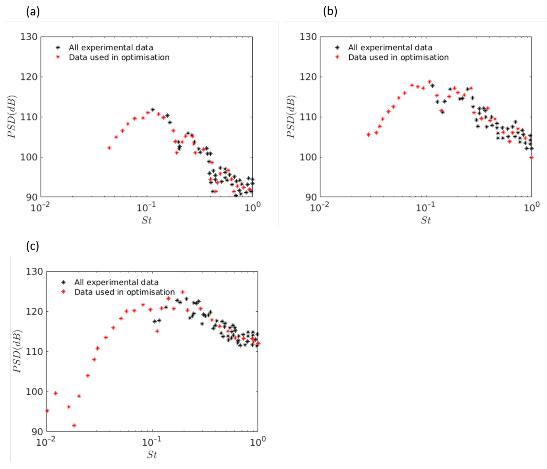
To reduce the time taken in optimization, for each acoustic Mach number 30 points were chosen from the experimental acoustic data (see Figure 4). The acoustic model was then run for each of these points to calculate the objective function.

We compare the results from three optimization routines: The Multi-Population Adaptive Inflationary Differential Evolution Algorithm (MP-AIDEA), Particle Swarm Optimization (PSO), and Multi-Start. The Multi-Start and PSO optimizations were done using the in-built Matlab routines. Multi-Start was carried out using 500 starting points.

5. Results

Since the optimization routines are stochastic, they were ran several times for $Ma=0.9,\theta =90$ to see if they consistently converged. Figure 5 shows the variance of parameters found using Particle Swarm Optimization. Likewise, Figure 6 and Figure 7 show the variance of parameters for MP-AIDEA and Multi-Start respectively. The range of objective function values corresponding to these parameters obtained from each routine are shown in Figure 8.

Table 2. Ma = 0.5, $\theta =90$: Comparison of parameters found from the optimization methods.

Ma = 0.5, $\theta =90$
	Method 1			Method 2	Method 3
	MP-AIDEA	Multi-Start	PSO	Hand-Tuned	MP-AIDEA	Multi-Start	PSO
$a_1$	0.01	0.10	0.00	0.85	0.85	0.85	0.85
$l_2$	2.52	2.18	2.57	1.30	1.51	1.30	1.49
$l_3$	1.01	1.01	1.00	5.00	1.00	2.50	1.00
${\tau }_0$	2.61	2.04	2.69	5.00	3.68	3.52	3.54
fval	14.29	15.47	14.24	20.75	15.68	17.90	15.66
Time (s)	9538	6044	7766	-	7098	4700	7507

,

Table 3. Ma = 0.7, $\theta =90$: Comparison of parameters found from the optimization methods.

Ma = 0.7, $\theta =90$
	Method 1			Method 2	Method 3
	MP-AIDEA	Multi-Start	PSO	Hand-Tuned	MP-AIDEA	Multi-Start	PSO
$a_1$	0.59	0.56	0.60	0.85	0.85	0.85	0.85
$l_2$	1.39	1.14	1.37	0.90	1.05	0.89	1.06
$l_3$	1.02	3.22	1.00	5.00	1.00	2.80	1.00
${\tau }_0$	3.71	3.73	3.64	5.00	3.75	4.28	3.75
fval	4.91	5.15	4.18	5.70	4.27	5.12	4.26
Time (s)	9596	5841	8944	-	7183	4610	7264

and

Table 4. Ma = 0.9, $\theta =90$: Comparison of parameters found from the optimization methods.

Ma = 0.9, $\theta =90$
	Method 1			Method 2	Method 3
	MP-AIDEA	Multi-Start	PSO	Hand-Tuned	MP-AIDEA	Multi-Start	PSO
$a_1$	0.52	0.56	0.54	0.85	0.85	0.85	0.85
$l_2$	0.89	0.82	0.89	0.55	0.68	0.57	0.69
$l_3$	1.22	2.37	1.16	5.00	1.12	9.19	1.07
${\tau }_0$	3.54	4.35	3.55	5.00	4.08	5.48	4.08
fval	9.21	9.73	9.20	11.36	9.97	10.48	9.96
Time (s)	9501	5684	14,921	-	7075	4450	7393

compare the parameters found through each method and optimization routine, the resulting objective function value ($fval$) and the time taken for the optimization routine to run.

Figure 9 compares the turbulence correlation function $R_{22}$ for methods 1, 2, and 3. Since the model for $R_{22}$ only depends on the parameter $a_1$, methods 2 and 3 give identical results. In Method 1, $a_1$ varies for each optimization routine.

Figure 10 compares the acoustic spectrum for method 1 using each optimization routine. Similarly, Figure 11 compares the routines for method 3. In Figure 12, Figure 13 and Figure 14 we compare the acoustic spectrum for methods 1, 2, and 3 using Particle Swarm Optimization, MP-AIDEA, and Multi-Start respectively.

6. Discussion

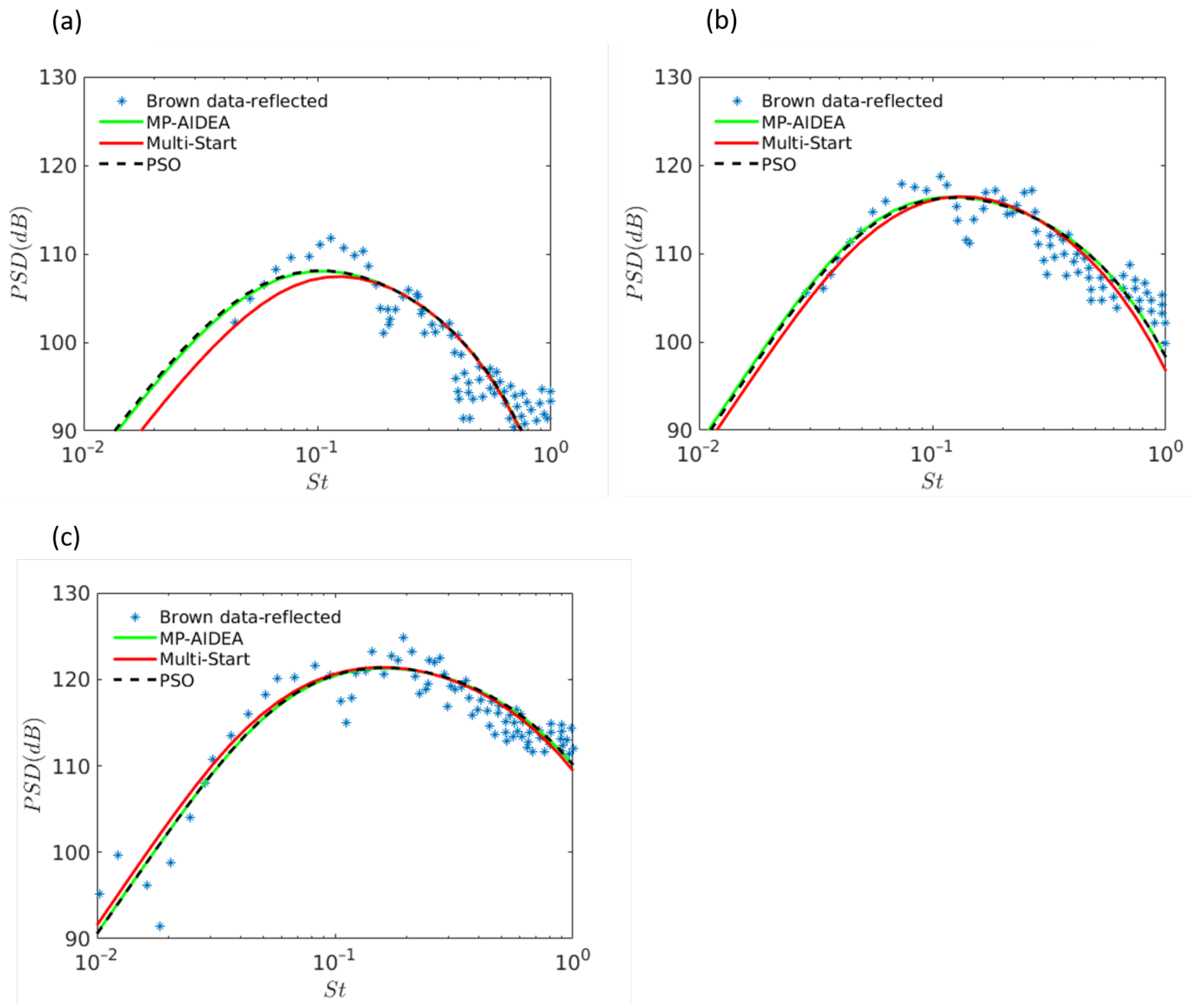
Method 1 was used to find the four parameters through optimization of our acoustic model against the experimental data in [12]. Figure 10 shows that the predictions are particularly good for $Ma=0.7$, and $Ma=0.9$ for all optimization routines. For $Ma=0.5$ Multi-Start gives a poorer prediction due to the change in $l_3$ which affects low frequency roll-off. From this figure, it is shown that MP-AIDEA and PSO give more or less the same acoustic predictions for all acoustic Mach numbers.

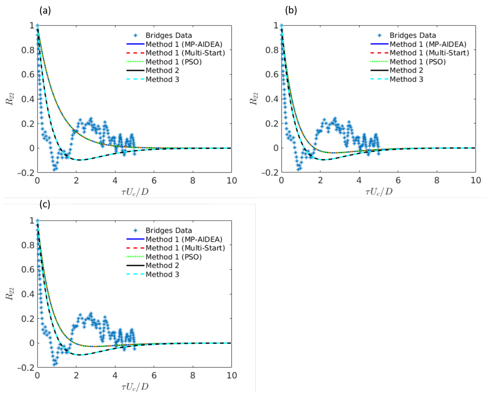
However, the turbulence correlation function $R_{22}$ that we use (Equation (5)) is a function of $a_1$, and the values for $a_1$ that were found from this method for each optimization routine do not give a good representation of $R_{22}$, as shown in Figure 9. The initial decay is too slow and there is little to no anti-correlation region, this is particularly the case for $Ma=0.5$. Note, that we’ve allowed $\tau U_c/D\to 10$ to show where the model goes to zero, there is no turbulence data at these locations most likely due to measurement difficulties.

In methods 2 and 3, we optimized the $R_{22}$ model separately against experimental data from Bridges ($y_1/D=6,r/D=0.5$) [36]. This means that the anti-correlation region is represented and the initial decay is steeper, as shown in Figure 9 for methods 2 and 3. Only the initial de-correlation is of interest, therefore we have used a simple model for $R_{22}$. A different model could be used to capture the oscillations but this would make the acoustic model much more complicated and have no improvement on the acoustic spectrum predictions.

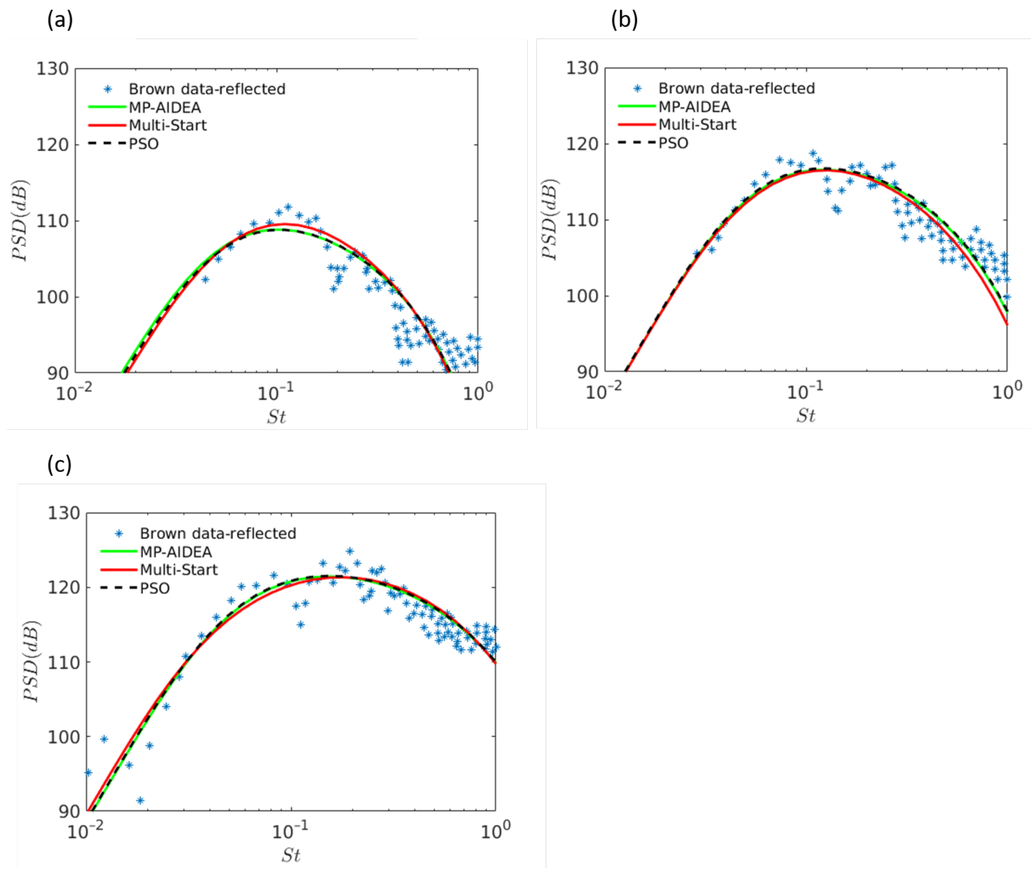
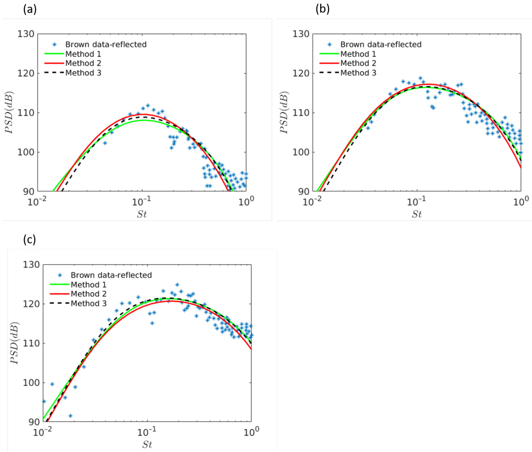
For method 3 we use the this $R_{22}$ optimized value $a_1$ ($0.85$) in the acoustic model and then optimize the other parameters against the acoustic data to find the best prediction. This allows us to find the optimal predictions for the acoustic spectrum while also having a good representation of the turbulence structure. It results in slightly poorer acoustic predictions, with the exception of Multi-Start for $Ma=0.7$, as noted in Table 2, Table 3 and Table 4. However, Figure 11 shows that they still give very good predictions for the level of accuracy that we require. Since this method also allows $R_{22}$ to be better represented, overall it is deemed to be better than method 1.

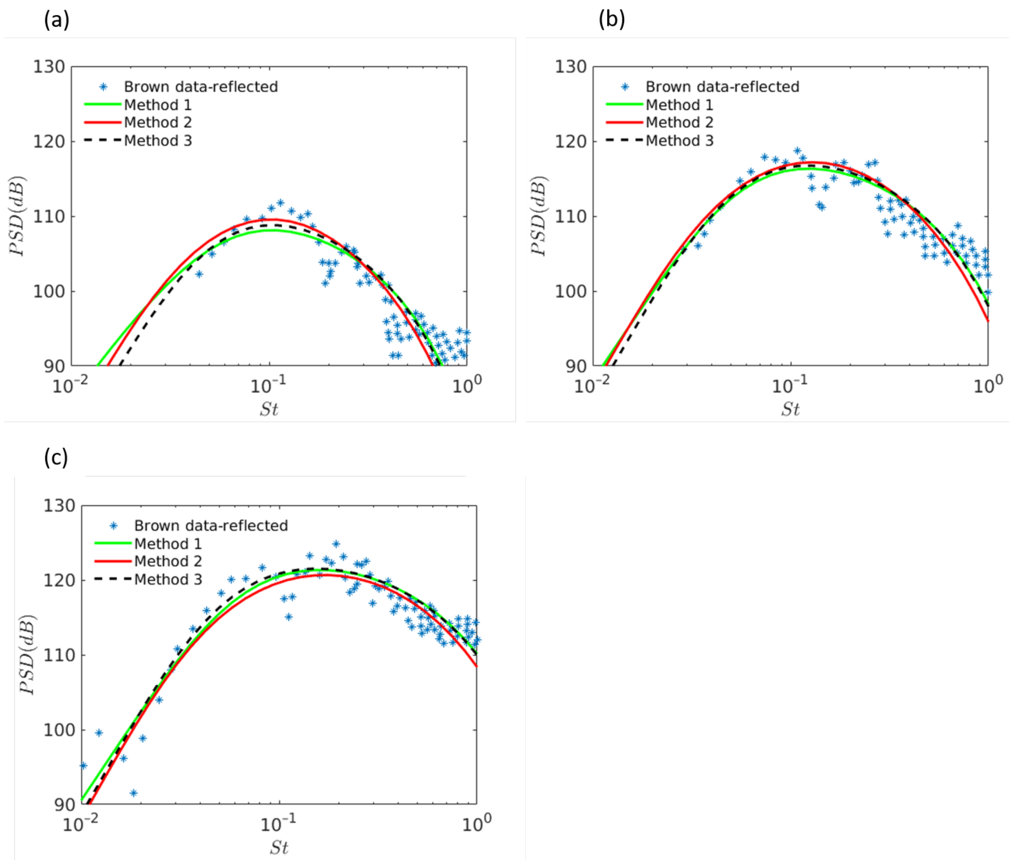
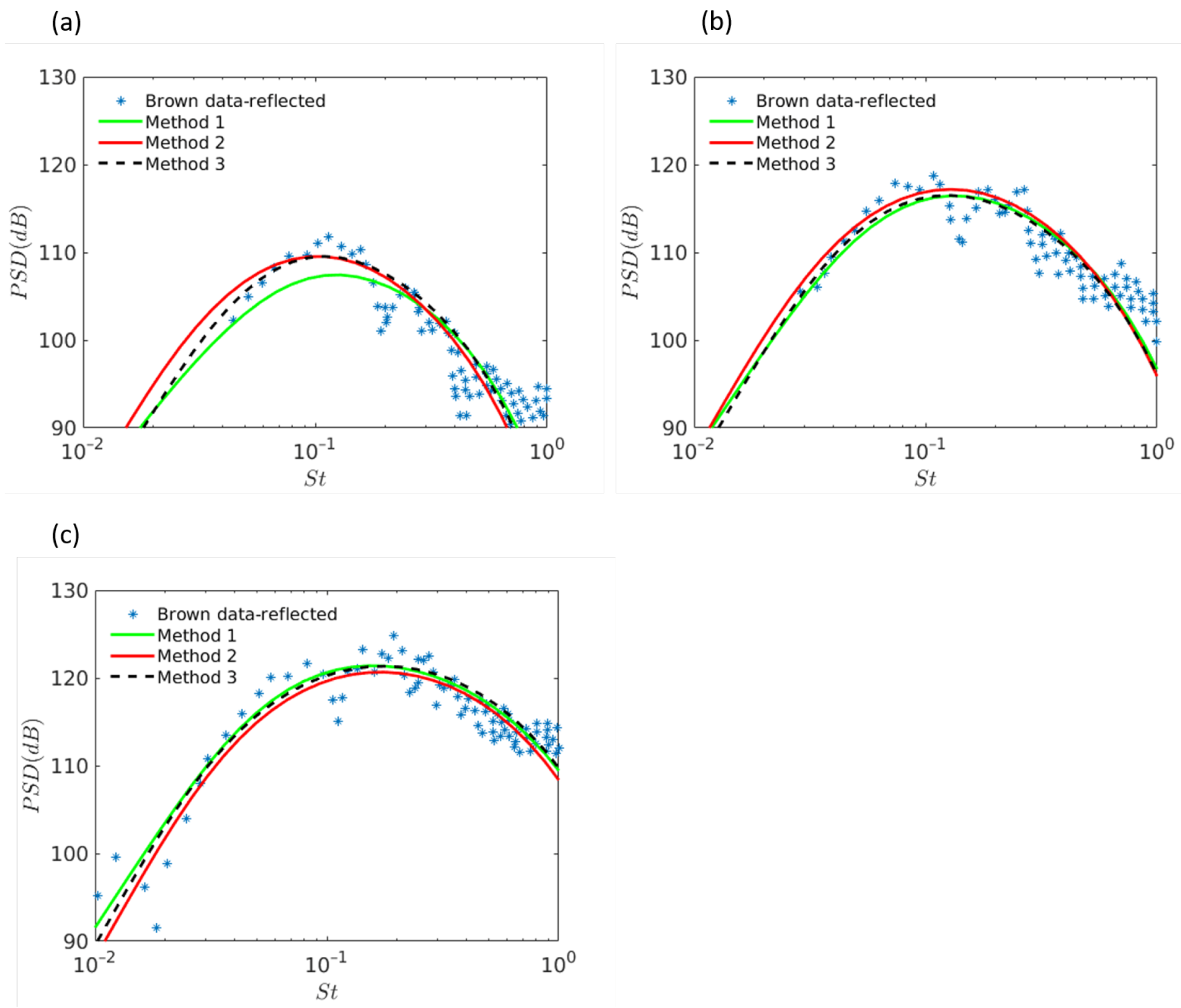
In method 2, we also use this value ($a_1=0.85$) in the acoustic model and hand tune the other parameters to find the best prediction. We aimed to find one set of parameters for all acoustic Mach numbers. However, it was found that due to the level shift in the acoustic spectrum, one parameter ($l_2$) must change for each Mach number. As this method did not require different optimization routines, the results are included in Figure 12, Figure 13 and Figure 14 and is identical in each. We can see that the predictions are similar to methods 1 and 3. However, hand tuning these parameters is not ideal as it relies on human judgement as to what is a ‘good’ prediction.

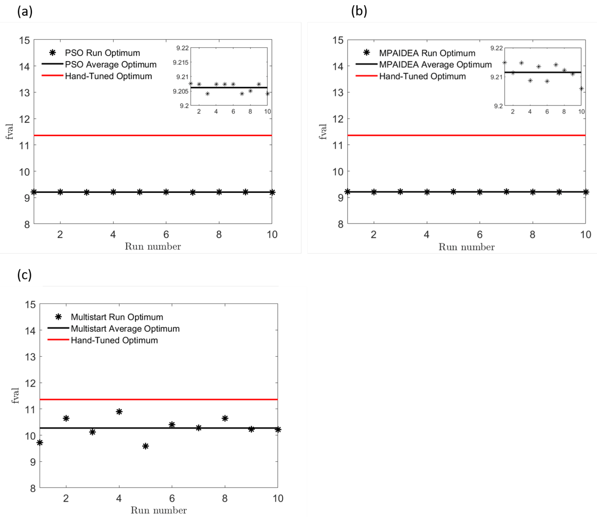
It is easy to see in Figure 12, Figure 13 and Figure 14 that the three methods of optimization give similar acoustic predictions for all optimization routines, with only Multi-Start giving a noticeable change in prediction for $Ma=0.5$. Note that from Figure 8 only PSO and MP-AIDEA consistently converged to a minimum objective function value ($fval=9.2$), Multi-Start displayed a more widely varying value, possibly due to the number of starting points chosen (500). 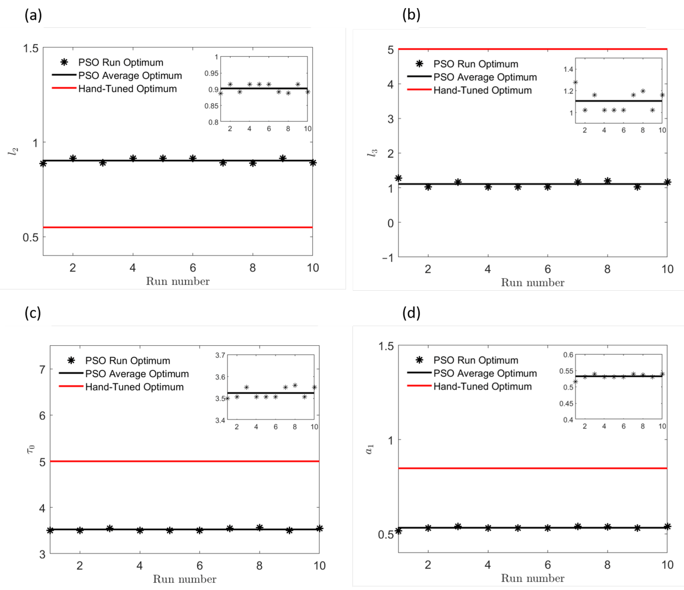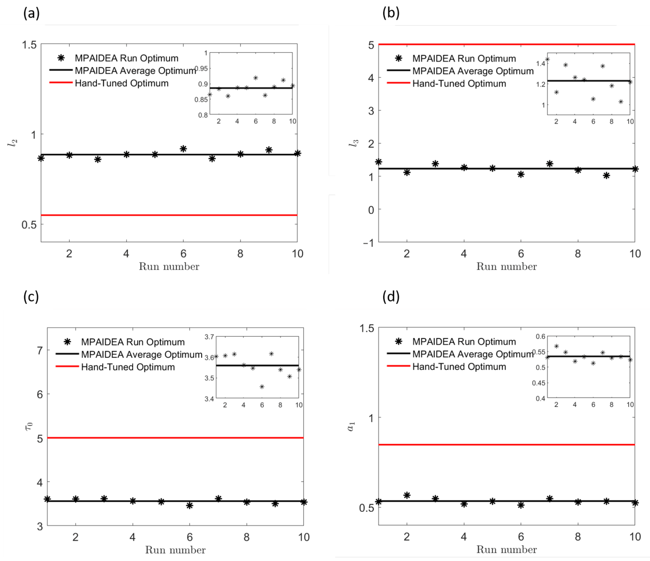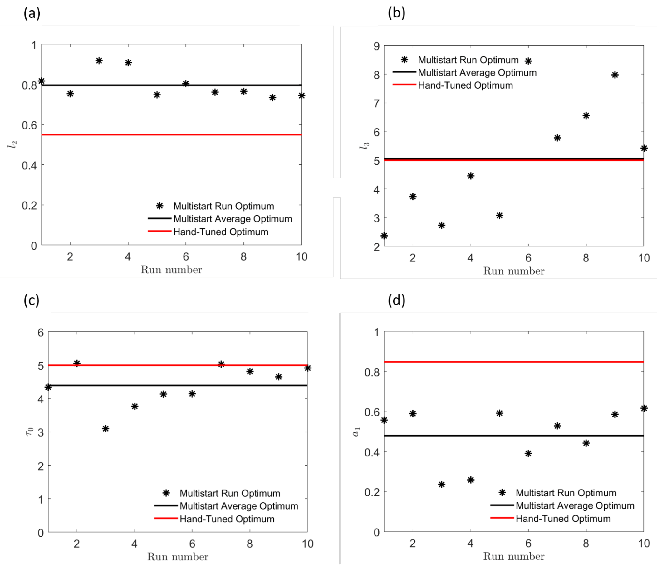Figure 7 shows that the parameters found for Multi-Start also vary widely on each run of the routine, hence it is less likely that acoustic predictions found using Multi-Start are optimal. On the other hand, Figure 5 and Figure 6 show that the parameters found by PSO and MP-AIDEA respectively, only vary slightly.

We can conclude that our acoustic spectrum model for the trailing-edge noise problem is ‘parametrically flat’, i.e., the objective function is not noticeably sensitive to the variation of parameters $(l_2,l_3,a_1,{\tau }_0)$ within their specified range. Both evolutionary optimization routines that we have used in this paper have given good results and almost identical predictions. The time taken in optimising method 1 naturally took longer than method 3 since an extra parameter was being found. In general, it was found that method 1 was faster using PSO, however method 3 was faster using MP-AIDEA. However, for the number of starting points that was chosen, Multi-Start was fastest of all, and since the objective function value was still smaller than method 2, if there was a time constraint which restricted the use of evolutionary algorithms, it would be worthwhile to use Multi-Start rather than hand-tuning the problem.

7. Conclusions

Aeroacoustic models for turbulence interaction problems will always require a set of parameters that define the rate of temporal and spatial de-correlation. For the trailing-edge noise problem as illustrated in Figure 1, the acoustic spectrum (Equation (2)) is proportional to the Fourier transform of the streamwise-independent transverse velocity correlation function, $R_{22}(\tilde{u}-u,\tilde{v}-v;\omega )$ via Equations (3), (4) and (6) and depends on $\mathcal{O}\left(1\right)$ parameters $(l_2,l_3,a_1,{\tau }_0)$. The latter can be chosen by hand-tuning, however this will not result in a ‘mathematically’ optimal choice of parameters, and could result in under/over prediction of the acoustic spectrum (as illustrated in Figure 12, Figure 13 and Figure 14). It also adds to the time taken in assessing its predictive capability. This paper highlights how optimization routines, both evolutionary and non-evolutionary, can be used to determine what the optimal parameters are, resulting in slightly better acoustic predictions (see Figure 12, Figure 13 and Figure 14). When determining turbulence-associated parameters in acoustic models for which more than the 3 state variables considered in this paper (i.e., $Ma,\theta ,\varphi$) are required, such as in predictive models of the full jet-installation noise signature, the use of a numerical optimization routine will become even more beneficial.