Evaluation of Human Resources in Transportation Companies Using Multi-Criteria Model for Ranking Alternatives by Defining Relations between Ideal and Anti-Ideal Alternative (RADERIA)

Abstract

Multi-criteria decision-making methods (MCDM) represent a very powerful tool for making decisions in different areas. Making a rational and reliable decision, while respecting different factors, is a challenging and difficult task; MCDM models have a great impact on achieving this goal. In this paper, a new MCDM technique is presented—ranking alternatives by defining relations between the ideal and anti-ideal alternative (RADERIA), which was tested for the evaluation of human resources (HR) in a transportation company. The RADERIA model has three key advantages that recommend it for future use: (1) the RADERIA model has a new approach for data normalization that enables defining the normalization interval according to the judgments of a decision-maker; (2) an adaptive model for data normalization of the RADERIA model allows tough conversion into various forms of decreasing functions (linear, quadratic equation, etc.); and (3) the resistance of the RADERIA model to the rank reversal problem. Furthermore, in many simulations, the RADERIA method has shown stability when processing a larger number of datasets. This was also confirmed by a case study with 36 alternatives, as considered in this paper. The results and verification of the proposed new method were acquired through a comprehensive verification of the complexity of the results. The complexity of the results was executed through (1) comparison with four other multi-criteria methods, (2) checking the resistance of the RADERIA model to the rank reversal problem, and (3) the analysis of the impact of changes in the measurement scale on the ranking results.

1. Introduction

Managing a successful business in any field depends primarily on the ability to maintain the needs and meet the expectations of all participants in the examined chain. It is necessary to define the goals and strive to achieve them. Logistics plays an important role in this, giving the answers to the question of how to rationalize, considering primarily the performances that have the most impact on rationalization. Lately, especially in the past few years, even companies in developing countries have recognized the importance of logistics in the rationalization of their entire system. According to [1], rationalization of logistics activities and processes is very important in doing business and achieving efficiency in a company. This is also confirmed by Koskinen and Hilmola [2]; according to them, the rationalization of the basic logistics subsystems is the key factor in achieving efficiency and effectiveness in companies. On the one hand, in the structure of the basic logistics subsystems, transportation presents the subsystem with the largest structure of logistics costs expressed on a daily basis, especially in large transportation companies. This is confirmed by Guasch [3] who emphasizes that the transportation costs represent the most important part of all logistics costs—percentage participation determined by Rantasila and Ojala [4]. They calculated that more than a third, or more precisely around 40%, of all logistics costs are made by transportation subsystems. On the other hand, this logistics subsystem enables achieving the purpose and goals of logistics, thanks to its importance and irreplaceability. Borzacchiello et al. [5] also confirm this, emphasizing that in today’s modern economic system, transportation represents dynamic part, especially because it achieves great economic benefits and increases economic growth. In such companies, the rationalization of their activities plays a significant role in providing business efficiency [6]. Taking all of the above into consideration, it is necessary to constantly monitor the indicators that are responsible for making transportation costs, then focus on these performances and strive to improve them because they have an enormous impact on increasing the efficiency of transportation activities, as well as reducing time and costs.

To rationalize costs acquired through different transportation activities and processes, it is necessary to obtain adequate management and define adequate strategies [7]. According to Stević et al. [1], this can be seen especially in big and medium transportation companies, which is the case in this research. As already stated, in recent years, companies have realized the significance of logistics and they have started managing logistics, i.e., transportation costs. Furthermore, it is necessary to pay attention to the rolling stock, its structure, drivers, and management; according to Stojić et al. [8], the rolling stock represents the essential importance of the effective functioning of transportation companies. Higher rate mobility, which has become our everyday reality, causes a higher frequency of commodity flows, which contributes to the increasing importance of freight transport, and, according to Ghiani et al. [9], it plays a key role in today’s economies.

Taking into consideration all of the above-mentioned, it is necessary to create great management and carry out adequate managing decisions in transportation companies. Basically, transportation companies that are working as logistics providers have to provide the required quality service for a minimal price. The outsourcing approach is, according to Liu et al. [10], widely present in all logistics aspects of business, especially in the field of transportation, characterized by significant and direct participation in total logistics costs. Transportation companies that are working as logistics outsourcing are largely dependent on the quality of the rolling stock, i.e., transportation vehicles [11], and therefore on HR, too, that is, the drivers.

If we observe the entire transportation market with a large number of transportation (logistics) companies, reducing the company’s costs is a mandatory factor in order to achieve greater competitiveness. In transportation service companies, the largest share of costs is fuel consumption that is, consciously or unconsciously, influenced by the drivers themselves. One of the ways to decrease fuel consumption is the implementation of eco training for the drivers [12], or implementation of a reward system for drivers who achieve higher performance, i.e., the lowest fuel consumption. As a result of the training, reduction in fuel consumption can be higher than 10%; for example, in the study [13], 13.6% on average was achieved. In addition, the integration of these two approaches could have an adequate impact on reaching the target function. We should take into account the fact that, according to the performed study in [14], truck drivers were found to be happier during off-job activities. Therefore, managers of transportation companies should constantly work on increasing the satisfaction of their drivers. According to study [15], the high demands of their jobs can lead them to overlook their health, which can negatively impact every participant in supply chains.

In this paper, research was carried out in a company that is primarily engaged in international transportation and works on the EU territory. It was found that there are large differences in fuel consumption depending on the driver, even when it comes to the same transport routes. Therefore, an evaluation of the drivers was conducted in this paper, taking five criteria into consideration, where gas consumption is the most significant. A multi-criteria decision-making model (MCDM) was formed, and for these purposes, a new MCDM method called RADERIA was developed, which defines relations between an ideal and anti-ideal alternative and in that way, it respects their correlations, which can have a high impact on forming the final model, or on reaching a final decision. Solving the problem this way represents a new direction in the field of multi-criteria decision-making, which can have a positive impact on the entire field.

Based on everything outlined in this study, several important goals can be identified. The first goal is to form an adequate model for managing HR in transportation companies in order to achieve effectiveness and efficiency. This includes evaluating the work of the drivers on a monthly basis using five criteria, as well as additional money rewards for the best ranking drivers. The second goal represents the development of the new RADERIA method in order to get the MCDM method that also respects different variability factors and eliminates the rank reversal problem, which is present in many MCDM models. The third goal of this paper represents the contribution of Prospective Multiple Attribute Decision Making (PMADM) as defined in [16].

The present paper contains seven sections. The first section introduces the motivation of the research, objectives, and importance of the field. The second section shows the literature review in which similar problems in managing HR in transportation and logistics companies are analyzed. After that, in the third section, the methodology developed in this paper is presented. It implies defining all the steps for carrying out the research, implementing the LBWA method for determining the importance of data as well as the new RADERIA method. The fourth section consists of the study case where the advantages of the developed methodology are represented. In the fifth section, the validity analysis is conducted by comparing the developed methodology and other methodologies using different scenarios. The sixth section consists of a discussion on the obtained results and reviewing the advantages of the new method. Contributions and future research are described in the seventh section.

2. Literature Review

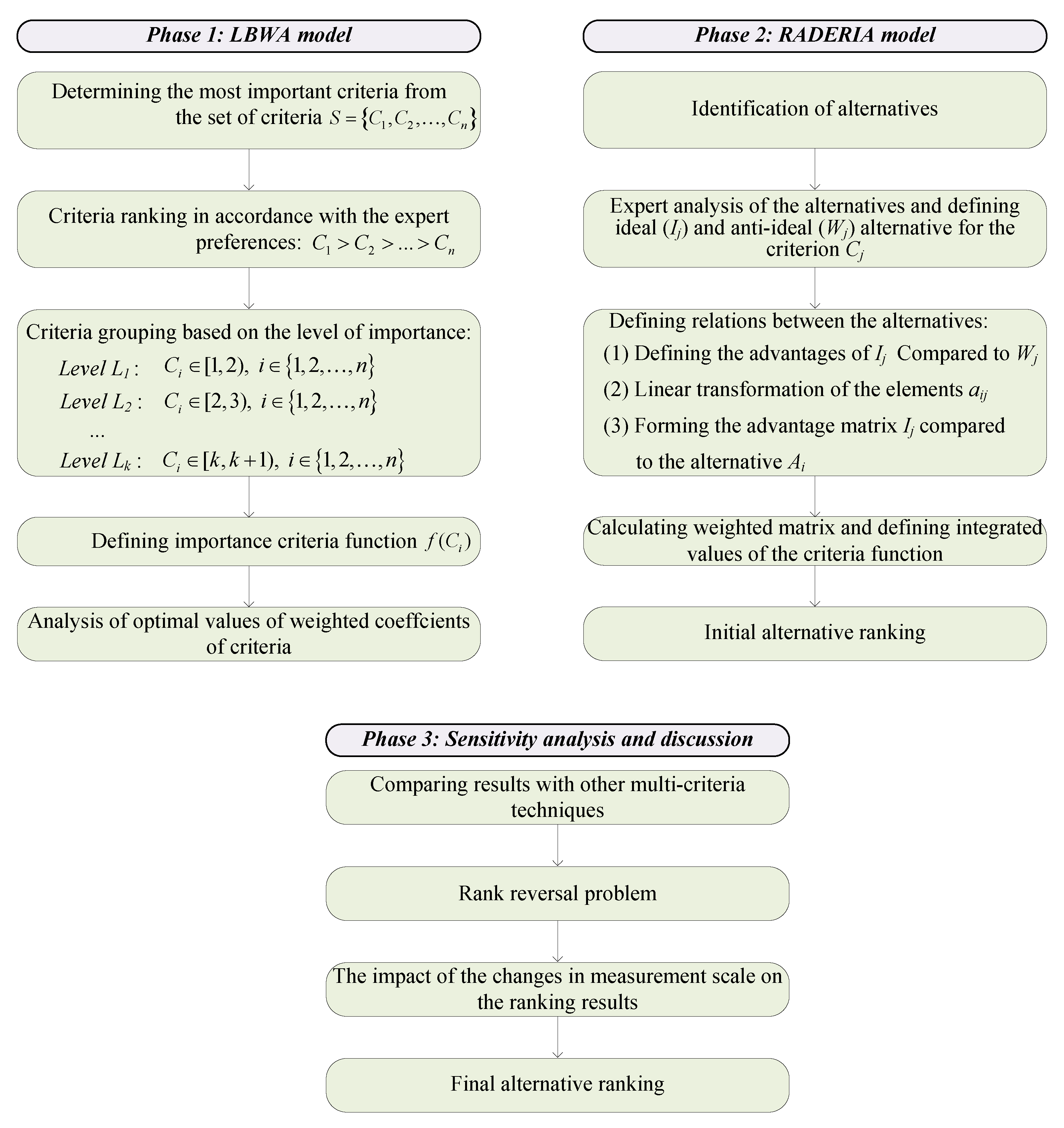
Micro, small and medium companies are popular and suitable for considering the implementation of the concept of business process management [17]. Based on the above, it is possible to see a necessity for creating a model for evaluating human performance [18], especially because, according to Gürbüz and Albayrak [19], human performance assessment is one of the key areas for analysis of the continuity of a company. This was confirmed in a study [20] where the authors noticed that companies can form and keep a competitive advantage by leveraging the expertise of HR development. One of the benefits of this study is the creation of a model for evaluating the work performance of drivers periodically based on multiple parameters, which has not been observed in the literature so far. Transportation, as a part of a supply chain, often represents an area of interest for various authors from different aspects, but not from the mentioned aspect.

According to Dubey and Gunasekaran, [21] can be a remark that drivers do not care about the environment or society, as manifested in their behavior. Therefore, they should have skills that make them more ecologically aware. Essentially, the goal of studying such problems and optimizing them leads to the achievement of environmental, economic, and social optimization aspects. Adequate choice and evaluation of staff in logistics represents an extremely significant factor of optimization because Klumpp and Abidi [22] noticed that one of the most significant tasks in logistics in the future is the evaluation and choice of workers in accordance with their competences and knowledge levels. Wu and Hou [23] carried out research on evaluating workers in a distributive center in Taiwan. The goal of their study was the development of employee performance estimation (EPE), which included three different models: direct performance determination (DPD), indirect performance determination (IPD), and performance score analysis (PSA). Workers on different levels were evaluated: 36 distinct first-line operators, 4 office-level managers, and 2 division-level managers. Chang [24] evaluated six employees in logistics companies according to four criteria: potential for future, corporate business achievement, organizational commitment, and working ability. He applied an integrated MCDM model, which consists of the Analytic Hierarchy Process (AHP) and technique for order preference by similarity to an ideal solution (TOPSIS). Paper [25] shows the modeling and evaluating of five different strategies in HR areas in an Indian logistics company using system dynamics modeling. This study also explored the impact of employees on the logistics performance index. After the study was carried out, the results were presented as a percentage for each investing strategy. Kampf and Ližbetinová [26] in their study used the AHP method in order to identify talents in logistics as one way to improve market competitiveness. Their goal was, after identifying such HR, to bring new values so that the company could optimize their business. Similar research was done by Qu et al. [27] and Badi et al. [28] who used the AHP method and triangle-definite weighted functions. The received results can be used as a reference for the companies in making the right and best decision on talents and provide long-term development strategies.

Xin et al. [29] state that talent is the most precious resource in the modern world, which was also confirmed in a study by Li et al. [30]. They carried out research whose aim was the application of fuzzy comprehensive appraisal in the human capital evaluation of logistics companies.

The purpose of carrying out such evaluations, according to Yue [31], is to understand the compatibility level between the demands of the workplace and the employees. In this research, according to the same author who applied the AHP method, it was given the possibility of acquiring a clearer perspective of the condition in the HR area in a logistics company by applying adequate measures and strategies. Samad [32] carried out research in the logistics sector on 292 employees. This study presents the findings of a study that examined the relationship between organizational justice and employees’ work outcomes. In [33], research was performed in the area of logistics distribution and it was explained that HR, and investing in these intangible assets, can contribute to improving company performance and increasing competitiveness in the market. In a research conducted by Gürbüz and Albayrak [19], a model for evaluating employees in a pharmaceutical company marketing sector was presented. Analytical Network Process (ANP) and Choquet Integral (CI) were applied simultaneously to perform an adequate evaluation.

3. Methodology

In this part of the paper, a methodology for evaluating drivers in a logistics organization is presented. The methodology for evaluating drivers consists of three phases, as shown in Figure 1.

In the first phase, an expert team group has to be formed, and the set of alternatives is formed, as are criteria for evaluating alternatives. In the second phase, weighted coefficients are calculated using the LBWA (Level Based Weight Assessment) method. Weighted coefficients obtained in this phase are used further on in the RADERIA model for evaluating drivers. A detailed review of the steps in the LBWA–RADERIA multi-criteria model is shown in the following part.

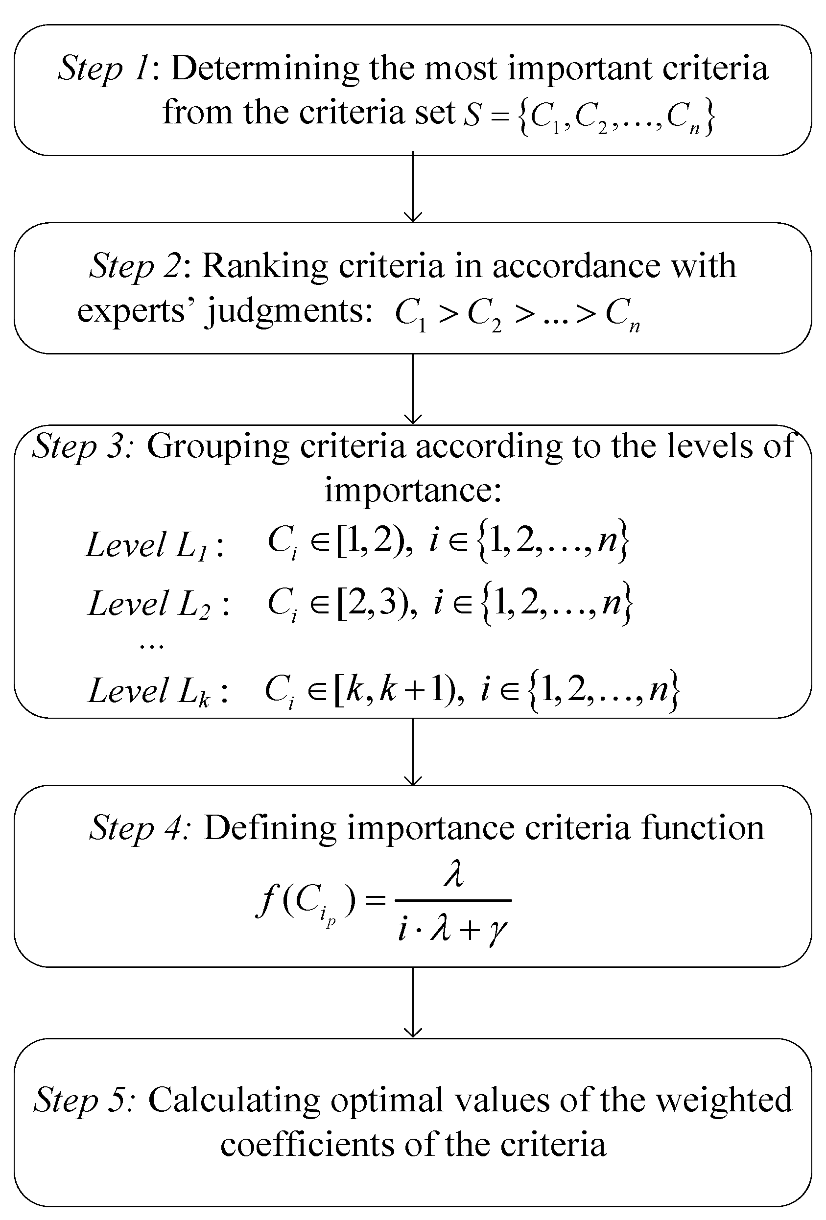
3.1. The LBWA Model for Determining Weighted Coefficient of the Criteria

The LBWA model is based on a pairwise comparison of the criteria through forming a non-decreasing array of the criteria importance levels. Methods that subjectively determine the weighted coefficients of the criteria focus on the information obtained based on the judgments of the decision-makers [34]. This model implies the use of an original algorithm for grouping criteria based on the level of importance in order to eliminate the need for predefining an ordinary scale for pairwise comparison of the criteria. After grouping levels, the judgments of the decision-makers are defined [35] because modeling expert judgments in decision-making problems [36] is an interesting field of research. This way, it is possible to obtain relations between criteria that satisfy the condition of maximal consistency and also represent realistic relations, which are defined through expert judgments. The proposed model eliminates inconsistencies in expert judgments which can be seen in other famous models (Best–Worst Method—BWM and AHP) because the LBWA results are always highly consistent. We emphasize this because when increasing the level of consistency in the AHP and the BWM, expert judgments are distorted as a result of the violation of the consistency of the model. The mentioned problem is often due to the use of the nine-point scale, which has limited possibilities for expressing expert judgments [37]. The LBWA model has the following advantages: (1) enables rationally expressing the judgments of a decision-maker with a minimal number of comparisons, n − 1; (2) eliminates the shortcomings of nine-point that are described in many studies (Asadabadi et al., 2019); and (3) the shown model has great flexibility while expressing expert judgments and it eliminates discrepancies which can occur with models that use the pairwise comparison technique. The LBWA algorithm is shown in Figure 2.

Detailed explanation of the steps that are used in the LBWA algorithm can be seen in the paper written by Zizovic and Pamucar [35].

3.2. Ranking Alternatives by Defining the Relationship between Ideal and Anti-Ideal Alternatives (RADERIA)

A multi-criteria model with n criteria $C_1,C_2,\dots ,C_n$ is given. Criteria are aligned according to their importance $C_1>C_2>C_3>\dots >C_n$ based on subjective judgments of a decision maker, while two or more criteria can be of the same importance. We shall assume that there is m alternative which is denoted by $A_1,A_2,\dots ,A_m$. To each of these alternatives $A_i$ ($i=1,2,\dots ,m$) on the criterion $C_j$ ($j=1,2,..,n$), $a_{ij}$ value is added and the initial decision-making matrix $X={\left[a_{ij}\right]}_{m\times n}$ is formed. The criteria can be of the maximization or minimization type. We shall assume that all criteria are of the maximization type (which does not minimize the generality). Based on the defined settings of the multi-criteria model, the following steps of the RADERIA model are presented.

Step 1. For each criterion $C_j$ ($j=1,2,\dots ,n$), a decision-maker determines the ideal value for the alternative $I_j$ and anti-ideal value for the $W_j$, where the following condition exists $W_j<I_j$ ($j=1,2,\dots ,n$). Anti-ideal value ($W_j$) represents the least acceptable value for the decision-maker on the given criterion, while the ideal value represents the most acceptable value on the given criterion. The values $I_j$ and $W_j$ can be defined using the set of the alternatives $A_i$ on the criterion $C_j$, but mainly they are given the values which are not in the set of the considered alternatives.

Step 2. Defining the advantage of $I_j$ compared to $W_j$; A decision-maker defines how many times the ideal alternative $I_j$ is better than the anti-ideal alternative $W_j$ with respect to the criterion $C_j$ ($j=1,2,\dots ,n$). Here, we should emphasize that the term “better alternative” is not the same as “bigger alternative”. We stress this because these two terms are constantly used as synonyms. For example, if we observe two alternatives (A₁ and A₂) with respect to the criterion C₁, $A_1=5$ and $A_2=15$ (assume that the values are defined based on a ratio scale), we can say that the alternative $A_2$ is bigger than the alternative $A_1$ by three times, exactly. At the same time, we can estimate that the alternative $A_2$ is better than the alternative $A_1$ by five times.

Let us have ${\alpha }_j$ (${\alpha }_j>1$) that is a value which determines how many times $I_j$ is better than $W_j$. The limit values ${\alpha }_j^{(I_j)}$ and ${\alpha }_j^{(W_j)}$ for every criterion $C_j$ are defined in the same interval. Simultaneously, the decision-maker defines $k_j$ points $(k_j\ge 1)$ from the interval $\left[W_j,I_j\right],$ $e_{1,j},e_{2,j},\dots ,e_{k_j,j}$ where $e_{k_j+1,j}=W_j<e_{k_j,j}<e_{k_j-1,j}<\dots <e_{2,j}<e_{1,j}<I_j=e_{0,j}$, that satisfies the following:

• $I_j$ is ${\alpha }_j^{(1)}$ times better than $e_{1,j}$
• $I_j$ is ${\alpha }_j^{(2)}$ times better than $e_{2,j}$
• ...
• $I_j$ is ${\alpha }_j^{(k_j)}$ times better than $e_{k_j,j}$

The values ${\alpha }_j^{(i)}$ are aligned according to their importance ${\alpha }_j^{(k_j+1)}$ > ${\alpha }_j^{(k_j)}$ > ${\alpha }_j^{(k_j-1)}$ >...> ${\alpha }_j^{(2)}$ > ${\alpha }_j^{(1)}$. That is how $k_j+1$ interval is defined. For example, if alternative $A_i$ has value $a_{ij}$ in interval $e_{s+1,j}<a_{ij}\le e_{s,j}$, then $I_j$ is better than the alternative $A_i$ by exactly ${\alpha }_j^{(s)}$ times. At the same time, the alternative $A_i$ is ${\alpha }_j^{(s+1)}$ times smaller than $I_j$.

Step 3. Forming the advantage matrix $I_j$ compared to the alternative $A_i$, $\overline{X}={\left[{\alpha }_{ij}\right]}_{m\times n}$: In this step, we define how many times the ideal alternative ($I_j$) is better than the alternative $A_i$. Let us have the value for the alternative $A_i$ with respect to the criterion $C_j$ defined in the initial decision-making matrix $X={\left[a_{ij}\right]}_{m\times n}$. Then, if the value is $a_{ij}$ where $e_{s+1,j}<a_{ij}\le e_{s,j}$ ($s=0,1,\dots ,k_j$), then it will be as follows:

If $a_{ij}=e_{s,j}$, then the alternative $I_j$ is better than $A_i$ by exactly ${\alpha }_j^{(s)}$ times.

If $a_{ij}<e_{s,j}$, then the alternative $I_j$ is ${\alpha }_j^{(i)}$ times better than $A_i$, where ${\alpha }_j^{(i)}$ is defined using Expression (1):

$${\alpha }_j^{(i)}={\alpha }_j^{(s)}+\frac{({\alpha }_j^{(s+1)}-{\alpha }_j^{(s)})(a_{ij}-e_{s,j})}{e_{s+1,j}-e_s}$$

(1)

If $a_{ij}=W_j$, then ${\alpha }_j^{(i)}={\alpha }_j$, or $I_j$ is better than $A_i$ exactly ${\alpha }_j$ times. This happens only when the alternative $A_i$ uses $a_{ij}$ for its limiting value from the intervals $\left[W_j,e_{k_j,j}\right]$.

The relation between $I_j$ and the alternatives $A_i$ and $W_j$ is shown in Figure 3.

In Figure 3, we can see that the value ${\alpha }_j^{(i)}$ can be defined using decreasing functions. In Figure 3a, the values ${\alpha }_j^{(i)}$ are shown using a linear function, which is represented with Expression (1). However, values ${\alpha }_j^{(i)}$ can be defined with other decreasing functions, such as with the quadratic function, etc. (Figure 3b).

After defining values ${\alpha }_j^{(i)}$ for each alternative $A_i$ with respect to the criterion $C_j$($j=1,2,\dots ,n$), we get the advantage matrix of the alternative $I_j$ compared to the alternative $A_i$ ($i=1,2,\dots ,m$) (Expression (2)).

$$\overline{X}=\left[\begin{array}{cccc}{\alpha }_{11}& {\alpha }_{12}& \cdots & {\alpha }_{1n}\\ {\alpha }_{21}& {\alpha }_{22}& \cdots & {\alpha }_{2n}\\ ⋮& ⋮& \ddots & ⋮\\ {\alpha }_{m1}& {\alpha }_{m2}& \cdots & {\alpha }_{mn}\end{array}\right]$$

(2)

Step 4. Defining weighting matrix $\overline{U}={\left[u_{ij}\right]}_{m\times n}$. Let us have weighted coefficients for all criteria, where ${\displaystyle \sum _{j=1}^n{w}_j}=1$, $w_j>0$ ($j=1,2,\dots ,n$) and satisfy the condition $w_1\ge w_2\ge ,\dots ,\ge w_n$. Multiplying elements of the matrix $\overline{X}={\left[{\alpha }_{ij}\right]}_{m\times n}$ with the weighted coefficients of the criteria $w_j$, we get the weighted advantage matrix of the ideal alternative compared to the alternative $A_i$:

$$\overline{U}=\left[\begin{array}{cccc}{u}_{11}& u_{12}& \cdots & u_{1n}\\ u_{21}& u_{22}& \cdots & u_{2n}\\ ⋮& ⋮& \ddots & ⋮\\ u_{m1}& u_{m2}& \cdots & u_{mn}\end{array}\right]$$

(3)

For values $u_{ij}$ we get $u_{ij}={\alpha }_{ij}\cdot w_j$, ($i=1,2,\dots ,m$; $j=1,2,\dots ,n$).

Step 5. Determining the final value of the criteria function: Adding elements of the matrix $\overline{U}={\left[u_{ij}\right]}_{m\times n}$ by columns, we acquire final values of the criteria alternative functions (Expression (4)):

$$Q{(A_i)}_k={\displaystyle \sum _{k=1}^n{u}_{ik}}$$

(4)

It is obvious that, if for all values $A_i$ $\in$ ($I_1$, $I_2$,..., $I_n$) for each $j$ ($j=1,2,\dots ,n$), then ${\alpha }_j=1$, so

$$Q(A_i)=w_1+w_2+\dots +w_n=1$$

(5)

In the case that $A_i$ for all values $a_{ij}$ has anti-ideal values, that is $A_i$ $\in$ ($W_1$, $W_2$,..., $W_n$), then:

$$Q(A_i)={\alpha }_1^{(i)}{w}_1+{\alpha }_2^{(i)}{w}_2+\dots +{\alpha }_n^{(i)}{w}_n={\displaystyle \sum _{k=1}^n{u}_{ik}}$$

(6)

Then we can state that $Q(A_i)$ satisfy the condition where $1\le Q(A_i)\le {\displaystyle \sum _{k=1}^n{u}_{ik}}$.Values $Q(A_i)$ show how many times the alternative $A_i$ is weaker than the ideal alternative.

Step 6. Ranking alternatives: Ranking alternatives is done based on the values of the criteria function—$Q(A_i)$. In order for the alternative to be as highly ranked as possible, it is preferable to have the lowest value $Q(A_i)$:

(1) Let us have $A_x$ and $A_y$, two arbitrary alternatives, and let us have the following values $Q(A_x)$ and $Q(A_y)$; then, if $Q(A_x)$ > $Q(A_y)$, it is true that $A_x$ → $A_y$. Sign “→” represents domination of the alternative $A_x$ compared to the alternative $A_y$.

(2) If the condition $Q(A_x)$ = $Q(A_y)$ is satisfied, then it will be as follows:

• From the matrix $\overline{U}={\left[u_{ij}\right]}_{m\times n}$ we eliminate the values of all alternatives based on the weakest criteria, and from such a reduced matrix we can observe the new values $Q(A_x)$ and $Q(A_y)$. If the condition $Q(A_x)$ > $Q(A_y)$ is satisfied, then $A_x$ → $A_y$.
• If it is still $Q(A_x)$ = $Q(A_y)$ even after eliminating the weakest criterion, then the next weakest criterion is eliminated. We repeat this until we get $Q(A_x)$ ≠ $Q(A_y)$. Then, if we, for example, get $Q(A_x)$ < $Q(A_y)$, then $A_y$ → $A_x$.
• If the equality $Q(A_x)$ = $Q(A_y)$ still exists even after eliminating all the criteria, then we analyze if any of the alternatives, $A_x$ and $A_y$, on the criterion $C_j$ acquire values which are better than the value which was defined as the ideal alternative on the criterion $C_j$. In the case that there is such an alternative, then that alternative is chosen as the better one.
• If the equality $Q(A_x)$ = $Q(A_y)$ still exists even after eliminating all the criteria, then we can say that the alternatives $A_x$ and $A_y$ are equal.

4. Case Study and Experimental Results

The research was carried out in a transportation company for international transportation. For each subsystem in the company, elements for improvement were determined. In order to create an action plan for improving the performance of the company, it was concluded that HR represents the critical factor for the business that can be significantly improved. Even though there exists an adequate motivational system for the employees, i.e., truck drivers, HR represents the focus for improvement because the adequacy of the transportation depends mainly on them. It was concluded that there is a need for a periodical evaluation of the drivers, rewarding two to three of the best drivers, and also a need for creating such a multi-criteria model.

In order to find an adequate solution, a model for evaluating drivers is formed based on five quantitative and qualitative criteria. The first criterion (C1) represents fuel consumption expressed in liters per 100 km. This criterion is quantitative and of the costs type. The company manages very meticulous paperwork on every kilometer driven and fuel consumption, so this data was taken from the database. The second criterion (C2) is also quantitative and of the costs type, and it refers to the damage per km, expressed in money value damage on the vehicle, caused by driver’s carelessness. This criterion includes all damages, from the small ones to the large ones, which are very rare. The other three criteria are of a qualitative character and of the useful type. The third criterion (C3) implies the adequate maintenance of the vehicle by the drivers, periodically examined by the managers of the company.

The fourth criterion (C4) represents the driver’s ability to give adequate information on time. This mainly refers to the driver’s ability to manage adequate communication with the dispatchers, especially in unexpected situations, which are very common in the transportation process. The fifth criterion (C5) represents loyalty that can be seen through the execution of all duties without complaint and also the driver’s flexibility in executing their tasks.

4.1. Determining Criteria Weights Using the LBWA Model

For determining criteria weight, the LBWA model [35] was used, which allows reaching credible and reliable values of the weighted coefficients, forming a rational judgment and, at the same time, receiving credible results while making decisions. In the process of determining weighted coefficients, four experts participated, who are marked as E1, E2, E3, and E4, and who represent the dispatchers in the examined company. Given the fact that the company is very stable and has been very successful on the market for over 20 years, the dispatchers have at least five years of experience in dealing with this kind of task. Since it is a specific problem that refers to evaluating drivers, it is logical that the superiors who are in constant contact with them evaluate them, and they together resolve problems.

Using the LBWA methodology, the following weighted coefficients for each expert are acquired, which can be seen in the following steps.

Step 1. The most important criterion from the set of criteria $S=\left\{C_1,\hspace{0.17em}{C}_2,\dots ,\hspace{0.17em}{C}_5\right\}$ are determined, determining the most favorable/influential criterion: E1—criterion $C_1$, E2—criterion $C_2$, E3—criterion $C_1$ and E—criterion $C_2$.

Step 2. Grouping criteria based on levels of significance: According to the decision-makers’ judgments, the criteria are grouped by the following subsets/levels (see

Table 1. Grouping criteria by levels of significance.

Criteria	E1	E2	E3	E4
C1	Level 1	Level 1	Level 1	Level 1
C2	Level 2	Level 1	Level 2	Level 1
C3	Level 3	Level 3	Level 3	Level 3
C4	Level 4	Level 4	Level 4	Level 4
C5	Level 5	Level 5	Level 5	Level 5

).

The criteria are grouped by levels according to the experts’ judgments, based on the rules determined in the LBWA algorithm. The criteria grouping, which is shown in Table 1, can also be presented in the following way:

$$\begin{array}{cccc}\begin{array}{l}Expert 1\\ S_1=\left\{C_1\right\},\\ S_2=\left\{C_2\right\},\\ S_3=\left\{C_3\right\},\\ S_4=\left\{C_4\right\},\\ S_5=\left\{C_5\right\}.\end{array}& \begin{array}{l}Expert 2\\ S_1=\left\{C_1,C_2\right\},\\ S_2=\varnothing ,\\ S_3=\left\{C_3\right\},\\ S_4=\left\{C_4\right\},\\ S_5=\left\{C_5\right\}.\end{array}& \begin{array}{l}Expert 3\\ S_1=\left\{C_1\right\},\\ S_2=\left\{C_2\right\},\\ S_3=\left\{C_3\right\},\\ S_4=\left\{C_4\right\},\\ S_5=\left\{C_5\right\}.\end{array}& \begin{array}{l}Expert 4\\ S_1=\left\{\left\{C_1,C_2\right\}\right\},\\ S_2=\varnothing ,\\ S_3=\left\{C_3\right\},\\ S_4=\left\{C_4\right\},\\ S_5=\left\{C_5\right\}.\end{array}\end{array}$$

Step 3. Based on the condition $\lambda =\max \left\{\left|S_1\right|,\hspace{0.17em}\left|S_2\right|,\dots ,\left|S_k\right|\right\}$, it is as defined the maximum value of the scale for the comparison of the criteria (λ).

$$\begin{array}{l}Expert 1 and 3\\ \begin{array}{l}{S}_1=\left\{C_1\right\}\\ S_2=\left\{C_2\right\}\\ S_3=\left\{C_3\right\}\\ S_4=\left\{C_4\right\}\\ S_5=\left\{C_5\right\}\end{array}\}\Rightarrow \lambda =\max \left\{\left|S_1\right|,\left|S_2\right|,\left|S_3\right|,\left|S_4\right|,\left|S_5\right|\right\}=1\end{array}$$

$$\begin{array}{l}Expert 2 and 4\\ \begin{array}{l}{S}_1=\left\{C_1,C_2\right\}\\ S_2=\varnothing \\ S_3=\left\{C_3\right\}\\ S_4=\left\{C_4\right\}\\ S_5=\left\{C_5\right\}\end{array}\}\Rightarrow \lambda =\max \left\{\left|S_1\right|,\left|S_3\right|,\left|S_4\right|,\left|S_5\right|\right\}=2\end{array}$$

From the conditions above, we can conclude that the scale for the comparison of the criteria for the experts E1 and E3 is $I_{i_p}\in \left[0,1\right]$ while for the experts E2 and E4, is $I_{i_p}\in \left[0,2\right]$. In each preference criteria level, the comparison of the criteria is conducted using the values $I_{i_p}\in \left[0,1\right]$ and $I_{i_p}\in \left[0,2\right]$. Experts’ criteria comparisons by levels of significance are presented in

Table 2. Experts’ criteria comparisons by levels of significance.

Experts	C1		C2		C3		C4		C5		λ
	I1	Level	I2	Level	I3	Level	I4	Level	I5	Level
E1	0	S1	0.1	S2	1	S3	1	S4	0.35	S5	1
E2	0	S1	1.5	S1	0.8	S3	1	S4	0.35	S5	2
E3	0	S1	0.25	S2	1	S3	1	S4	0.5	S5	1
E4	0	S1	2	S1	1.2	S3	1	S4	0.8	S5	2

.

Step 4. According to the maximal value of the scale for the comparison of the criteria (λ(E1) = λ(E3) = 1 and λ(E2) = λ(E4) = 2), the elasticity coefficient (γ) is defined for each expert, where $\gamma >\lambda$, that is $\gamma >1$ and $\gamma >2$.

Step 5. Defining influence criteria function: We know that $\gamma >1$ for the experts E1 and E3 the value $\gamma =2$ is determined arbitrarily. Because for the experts E2 and E4, the value of the elasticity coefficient satisfies condition $\gamma >2$, the value $\gamma =3$ is arbitrarily defined. Using expression $f(C_j)=\gamma /(i\cdot \gamma +I_j)$ the influence criteria functions are calculated for all criteria (

Table 3. Influence criteria functions.

Criteria	E1	E2	E3	E4
C1	$f(C_1)=1.000$	$f(C_1)=1.000$	$f(C_1)=1.000$	$f(C_1)=1.000$
C2	$f(C_2)=0.488$	$f(C_2)=0.667$	$f(C_2)=0.471$	$f(C_2)=0.600$
C3	$f(C_3)=0.286$	$f(C_3)=0.306$	$f(C_3)=0.286$	$f(C_3)=0.294$
C4	$f(C_4)=0.222$	$f(C_4)=0.231$	$f(C_4)=0.222$	$f(C_4)=0.231$
C5	$f(C_5)=0.193$	$f(C_5)=0.195$	$f(C_5)=0.190$	$f(C_5)=0.190$

).

The example for calculating criteria functions for the expert E1 is shown in the following part:

$$\begin{array}{l}f(C_1)=\frac{2}{1\times 2+0}=1;f(C_2)=\frac{2}{2\times 2+0.1}=0.488;f(C_3)=\frac{2}{3\times 2+1}=0.286;\\ f(C_4)=\frac{2}{4\times 2+1}=0.222; f(C_5)=\frac{2}{5\times 2+0.35}=0.193.\end{array}$$

Similarly, the values of the criteria functions for the experts E2, E3, and E4 are calculated.

Step 6. Calculating the optimal values of the criteria weighted coefficients: Using expressions $w_1={\left(1+f(C_2)+\cdots +f(C_n)\right)}^{-1}$ and $w_j=f(C_j)\cdot w_1$ (where $w_1$ is the most favorable criteria), we acquired optimal values of the weighted coefficients of the criteria for each expert (

Table 4. Optimal values of the weighted criteria.

Criteria Weights	E1	E2	E3	E4	Average
w1	0.457	0.417	0.461	0.432	0.442
w2	0.223	0.278	0.217	0.259	0.244
w3	0.131	0.128	0.132	0.127	0.129
w4	0.102	0.096	0.102	0.100	0.100
w5	0.088	0.081	0.088	0.082	0.085

).

Calculation of the weighted coefficients of the criteria for expert E1 is shown in the following part. Using Expression (4), the value of the weighted coefficient of the most favorable criterion $C_1$ is achieved.

$$w_1=\frac{1}{1+0.488+0.286+0.222+0.193}=0.457$$

Using Expression (5), we get the value of the weighted coefficients of the remaining criteria:

$$\begin{array}{l}{w}_2=f(C_2)\times w_1=0.488\times 0.457=0.223;\\ w_3=f(C_3)\times w_1=0.286\times 0.457=0.131;\\ w_4=f(C_4)\times w_1=0.222\times 0.457=0.102;\\ w_5=f(C_5)\times w_1=0.193\times 0.457=0.088.\end{array}$$

Finally, we get a vector of the weighted coefficient $w_j^{E1}={\left(0.457,0.222, 0.130, 0.102, 0.088\right)}^T$.

4.2. Evaluation of the Alternatives Using the RADERIA Model

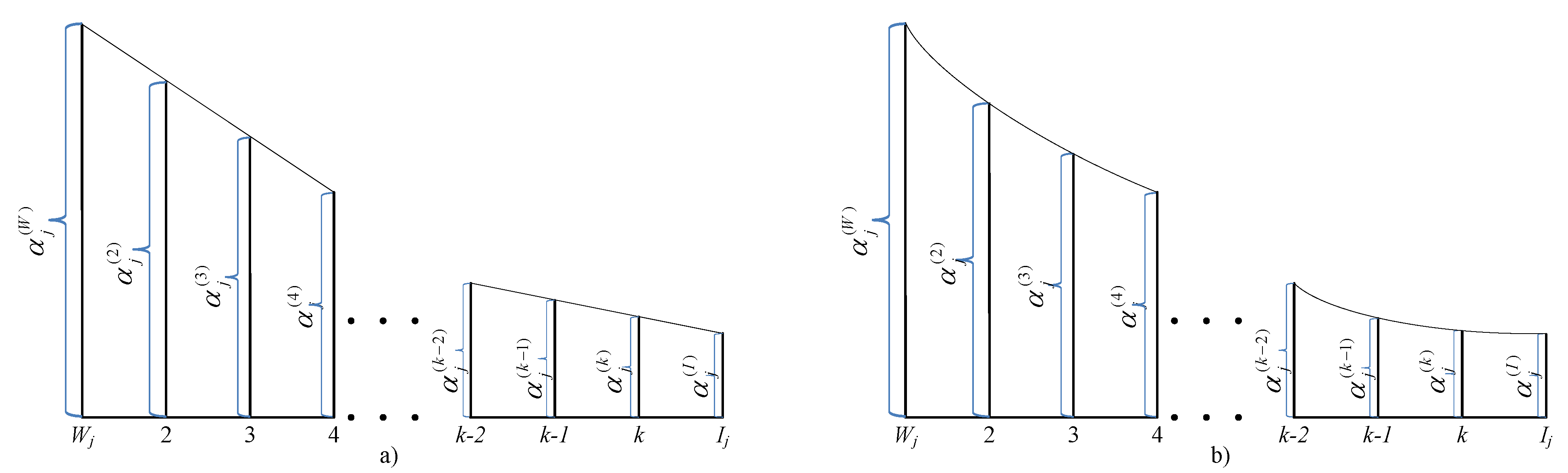
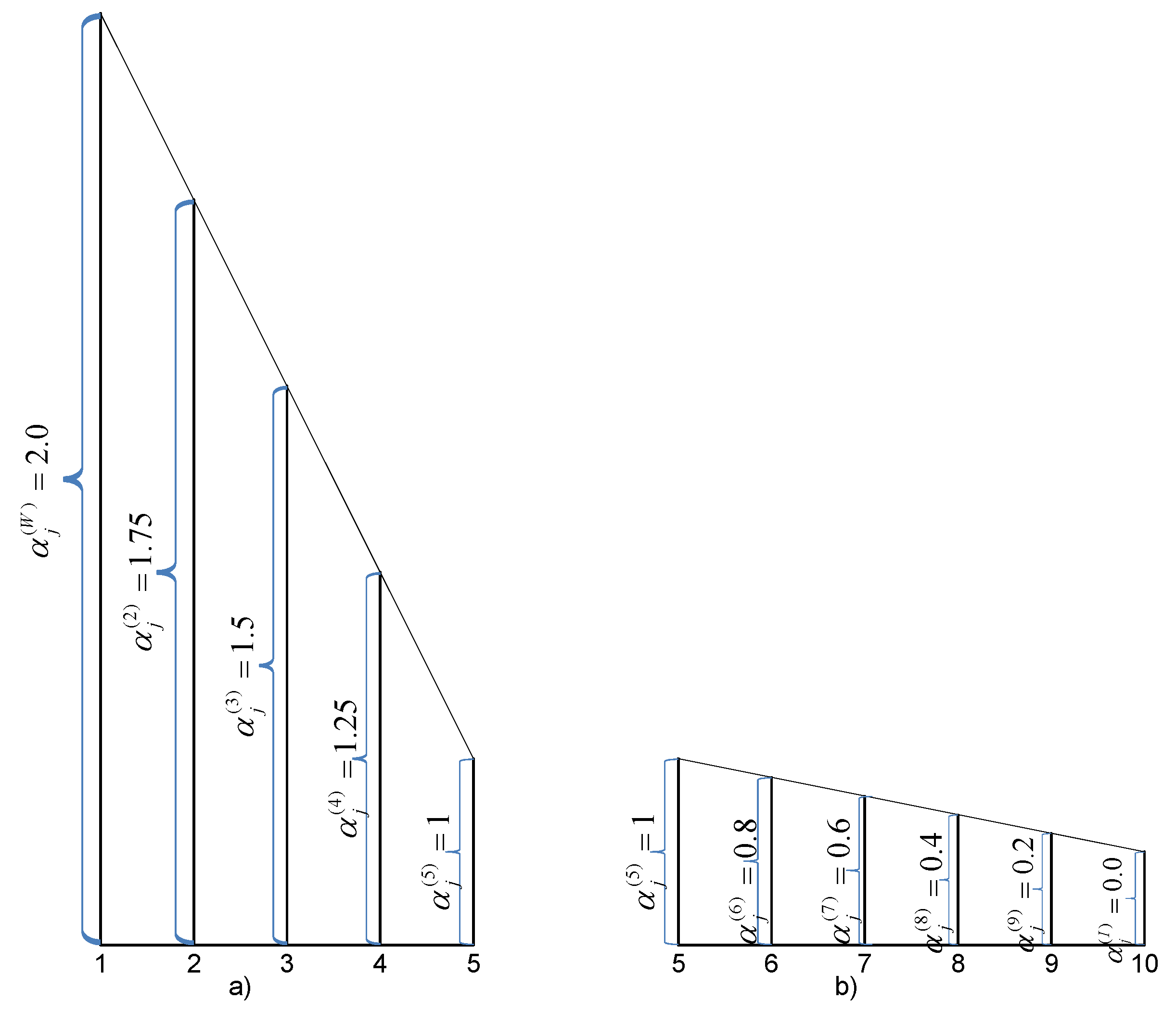
The initial decision-making matrix consists of 36 alternatives, or drivers, who are evaluated. The alternatives are marked as $A_i$ ($i=1,2,\dots ,36$). Criteria C1 and C2 are of the minimizing type, while the criteria C3, C4, and C5 are of the maximizing type. Elements of the initial matrix that refer to criteria C1 and C2 are received through measuring real indicators, while the criteria C3, C4, and C5 are evaluated by the decision-maker. For evaluating, a five-step scale is used: 1—very bad; 3—bad; 5—average; 7—good; 9—very good. The total number of evaluated drivers is 36. After forming the starting decision-making matrix, in

Table 5. The initial decision-making matrix.

Alternative	C1 (Min)	C2 (Min)	C3 (Max)	C4 (Max)	C5 (Max)
A1	28.0	0.000	7	7	5
A2	30.0	0.000	3	3	3
A3	29.5	0.000	5	5	7
A4	32.0	0.000	5	5	9
A5	28.5	0.000	5	5	9
A6	33.5	0.000	5	5	7
A7	31.5	0.000	5	5	9
A8	32.0	0.000	7	7	9
A9	33.5	0.030	3	3	9
A10	34.0	0.000	3	3	7
A11	28.5	0.000	5	5	7
A12	29.5	0.000	9	9	9
A13	33.5	0.000	9	9	7
A14	35.0	0.025	9	9	9
A15	36.5	0.000	5	5	5
A16	33.5	0.000	5	5	5
A17	31.5	0.000	3	3	3
A18	33.5	0.017	1	5	3
A19	36.0	0.000	9	9	5
A20	32.5	0.000	9	9	7
A21	33.5	0.000	9	9	3
A22	34.0	0.009	7	7	3
A23	32.5	0.000	7	7	3
A24	35.0	0.000	7	7	3
A25	35.0	0.000	7	7	5
A26	31.0	0.000	5	5	7
A27	30.5	0.000	3	3	9
A28	28.5	0.000	3	3	9
A29	31.5	0.000	9	9	7
A30	32.5	0.000	9	9	9
A31	29.5	0.000	7	7	7
A32	34.0	0.000	1	5	9
A33	31.0	0.000	3	3	5
A34	32.5	0.000	1	5	5
A35	31.0	0.000	3	3	7
A36	34.0	0.000	5	5	7

the RADERIA method algorithm is used.

Step 1.

For each criterion $C_j$ ($j=1,2,\dots ,5$) the ideal value of the alternative $I_j$ is defined, as is the anti-ideal value $W_j$ (

Table 6. Ideal and anti-ideal values of the alternatives.

Ideal/Anti-Ideal Alt.	C1	C2	C3	C4	C5
Ij	22	0	10	10	10
Wj	40	2	1	1	1

).

The values $I_j\left(22,0,10,10,10\right)$ and $W_j\left(40,2,1,1,1\right)$ are defined according to the decision-maker’s judgments based on the ideal values of the evaluating criteria.

Step 2.

In the following part, for each evaluating criterion, an advantage $I_j$ is defined compared to $W_j$. The advantage $I_j$ compared to $W_j$ is presented with ${\alpha }_j^{(I)}$ and ${\alpha }_j^{(W)}$, showing how much better the ideal alternative is than anti-ideal alternative ${\alpha }_j^{(W)}$. Value ${\alpha }_j^{(I)}$ represents a starting value for the alternative $I_j$, with which advantage ${\alpha }_j^{(W)}$ is defined. Defining values ${\alpha }_j^{(W)}$ and ${\alpha }_j^{(I)}$, the interval for standardizing all the values from the initial decision-making matrix is determined (Table 5). In our example, the following values are determined: ${\alpha }_j^{(I)}$ = 0 and ${\alpha }_j^{(W)}$ = 2. That means that all the values from the initial decision-making matrix will be standardized in the interval [0, 2].

Step 3:

In the next part, the procedure for the development of the matrix $\overline{X}={\left[{\alpha }_{ij}\right]}_{m\times n}$ is shown, in which elements ${\alpha }_{ij}$ represent the advantage of the alternative $I_j$ compared to the alternative $A_i$. In order to define the value ${\alpha }_{ij}$, for each criterion $C_j$ ($j=1,2,\dots ,5$), a unique point $e_j$ is defined (

Table 7. Defining unique points $e_j$ for the criterion $C_j$.

Criteria	Ij	${\mathit{\alpha }}_{\mathit{j}}^{(\mathit{I})}$	Wj	${\mathit{\alpha }}_{\mathit{j}}^{(\mathit{W})}$	${\mathit{e}}_{\mathit{j}}$	${\mathit{\alpha }}_{\mathit{j}}^{(\mathit{e})}$
C1	22	0	40	2	30	1
C2	0	0	2	2	0.02	1
C3	1	2	10	0	5	1
C4	1	2	10	0	5	1
C5	1	2	10	0	5	1

).

Values ${\alpha }_j^{(e)}$ from Table 7 are determined based on the decision-maker’s evaluation. Using defined unique points $e_j$ ($j=1,2,\dots ,5$) and values ${\alpha }_j^{(I)}$, ${\alpha }_j^{(W)}$ and ${\alpha }_j^{(e)}$, we can calculate values ${\alpha }_j^{(i)}$ ($i=1,2,\dots ,36$; $j=1,2,\dots ,5$) for all elements of the initial decision-making matrix. Using Expression (1), the elements ${\alpha }_{ij}$ of the matrix $\overline{X}$ are calculated. In the following part, a procedure for calculating elements of the initial matrix for the criterion C5 and alternatives A1, A2, A3, and A4 is shown:

(a)

The first group consists of the values that appear in the interval $\left[W_j,e_j\right]$ or $\left[1,5\right]$ (Figure 4a). Using Expression (1), we can define the values ${\alpha }_j^{(s)}={\alpha }_j^{(5)}=1$, ${\alpha }_j^{(s+1)}={\alpha }_j^{(W)}=2$, $e_{s+1,j}=1$ and $e_{s,j}=5$. In this way, we get the values for ${\alpha }_j^{(i)}$.

(b)

The second group consists of the values which appear in the interval $\left[e_j,I_j\right]$ or $\left[5,9\right]$ (Figure 4b). Using Expression (1), we can define the values ${\alpha }_j^{(s)}={\alpha }_j^{(10)}=0$, ${\alpha }_j^{(s+1)}={\alpha }_j^{(e)}=1$, $e_{s+1,j}=5$ and $e_{s,j}=10$. In this way, we get the values for ${\alpha }_j^{(e)}$.

$${\alpha }_3^{(7)}=0+\frac{(1-0)(7-10)}{5-10}=0.6$$

$${\alpha }_4^{(9)}=0+\frac{(1-0)(9-10)}{5-10}=0.2$$

A graphic view of the relations (${\alpha }_{C5}^{(i)}$) between $I_j$ and alternative $A_i$ ($i=1,2,\dots ,36$) is shown in Figure 4.

The shown relations also apply to the criteria C3 and C4 because the values of the alternatives on the mentioned criteria are at the same range of [1, 9]. Based on the received values ${\alpha }_j^{(i)}$, the advantage matrix of the ideal alternative compared to the alternative $A_i$ is formed.

Step 4.

The weighted advantage matrix of the ideal alternative compared to other alternatives is defined. Multiplying the matrix elements $\overline{X}$ (

Table 8. Advantage matrix of the alternative $I_j$ compared to the alternative $A_i$ ($i=1,2,\dots ,36$).

Alternative	C1	C2	C3	C4	C5
A1	0.75	0.00	0.60	0.60	1.00
A2	1.00	0.00	1.50	1.50	1.50
A3	0.94	0.00	1.00	1.00	0.60
A4	1.20	0.00	1.00	1.00	0.20
A5	0.81	0.00	1.00	1.00	0.20
A6	1.35	0.00	1.00	1.00	0.60
A7	1.15	0.00	1.00	1.00	0.20
A8	1.20	0.00	0.60	0.60	0.20
A9	1.35	1.01	1.50	1.50	0.20
A10	1.40	0.00	1.50	1.50	0.60
A11	0.81	0.00	1.00	1.00	0.60
A12	0.94	0.00	0.20	0.20	0.20
A13	1.35	0.00	0.20	0.20	0.60
A14	1.50	1.00	0.20	0.20	0.20
A15	1.65	0.00	1.00	1.00	1.00
A16	1.35	0.00	1.00	1.00	1.00
A17	1.15	0.00	1.50	1.50	1.50
A18	1.35	0.85	2.00	1.00	1.50
A19	1.60	0.00	0.20	0.20	1.00
A20	1.25	0.00	0.20	0.20	0.60
A21	1.35	0.00	0.20	0.20	1.50
A22	1.40	0.45	0.60	0.60	1.50
A23	1.25	0.00	0.60	0.60	1.50
A24	1.50	0.00	0.60	0.60	1.50
A25	1.50	0.00	0.60	0.60	1.00
A26	1.10	0.00	1.00	1.00	0.60
A27	1.05	0.00	1.50	1.50	0.20
A28	0.81	0.00	1.50	1.50	0.20
A29	1.15	0.00	0.20	0.20	0.60
A30	1.25	0.00	0.20	0.20	0.20
A31	0.94	0.00	0.60	0.60	0.60
A32	1.40	0.00	2.00	1.00	0.20
A33	1.10	0.00	1.50	1.50	1.00
A34	1.25	0.00	2.00	1.00	1.00
A35	1.10	0.00	1.50	1.50	0.60
A36	1.40	0.00	1.00	1.00	0.60

) with the weighted coefficients of the criterion, $w_j$ we get the weighted advantage matrix of the ideal alternative relative to the alternative $A_i$ (

Table 9. The weighted advantage matrix of the alternative $I_j$ compared to other alternatives.

Alternative	C1	C2	C3	C4	C5	$\mathit{Q}({\mathit{A}}_{\mathit{i}})$	Rank
A1	0.325	0.000	0.077	0.058	0.087	0.547	2
A2	0.434	0.000	0.191	0.145	0.130	0.900	25
A3	0.407	0.000	0.128	0.096	0.052	0.683	11
A4	0.521	0.000	0.128	0.096	0.017	0.762	16
A5	0.353	0.000	0.128	0.096	0.017	0.594	4
A6	0.586	0.000	0.128	0.096	0.052	0.862	20
A7	0.499	0.000	0.128	0.096	0.017	0.740	13
A8	0.521	0.000	0.077	0.058	0.017	0.672	9
A9	0.586	0.257	0.191	0.145	0.017	1.196	35
A10	0.607	0.000	0.191	0.145	0.052	0.996	33
A11	0.353	0.000	0.128	0.096	0.052	0.629	7
A12	0.407	0.000	0.026	0.019	0.017	0.469	1
A13	0.586	0.000	0.026	0.019	0.052	0.683	10
A14	0.651	0.256	0.026	0.019	0.017	0.969	29
A15	0.716	0.000	0.128	0.096	0.087	1.027	34
A16	0.586	0.000	0.128	0.096	0.087	0.897	24
A17	0.499	0.000	0.191	0.145	0.130	0.965	28
A18	0.586	0.217	0.255	0.096	0.130	1.285	36
A19	0.694	0.000	0.026	0.019	0.087	0.826	19
A20	0.542	0.000	0.026	0.019	0.052	0.639	8
A21	0.586	0.000	0.026	0.019	0.130	0.761	15
A22	0.607	0.115	0.077	0.058	0.130	0.987	32
A23	0.542	0.000	0.077	0.058	0.130	0.807	17
A24	0.651	0.000	0.077	0.058	0.130	0.915	27
A25	0.651	0.000	0.077	0.058	0.087	0.872	22
A26	0.477	0.000	0.128	0.096	0.052	0.753	14
A27	0.456	0.000	0.191	0.145	0.017	0.809	18
A28	0.353	0.000	0.191	0.145	0.017	0.706	12
A29	0.499	0.000	0.026	0.019	0.052	0.596	5
A30	0.542	0.000	0.026	0.019	0.017	0.605	6
A31	0.407	0.000	0.077	0.058	0.052	0.593	3
A32	0.607	0.000	0.255	0.096	0.017	0.977	30
A33	0.477	0.000	0.191	0.145	0.087	0.900	25
A34	0.542	0.000	0.255	0.096	0.087	0.981	31
A35	0.477	0.000	0.191	0.145	0.052	0.865	21
A36	0.607	0.000	0.128	0.096	0.052	0.884	23

).

Steps 5 and 6:

The final value of the criteria function and ranking of the alternatives is determined. Using Expression (4), we get the final values of the alternative’s criteria functions $Q(A_i)$ (Table 9). Ranking of the alternatives is done based on the values of the criteria function $Q(A_i)$. The value of the function $Q(A_i)$ shows how much further the alternative A_i is from the ideal alternative. For the alternative to be ranked as high as possible, it is desirable to have a lower value $Q(A_i)$, that is, to be as close as possible to the ideal alternative.

5. Validity of the Results

In this section of the paper, the validity of the results is shown using the RADERIA model. The sensitivity analysis is conducted through three phases: (1) In the first phase, the validity of the results is done through comparison with other multi-criteria methods; (2) the second phase implies checking the stability of the RADERIA model in dynamic conditions, that is, the resistance of the model to the rank reversal problem; and (3) the third phase represents analyzing the influence of the change of the measuring scale on ranking results.

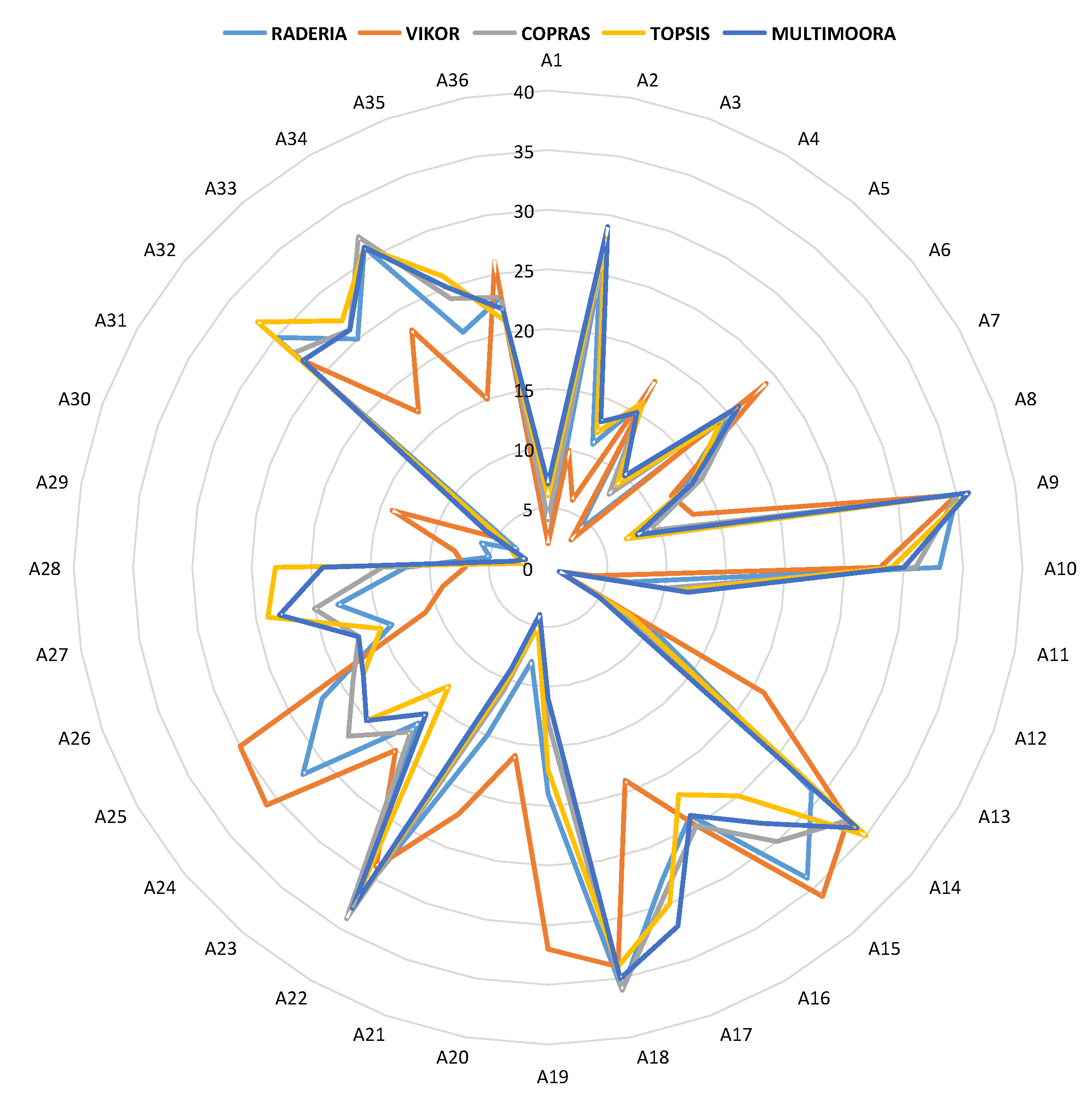
5.1. Comparison with the Other Multi-Criteria Methods

In this part of the paper, the results’ validity is shown by comparing the new RADERIA method with other traditional multi-criteria techniques. The comparison was made with the following multi-criteria models: TOPSIS [38], VIKOR (VIsekriterijumsko KOmpromisno Rangiranje) [39], MULTIMOORA (Multi-Objective Optimization by a Ratio Analysis plus the Full Multiplicative Form) [40], and COPRAS (Complex Proportional ASsessment) [41]. The same set of alternatives and the same values of the weighted criteria were used in the TOPSIS, VIKOR, MULTIMOORA, and COPRAS methods. The results of using the above-mentioned methods can be seen in Figure 5.

The ranking results show that all multi-criteria models confirm that the alternative A12 ranked first. In the VIKOR model, as well as at the RADERIA model, the alternative A1 is second-ranked. Simultaneously, the alternative A1 is fourth-ranked in the COPRAS model and sixth-ranked in the TOPIS model, while it is seventh-ranked in the MULTIMOORA model. Simultaneously, all the models suggest the set {A9, A18} as the set of the worst alternatives. Comparing the RADERIA model ranks with the other multi-criteria techniques, it can be observed that several models suggest no unique rank. The reason for having the differences in rankings is having many alternatives with not many differences between them.

To determine the relationships among the results acquired through different MCDM techniques, Spearman’s rank correlation coefficient (SCC) is used. SCC is one of the useful and significant measures for determining statistical correlation when we have ordinal variables or ranking variables. In this paper, SCC is used in order to determine the statistical importance of the difference among the rankings which were acquired through the RADERIA model and other approaches,

Table 10. Ranking correlation of the tested models.

MCDM Model	RADERIA	VIKOR	COPRAS	TOPSIS	MULTIMOORA
RADERIA	1.000	0.832	0.968	0.938	0.930
VIKOR	-	1.000	0.712	0.644	0.620
COPRAS	-	-	1.000	0.968	0.987
TOPSIS	-	-	-	1.000	0.982
MULTIMOORA	-	-	-	-	1.000

.

Despite the fact that the COPRAS, TOPSIS, and MULTIMOORA methods apply different ways of data normalization, a high correlation was achieved. Correlation with the COPRAS, TOPSIS, and MULTIMOORA models is in the interval [0.930, 0.968], while the correlation with the VIKOR model is 0.832. There are numerous studies in the literature [42,43,44,45] that show that the application of different normalization techniques can lead to rank differences in the applied MCDM techniques. This is the reason for the small correction between the ranks of the VIKOR and MULTIMOORA methods and the TOPSIS method. The VIKOR and MULTIMOORA methods apply linear normalization, while the TOPSIS method applies vector normalization; therefore, the small correlation is a consequence of the application of different normalization techniques.

The high correlation of the RADERIA method results with the results of other MCDM techniques proves the effectiveness and credibility of the RADERIA methodology. The mean SCC value for all of the models is 0.917. A lower correlation between the VKOR and RADERIA models is expected due to the specific algorithm of the VIKOR method. Namely, the VIKOR methodology takes into account the optimistic and pessimistic index when ranking alternatives. Thus, the final working alternative depends on a pessimistic and optimistic scenario, which is not the case with the RADERIA method. If the pessimistic index is eliminated with the VIKOR methodology, the results are obtained (SCC = 0.973), resulting in a significantly higher correlation with the RADERIA method. The results show that there is a high correlation of the rankings between the RADERIA model and other used techniques. According to some research [41], all the SCC values higher than 0.8 show a significantly high correlation. Because we have all the values for SCC significantly higher than 0.8 in this paper and the average value is 0.917, we can conclude that there is a high correlation between the suggested approach and other tested MCDM techniques. Based on the achieved results, we can conclude that the suggested rank is confirmed and credible.

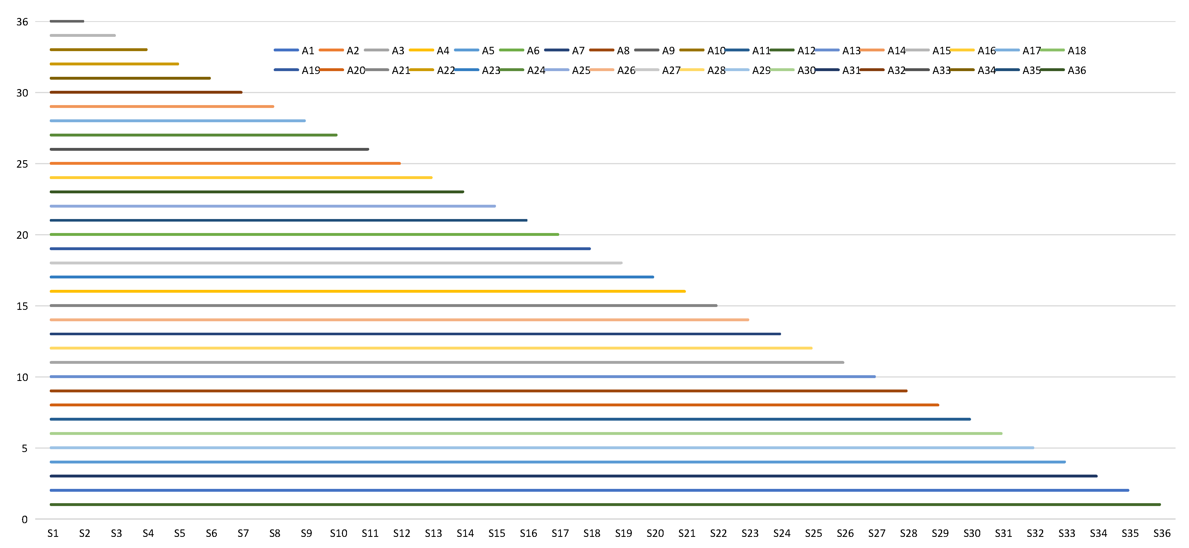
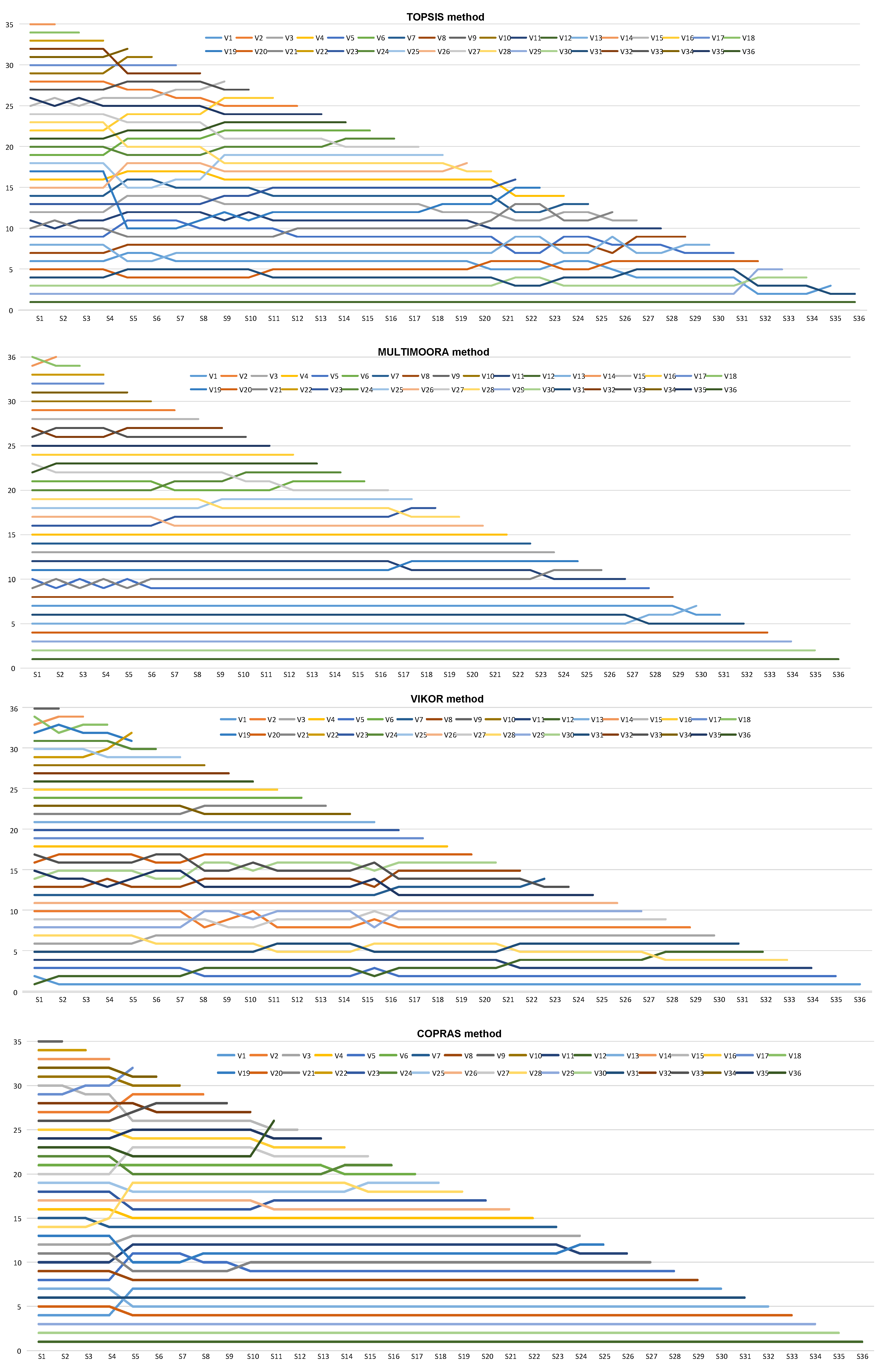
5.2. Rank Reversal Problem

One way to verify the validity of the decision-making model is to construct the dynamic matrixes and then evaluate the results given by the model in newly formed conditions. Suppose the results show some logical inconsistencies, which can be seen through unwanted alternative rankings. In that case, there might be a concern that there is a problem with the applied method’s mathematical apparatus.

To observe this problem more clearly, we shall examine the example of three candidates applying for a working position. We shall denote the candidates as A, B, and C, and we shall assume that one of the multi-criteria methods for candidate rankings was used. The applied multi-criteria model suggested the following ranking A > B > C, according to which the first candidate is the most suitable for the working position, and then candidates B and C, respectively. Then, let us assume that candidate B, who is in the second position, is replaced with a worse candidate, D. At the same time, candidates A and C are considered for the position with the same characteristics as before. It is necessary that the new set of alternatives (A, D, and C) be ranked, assuming that the criteria have exactly the same weight as before. The question is whether candidate A, after the ranking, would still be the best candidate.

The rank reversal problem was noticed for the first time by Belton and Gear [46] and they examined the use of the AHP model for ranking alternatives. They conducted simple research considering three alternatives and two criteria. They introduced the copy of a non-optimal alternative, which resulted in increasing the set of alternatives to four. After they evaluated the new set of alternatives, assuming that all the criteria were of the same weight as before, they noticed that the indication of the best alternative could change. They proved the possibility of a rank reversal in the AHP model. A few years later, Triantaphyllou and Mann [47] noticed that the rank reversal problem can occur even when a non-optimal alternative is replaced with the worse one, and not with a copy, which was the case in Belton and Gear’s experiment. Later on, many authors have shown that this problem occurs in many multi-criteria models [48,49,50,51,52,53].

Taking all the above into consideration, testing the resistance of the RADERIA model to the rank reversal problem represents a logical step to validate the results of the model, and also the recommendation of the new multi-criteria model for solving real-world problems. In this section, an experiment was carried out to evalutate the resistance of the RADERIA model to the rank reversal problem. Thirty-five scenarios were formed in the experiment, where the change of elements in the decision-making matrix was simulated. For each scenario, the number of alternatives was changed, eliminating the worst alternative from further consideration. After defining the new set of alternatives, in the newly formed conditions, the ranking of the remaining alternative was done using the RADERIA model. This experiment has two goals: (1) observing the complexity of the received result in uncertain conditions and (2) analyzing the performance of the RADERIA model in dynamic initial decision-making matrix conditions.

In the initial scenario, the worst alternative, A18, was eliminated from further consideration. The RADERIA model was applied to the new set of 35 alternatives and the new ranking was achieved (Figure 6). The new result confirms that A12 is still the best alternative, while A9 is the worst alternative. Further implementation of the presented approach allows acquiring the preferences of the remaining scenarios (Figure 6).

At the same time, the other MCDM techniques used in this paper were tested in the same conditions—TOPSIS, VIKOR, MULTIMOORA and COPRAS. In Figure 7, the results of using the TOPSIS, VIKOR, MULTIMOORA, and COPRAS models in a dynamic environment are shown.

In Figure 6, we can see that the rank reversal problem does not appear in the RADERIA model, while in TOPSIS, VIKOR, MULTIMOORA, and COPRAS models (Figure 7) the problem of rank reversal appears in many scenarios. Through all 36 scenarios in TOPSIS, VIKOR, MULTIMOORA, and COPRAS, the change in function criteria appears. That further leads to the change in the ranking of the alternatives. The rank of the best alternative (A12) does not change in the TOPSIS, MULTIMOORA, and COPRAS models. However, in the VIKOR model, after the first scenario, the alternative A12 falls to second place, after the seventh scenario, to third place, then finally in S32, it falls to fifth place. We have a similar situation with the change in the ranks of the remaining alternatives in the VIKOR model, as well as the TOPSIS, MULTIMOORA, and COPRAS models.

In the RADERIA model, during the experiment, the values of the alternatives ($Q(A_i)$) remain unchanged, so rank reversal does not happen regardless of the number of alternative changes. In the RADERIA method, the alternative A12 ranked best through all 36 scenarios which confirms the complexity and stability of the RADERIA model in a dynamic environment. Besides that, it is shown that the RADERIA model is resistant to the rank reversal of the alternatives.

5.3. Changes of the Range in Measurement Scale

In multi-criteria models, decision-makers often express their judgments using different ranges in measurement scales. Pamucar and Cirovic [42] showed that the use of different ranges in measurement scales, in certain multi-criteria models, can result in rank reversal of the alternatives. In the following part, the analysis was conducted, showing how the change of the ranges in measurement scales affects the ranking results in the RADERIA model. As stated in the previous part of the paper, for presenting values of the criteria C3, C4, and C5, a 5-point scale was used in the interval [1, 9]. From the interval [1, 9], only the odd values were used. The transformation of the range in the measurement scales was done using the following function $y=x/2+1/2$; that is how the 5-point scale was achieved in the interval [1, 5].

The results acquired using the range in the measurement scale of 1–5, show that the RADERIA method is stable and that the change of the range in the measuring scale does not lead to a change in rankings. Using the range in the interval 1–5 in the RADERIA model leads to the change of the values of the criteria functions, but these changes are not enough to change the rank of the alternatives. This experiment shows the stability of the results of the RADERIA model, recommending it for solving real-world problems.

6. Discussion of Results

To improve the complexity of the model of multi-criteria decision making [54,55,56,57,58,59], the RADERIA model is proposed based on the relation between the alternatives. Relations between the alternatives are defined according to the reference point (ideal and anti-ideal alternatives) which enables comprehensive information on alternatives and making an objective decision. The RADERIA model, as a multi-criteria model for making decisions, represents a powerful and complex tool for optimizing multiple goals. Compared to other methods, this method is simple and effective, enables easy sorting and optimization of the analyzed goals. In comparison with other multi-criteria methods, this method has an effective mathematical tool that eliminates the rank reversal problem.

The RADERIA model improves the MCDM field, introducing an algorithm that eliminates the rank reversal problem. The RADERIA method integrates three starting points for making a complex decision: (1) defining reference points (ideal and anti-ideal values); (2) determining relations between alternatives and ideal/anti-ideal values; and (3) aggregation of the alternative values for expressing the estimated distance of the alternatives compared to the ideal solution. Moreover, the results achieved through the RADERIA method are more rational because of the new approach which enables aggregation of the estimated distance alternatives from reference points. In the following part, the advantages of the RADERIA model and the reason it stands out compared to other traditional multi-criteria models are outlined:

• The new model for data normalization: The RADERIA model has a new approach for data normalization. Most MCDM techniques that are available today use a model for data normalization in which all data are converted to values in the interval [0, 1]. However, the new model for normalization, presented in this model, allows converting data from the initial decision-making matrix into any interval that is suitable for making rational decisions. This way, it facilitates making rational decisions because the new approach enables defining intervals according to the decision-maker’s judgments. For example, in this paper, all values from the initial decision-making matrix are converted into the interval [0, 2], while in other applied models (TOPSIS, VIKOR, COPRAS, and MULTIMOORA), all values are normalized into the interval [0, 1].
• The adaptivity of the RADERIA model through the model transformation for data normalization: The model for normalization of the data which is applied in the RADERIA model represents a linear model for normalization (Figure 3a), which is based on a linear function. Adaptivity of the model can be seen in its transformation into other forms of decreasing functions, for example, quadratic functions (Figure 3b). This characteristic allows the real presentation of expert judgments and making rational decisions.
• The resistance of the RADERIA model to rank reversal problem: One of the most significant disadvantages of many MCDM methods is the rank reversal problem. The question of rank reversal was noticed by Belton and Gear [46] for the first time. To this day, this issue has received great attention. Moreover, there are many studies [48,50,51] that analyze this phenomenon and show its importance in the process of making decisions. This phenomenon especially comes to expression in dynamic conditions of making decisions where the number of alternatives changes during the process of making a decision. This phenomenon can be noticed in many traditional MCDM methods. For example, the phenomenon of rank reversal is confirmed for AHP, ELECTRE (ELimination and Choice Expressing REality), TOPSIS, and PROMETHEE (Preference Ranking Organization METhod for Enrichment of Evaluations). Besides the mentioned methods, the rank reversal problem is also confirmed in this paper in MULTIMOORA, COPRAS, and VIKOR methods. However, in the same experiment, the RADERIA model shows resistance to rank reversal. Consequently, the RADERIA method shows significant stability and reliability of the results in a dynamic environment. It is also important to mention that in numerous simulations, the RADERIA method shows stability while processing a larger number of datasets. The study case also confirmed this with 36 alternatives, as examined in this paper.

In further analysis of the results, we compared the RADERIA method with other methods in the MCDM. The results showed mild deviations of the rankings compared to the examined methods (Table 10). The highest closeness of ranks is indicated with the COPRAS method. Moreover, a high correlation is shown with the TOPSIS and the MULTIMOORA models. A slightly lower correlation among the ranks can be seen in the VIKOR model with SCC = 0.832. These results were expected because the VIKOR model possesses a specific mathematical algorithm that examines the relationship between the optimistic and pessimistic results and finds a compromise between the two. The specificity of the VIKOR algorithm was also confirmed when determining correlation with other models: COPRAS–SCC = 0.712, TOPSIS–SCC = 0.644 and MULTIMOORA–SCC = 0.620. When observing an optimistic solution in VIKOR, then the correlation among the ranks increases from SCC = 0.832 to SCC = 0.966.

From the above analysis, we can conclude that the RADERIA method represents a new approach for rational decision-making that processes information on preferences in a new and original way.

The new data normalization model contributes to a realistic and stable assessment of decision-making problems. This further improves the accuracy and reliability of the results, which is especially important for solving real-world problems in various fields. As MCDM seeks to implement a reliable and rational decision-making model, the RADERIA model is the logical choice for future multi-criteria solving of problems.

7. Conclusions

The results from the conducted research and study make a double contribution, which can be seen through the possibility of acquiring experts and scientific optimal approximation. The expert contribution represents the possibility of rationalization of the costs that appear in the transportation process alone. Creating a motivational model where every driver will try to increase their engagement, on the one hand, and decrease fuel costs, on the other hand, affects the entire organization and achieves a more efficient business. This is possible if all the factors are satisfied by the drivers. Companies in developing countries, as is the case in Bosnia and Herzegovina, do not adequately understand the role and the importance of HR because they mainly invest in assets and equipment, and much less into human resources. This research should serve as one of the most important in creating evaluating and self-evaluating models for companies in Bosnia and Herzegovina.

In this paper, two innovative multi-criteria models are suggested (the LBWA model and the RADERIA model) that together form a hybrid LBWA–RADERIA multi-criteria model. The LBWA model was used for determining weighted coefficients of criteria, while the RADERIA model was used for evaluating drivers in the analyzed transportation company. The original approach for grouping criteria by importance levels in the LBWA model enables easier defining relations among criteria and maximal consistency of the results. The LBWA model is used for expressing real relations among criteria, without approximations of the expert judgments. Moreover, the LBWA model eliminates deviations of expert judgments that appear after using scales with a small range of values [37]. By eliminating this kind of problem, we also eliminate the approximation of expert judgments. This further has an impact on the distortion of the consistency of the model, i.e., distancing weighted coefficients from the optimal values. Besides the LBWA model, a new multi-criteria model for evaluating alternatives is suggested—the RADERIA model. The RADERIA model has shown a high level of flexibility and complexity of the results, which makes it recommended for solving other real problems in different areas. The proposed model is based on expert knowledge, which enables expressing expert judgments in accordance with the specificity of the observed problem. The original mathematical tool of the RADERIA model helps to convert data from the initial decision matrix into any interval, which is suitable for rational decision making. This adaptability can help managers use this methodology for making decisions in different, real situations.

In accordance with the foregoing, we can outline the importance of this paper: (1) developing the new multi-criteria methodology, the LBWA–RADERIA model, for solving real problems in the business world; (2) reviewing the new RADERIA method, which is based on the rational defining relations between the ideal and anti-ideal alternative; (3) developing the new multi-criteria model which eliminates the rank reversal problem and which offers reliable results for achieving rational decisions; and (4) developing the original universal problem for evaluating HR, which enables rational managing with human potentials in a company.

The new multi-criteria methodology, which is suggested through the RADERIA model, is validated through three phases: (1) in the first phase, comparison with the TOPSIS, VIKOR, MULTIMOORA, and COPRAS models was conducted. The results showed a high level of correlation between the results of the RADERIA model and other tested models; (2) in the second phase, testing of the RADERIA, TOPSIS, VIKOR, MULTIMOORA, and COPRAS models in dynamic conditions was conducted, that is, the resistance of the model to the rank reversal problem was tested. The testing showed that the RADERIA model eliminates the rank reversal problem, while other models (TOPSIS, VIKOR, MULTIMOORA, and COPRAS) do not give reliable results in dynamic conditions; and (3) in the third phase, the validity of the results was executed in the case when there was a change in the measurement scale of the qualitative criteria. The RADERIA method showed complexity in the case of different measurement scales. It showed that a slight change occurs in the values of the criteria functions, but the rankings remain the same. The stability of the RADERIA method is confirmed, making it recommendable for use in future research to address multi-criteria problems.

The directions of future research should be directed toward the implementation of the RADERIA method for solving other real problems. Additionally, one of the directions of future research should be the extension of the RADERIA method in a fuzzy and rough environment [60], where the application of linguistic variables would allow rational expression of human judgments. In addition, the RADERIA method can be used with other methods for determining the weight of the criteria. It is possible to generate random data and perform a correlation study in order to prove the robustness of the RADERIA model additionally. This could be a direction for future research, also.

References

1. Stević, Ž.; Pamučar, D.; Kazimieras Zavadskas, E.; Ćirović, G.; Prentkovskis, O. The selection of wagons for the internal transport of a logistics company: A novel approach based on rough BWM and rough SAW methods. Symmetry 2017, 9, 264. [Google Scholar] [CrossRef] [Green Version]
2. Koskinen, P.; Hilmola, O.P. Supply chain challenges of North-European paper industry. Ind. Manag. Data Syst. 2008, 108, 208–227. [Google Scholar] [CrossRef]
3. Guasch, J.L. Inventories and logistic costs in developing countries: Levels and determinants, a red flag on competitiveness and growth. Rev. Competencia Prop. Intelect. 2005, 1, 1–27. [Google Scholar]
4. Rantasila, K.; Ojala, L. Measurement of national-level logistics costs and performance. In Transport Forum Discussion Paper; International Transport Forum: Paris, France, 2012. [Google Scholar]
5. Borzacchiello, M.T.; Torrieri, V.; Nijkamp, P. An operational information systems architecture for assessing sustainable transportation planning: Principles and design. Eval. Program Plan. 2009, 32, 381–389. [Google Scholar] [CrossRef] [PubMed] [Green Version]
6. Radović, D.; Stević, Ž.; Pamučar, D.; Zavadskas, E.; Badi, I.; Antuchevičiene, J.; Turskis, Z. Measuring performance in transportation companies in developing countries: A novel rough ARAS model. Symmetry 2018, 10, 434. [Google Scholar] [CrossRef] [Green Version]
7. Yusifov, F.; Alguliyev, R.; Aliguliyev, R. Multi-criteria Evaluation + Positional Ranking Approach for Candidate Selection in E-voting. Decis. Mak. Appl. Manag. Eng. 2019, 2, 65–80. [Google Scholar]
8. Stojić, G.; Sremac, S.; Vasiljković, I. A fuzzy model for determining the justifiability of investing in a road freight vehicle fleet. Oper. Res. Eng. Sci. Theory Appl. 2018, 1, 62–75. [Google Scholar] [CrossRef]
9. Ghiani, G.; Laporte, G.; Musmanno, R. Introduction to Logistics Systems Planning and Control; John Wiley & Sons: New York, NY, USA, 2004. [Google Scholar]
10. Liu, F.; Aiwu, G.; Lukovac, V.; Vukic, M. A multi-criteria model for the selection of the transport service provider: A single valued neutrosophic DEMATEL multi-criteria model. Decis. Mak. Appl. Manag. Eng. 2018, 1, 121–130. [Google Scholar] [CrossRef]
11. Ibrahimović, F.I.; Kojić, S.L.; Stević, Ž.R.; Erceg, Ž.J. Making an investment decision in a transportation company using an integrated FUCOM-MABAC model. Tehnika 2019, 74, 577–584. [Google Scholar] [CrossRef] [Green Version]
12. Savković, T.; Miličić, M.; Pitka, P.; Milenković, I.; Koleška, D. Evaluation of the eco-driving training of professional truck drivers. Oper. Res. Eng. Sci. Theory Appl. 2019, 2, 15–26. [Google Scholar] [CrossRef] [Green Version]
13. Zavalko, A. Applying energy approach in the evaluation of eco-driving skill and eco-driving training of truck drivers. Transp. Res. Part D Transp. Environ. 2018, 62, 672–684. [Google Scholar] [CrossRef]
14. Despić, D.; Bojović, N.; Kilibarda, M.; Kapetanović, M. Assessment of efficiency of military transport units using the DEA and SFA methods. Vojnoteh. Glas. Mil. Tech. Cour. 2019, 67, 68–92. [Google Scholar] [CrossRef]
15. Boyce, W.S. Does truck driver health and wellness deserve more attention? J. Transp. Health 2016, 3, 124–128. [Google Scholar] [CrossRef]
16. Hashemkhani Zolfani, S.; Maknoon, R.; Zavadskas, E.K. An introduction to prospective multiple attribute decision making (PMADM). Technol. Econ. Dev. Econ. 2016, 22, 309–326. [Google Scholar] [CrossRef]
17. Dobrosavljević, A.; Urošević, S. Analysis of business process management defining and structuring activities in micro, small and medium–sized enterprises. Oper. Res. Eng. Sci. Theory Appl. 2019, 2, 40–54. [Google Scholar] [CrossRef]
18. Pamučar, D.S.; Savin, L.M. Multiple-criteria model for optimal off-road vehicle selection for passenger transportation: BWM-COPRAS model. Vojnoteh. Glas. Mil. Tech. Cour. 2020, 68, 28–64. [Google Scholar] [CrossRef]
19. Gürbüz, T.; Albayrak, Y.E. An engineering approach to human resources performance evaluation: Hybrid MCDM application with interactions. Appl. Soft Comput. 2014, 21, 365–375. [Google Scholar] [CrossRef]
20. Ellinger, A.E.; Ellinger, A.D. Leveraging human resource development expertise to improve supply chain managers′ skills and competencies. Eur. J. Train. Dev. 2014, 38, 118–135. [Google Scholar] [CrossRef]
21. Dubey, R.; Gunasekaran, A. The role of truck driver on sustainable transportation and logistics. Ind. Commer. Train. 2015, 47, 123–134. [Google Scholar] [CrossRef]
22. Klumpp, M.; Abidi, H. Competence Evaluation and Management in Logistics. Prod. Oper. Manag. 2013, 22, 3–6. [Google Scholar]
23. Wu, Y.J.; Hou, J.L. An employee performance estimation model for the logistics industry. Decis. Support Syst. 2010, 48, 568–581. [Google Scholar] [CrossRef]
24. Chang, Y.W. Employee performance appraisal in a logistics company. Open J. Soc. Sci. 2015, 3, 47. [Google Scholar] [CrossRef] [Green Version]
25. Jhawar, A.; Garg, S.K.; Khera, S.N. Modelling and evaluation of investment strategies in human resources for logistics improvement. Int. J. Simul. Process. Model. 2016, 11, 36–50. [Google Scholar] [CrossRef]
26. Kampf, R.; Ližbetinová, L. The identification and development of talents in the environment of logistics companies. Naše More Znan. Stručni Časopis Za More I Pomor. 2015, 62, 139–142. [Google Scholar] [CrossRef]
27. Qu, Q.; Wang, W.; Tang, M.; Lu, Y.; Tsai, S.B.; Wang, J.; Yu, C.L. A Performance Evaluation Study of Human Resources in Low-Carbon Logistics Enterprises. Sustainability 2017, 9, 632. [Google Scholar] [CrossRef] [Green Version]
28. Badi, I.; Abdulshahed, A.; Shetwan, A.; Eltayeb, W. Evaluation of solid waste treatment methods in Libya by using the analytic hierarchy process. Decis. Mak. Appl. Manag. Eng. 2019, 2, 19–35. [Google Scholar] [CrossRef]
29. Xin, L.; An-quan, Z.; Man-hong, K.; Zhong-rong, T. On the application of fuzzy comprehensive appraisal in human capital evaluation of logistics enterprises. In Proceedings of the 2009 16th International Conference on Industrial Engineering and Engineering Management, Beijing, China, 21–23 October 2009; pp. 2012–2015. [Google Scholar]
30. Li, B.Z.; Wang, Y.; Bi, R. Research on evaluation index system of logistics talents based on ANP. J. Tianjin Univ. Technol. 2009, 4. Available online: https://en.cnki.com.cn/Article_en/CJFDTotal-TEAR200904021.htm (accessed on 15 April 2021).
31. Yue, S. The application of Analytic hierarchy Process in Logistics Enterprises Personnel Evaluation. In Proceedings of the 2008 IEEE International Conference on Automation and Logistics, Qingdao, China, 1–3 September 2008; pp. 2608–2613. [Google Scholar]
32. Samad, S. Examining the Predictors of Employee Work Outcomes—Case Study in Logistics Companies. J. Adv. Nat. Appl. Sci. Anas 2012, 6, 723–730. [Google Scholar]
33. Kucharčíková, A.; Mičiak, M. The application of human capital efficiency management towards the increase of performance and competitiveness in an enterprise operating in the field of distribution logistics. Naše More Znan. Stručničasopisza More Ipomorstvo 2018, 65, 276–283. [Google Scholar] [CrossRef] [Green Version]
34. Karabasevic, D.; Popovic, G.; Stanujkic, D.; Maksimovic, M.; Sava, C. An approach for hotel type selection based on the single-valued intuitionistic fuzzy numbers. Int. Rev. 2019, 7–14. Available online: https://www.ceeol.com/search/article-detail?id=852707 (accessed on 15 April 2021). [CrossRef] [Green Version]
35. Zizovic, M.; Pamucar, D. New model for determining criteria weights: Level Based Weight Assessment (LBWA) model. Decis. Mak. Appl. Manag. Eng. 2019, 2, 126–137. [Google Scholar] [CrossRef]
36. Naeini, A.B.; Mosayebi, A.; Mohajerani, N. A hybrid model of competitive advantage based on Bourdieu capital theory and competitive intelligence using fuzzy Delphi and ism-gray Dematel (study of Iranian food industry). Int. Rev. 2019, 21–35. Available online: https://www.ceeol.com/search/article-detail?id=852716 (accessed on 15 April 2021).
37. Dimić, S.; Ljubojević, S. Decision making model in forest road network management. Vojnoteh. Glas. Mil. Tech. Cour. 2019, 67, 93–115. [Google Scholar] [CrossRef]
38. Hwang, C.L.; Yoon, K. Multiple Attribute Decision Making: Methods and Applications; Springer: New York, NY, USA, 1981. [Google Scholar]
39. Opricovic, S. Multiobjective Optimization in River Basin Development. Water Resour. Res. 1980, 16, 14–20. [Google Scholar]
40. Brauers, W.K.M.; Zavadskas, E.K. Project management by MULTIMOORA as an instrument for transition economies. Technol. Econ. Dev. Econ. 2010, 16, 5–24. [Google Scholar] [CrossRef]
41. Zavadskas, E.K.; Kaklauskas, A.; Turskis, Z.; Tamošaitien, J. Selection of the effective dwelling house walls by applying attributes values determined at intervals. J. Civ. Eng. Manag. 2008, 14, 85–93. [Google Scholar] [CrossRef] [Green Version]
42. Pamucar, D.; Cirovic, G. The selection of transport and handling resources in logistics centres using Multi-Attributive Border Approximation area Comparison (MABAC). Expert Syst. Appl. 2015, 42, 3016–3028. [Google Scholar] [CrossRef]
43. Petrović, G.; Mihajlović, J.; Ćojbašić, Ž.; Madić, M.; Marinković, D. Comparison of three fuzzy MCDM methods for solving the supplier selection problem. Facta Univ. Ser. Mech. Eng. 2019, 17, 455–469. [Google Scholar] [CrossRef]
44. Zolfani, S.H.; Yazdani, M.; Pamucar, D.; Zarate, P. A VIKOR and TOPSIS focused reanalysis of the MADM methods based on logarithmic normalization. Facta Univ. Ser. Mech. Eng. 2020, 18, 341–355. [Google Scholar]
45. Bozanic, D.; Randjelovic, A.; Radovanovic, M.; Tesic, D. A hybrid LBWA-IR-MAIRCA multi-criteria decision-making model for determination of constructive elements of weapons. Facta Univ. Ser. Mech. Eng. 2020, 18, 399–418. [Google Scholar] [CrossRef]
46. Belton, V.; Gear, A.E. On a Short-Coming of Saaty′s Method of Analytic Hierarchies. Omega 1983, 11, 228–230. [Google Scholar] [CrossRef]
47. Triantaphyllou, E.; Mann, S.H. An Examination of the Effectiveness of Multi-Dimensional Decision-Making Methods: A Decision-Making Paradox. Int. J. Decis. Support Syst. 1989, 5, 303–312. [Google Scholar] [CrossRef]
48. Triantaphyllou, E. Multi-Criteria Decision Making: A Comparative Study; Kluwer Academic Publishers (Now Springer): Dordrecht, The Netherlands, 2000; p. 320. [Google Scholar]
49. Saaty, T.L. Making and validating complex decisions with the AHP/ANP. J. Syst. Sci. Syst. Eng. 2005, 14, 1–36. [Google Scholar] [CrossRef]
50. Kujawski, E. A reference-dependent regret model for deterministic tradeoff studies. Syst. Eng. 2005, 8, 119–137. [Google Scholar] [CrossRef] [Green Version]
51. Leskinen, P.; Kangas, J. Rank reversals in multi-criteria decision analysis with statistical modeling of ratio-scale pairwise comparisons. J. Oper. Res. Soc. 2005, 56, 855–861. [Google Scholar] [CrossRef]
52. Ishizaka, A.; Lusti, M. How to derive priorities in AHP: A comparative study. Cent. Eur. J. Oper. Res. 2006, 14, 387–400. [Google Scholar] [CrossRef] [Green Version]
53. Zahir, S. Normalisation and rank reversals in the additive analytic hierarchy process: A new analysis. Int. J. Oper. Res. 2009, 4, 446–467. [Google Scholar] [CrossRef]
54. Opricovic, S.; Tzeng, G.-H. Extended VIKOR Method in Comparison with Outranking Methods. Eur. J. Oper. Res. 2007, 178, 514–529. [Google Scholar] [CrossRef]
55. Qin, J.; Liu, X.; Pedrycz, W. An extended TODIM multi-criteria group decision making method for green supplier selection in interval type-2 fuzzy environment. Eur. J. Oper. Res. 2017, 258, 626–638. [Google Scholar] [CrossRef]
56. Banaeian, N.; Mobli, H.; Fahimnia, B.; Nielsen, I.E.; Omid, M. Green supplier selection using fuzzy group decision making methods: A case study from the agri-food industry. Comput. Oper. Res. 2018, 89, 337–347. [Google Scholar] [CrossRef]
57. Kushwaha, D.K.; Panchal, D.; Sachdeva, A. Risk analysis of cutting system under intuitionistic fuzzy environment. Rep. Mech. Eng. 2020, 1, 162–173. [Google Scholar] [CrossRef]
58. Fan, Z.P.; Zhang, X.; Chen, F.D.; Liu, Y. Extended TODIM method for hybrid multiple attribute decision making problems. Knowl. Based Syst. 2013, 42, 40–48. [Google Scholar] [CrossRef]
59. Mihajlović, J.; Rajković, P.; Petrović, G.; Ćirić, D. The Selection of the Logistics Distribution Center Location Based on MCDM Methodology in Southern and Eastern Region in Serbia. Oper. Res. Eng. Sci. Theory Appl. 2019, 2, 72–85. [Google Scholar] [CrossRef]
60. Precup, R.-E.; Preitl, S.; Petriu, E.; Bojan-Dragos, C.-A.; Szedlak-Stinean, A.-I.; Roman, R.-C.; Hedrea, E.-L. Model-Based Fuzzy Control Results for Networked Control Systems. Rep. Mech. Eng. 2020, 1, 10–25. [Google Scholar] [CrossRef]
Figure 1. Multi-criteria methodology for evaluating drivers.
Mathematics 09 00976 g001
Figure 2. The LBWA model algorithm.
Mathematics 09 00976 g002
Figure 3. The advantage ( α j ( i ) ) of the ideal alternative I j compared to the anti-ideal alternative W j .
Mathematics 09 00976 g003
Figure 4. Relations of the alternative I j compared to the alternative A i ( i = 1 , 2 , , 36 ) for the criterion C5.
Mathematics 09 00976 g004
Figure 5. Comparison of the RADERIA method with other multi-criteria methods.
Mathematics 09 00976 g005
Figure 6. Dynamic matrix—the RADERIA model.
Mathematics 09 00976 g006
Figure 7. Dynamic matrix—TOPSIS, VIKOR, MULTIMOORA and COPRAS models.
Mathematics 09 00976 g007