Abstract
Ambiguous and uncertain facts can be handled using a hesitant 2-tuple linguistic set (H2TLS), an important expansion of the 2-tuple linguistic set. The vagueness and uncertainty of data can be grabbed by using aggregation operators. Therefore, aggregation operators play an important role in computational processes to merge the information provided by decision makers (DMs). Furthermore, the aggregation operator is a potential mechanism for merging multisource data which is synonymous with cooperative preference. The aggregation operators need to be studied and analyzed from various perspectives to represent complex choice situations more readily and capture the diverse experiences of DMs. In this manuscript, we propose some valuable operational laws for H2TLS. These new operational laws work through the individual aggregation of linguistic words and the collection of translation parameters. We introduced a hesitant 2-tuple linguistic weighted average (H2TLWA) operator to solve multi-criteria group decision-making (MCGDM) problems. We also define hesitant 2-tuple linguistic Bonferroni mean (H2TLBM) operator, hesitant 2-tuple linguistic geometric Bonferroni mean (H2TLGBM) operator, hesitant 2-tuple linguistic Heronian mean (H2TLHM) operator, and a hesitant 2-tuple linguistic geometric Heronian mean (H2TLGHM) operator based on the novel operational laws proposed in this paper. We define the aggregation operators for addition, subtraction, multiplication, division, scalar multiplication, power and complement with their respective properties. An application example and comparison analysis were examined to show the usefulness and practicality of the work.
1. Introduction
Multi-criteria decision making (MCDM) is an immensely important and common practice in our everyday life. In the literature, countless decision-making techniques and their extensions have been proposed, for example, the technique for order of preference by similarity to ideal solution (TOPSIS) [1,2,3], VIKOR [4,5,6,7], Preference Ranking Organization Method for enrichment of evaluations (PROMETHEE II) [8,9,10], analytic hierarchy process (AHP) [11,12,13], analytic network process (ANP) [14,15,16], the complex proportional assessment (COPRAS) [17,18], ELECTRE [19,20,21], the characteristic objects method (COMET) [22,23,24,25,26,27], best–worst method (BWM) [28,29,30], among others [31]. With the advancement of society, some new methodologies for capturing cognitive uncertainty among DMs in addressing the complexity of management decisions are generally required. MCDM is an autonomous discipline concerned with prioritizing the appropriate alternative(s), subject to a range of parameters or characteristics that may be valid or ambiguous.
The fuzzy set theory was proposed by Zadeh [32] in 1965 to tackle imprecise and ambiguous circumstances. A fuzzy set has been described in some universe of discourse, each element of which is associated with the degree of membership. Fuzzy set theory is developed to find unfaithfulness and uncertainty to demonstrate the human mind in computerized reasoning. The significance of such a theory is expanding step by step in the field of an expert system. Various types of fuzzy knowledge have been commonly used to address MCDM problems. As a result, fuzzy set theory and its generalization have emerged as a possible field of interdisciplinary study. Sometimes, the DMs dealing with an ambiguous problem cannot interpret their understanding with the help of a single term because they consider multiple terms all at once. Therefore, in order to overcome this issue, hesitant fuzzy sets (HFSs) theory [33] was introduced, which can be used in MCDM problems. Various types of fuzzy knowledge have been commonly used to address MCDM problems. Consequently, the fuzzy set theory and its generalization emerged as a potential field of interdisciplinary study. As a rationalization of Zadeh’s fuzzy sets, fuzzy logic combines linguistic variables in the dynamic display system. The need for linguistic variables was felt when the DMs preferred variable values in words rather than numbers. Zadeh himself introduced linguistic variables in 1975 [34]. In a characteristic or natural language, the linguistic variable carries its values in the form of words or phrases.
The analysis of the different linguistic extensions and the fuzzy linguistic structure and speculations shows that, for the most part, that the modeling of linguistic information is exceptionally constrained since it depends on the causal inference of single and extremely straight words, which should incorporate and exhibit the linguistic variable data provided by the DMs. Linguistic variables provide an updated and accurate source of imprecise or uncertain qualitative knowledge but have certain limitations, like the limitation of the number of linguistic terms, multi-faceted calculational existence, and the absence of accuracy and adversity in the estimation procedure [35,36]. In order to control these shortcomings, a 2-tuple proportional model [37], a 2-tuple linguistic model [38], a virtual linguistic model [39], and a hesitant fuzzy linguistic term sets [40] were suggested. In the past, many scholars introduced a variety of linguistic term models in their research, for example, the symbolic model [41,42], the semantic model [43,44], and the model formed on linguistic 2-tuple. Three such models were introduced in the year 2000 by Herrera and Martinez. The extension principal is considered as basic for the semantic model, and the symbolic model is based on computations using the index of linguistic terms.
Several other similar models are carried by the 2-tuple family, so that based on the principle of symbolic translation, the 2-tuple fuzzy linguistic representation model was built in [45]. The fundamental belief of this model is to set the correct numerical scale to make adjustments between linguistic 2-tuple and numerical consistency. Herrera and Martinez (2000) suggested the 2-tuple linguistic model that guaranteed consistency in consistently distributing LTs with the same precision. Wang and Hao [37] developed the proportional 2-tuple fuzzy linguistic representation model in addition to the Herrera and Martinez model to remove the drawback of 2-tuple linguistic model. Furthermore, the notation of a hesitant 2-tuple linguistic set introduced by Wei and Liao [46] to make the computation of hesitant fuzzy linguistic term sets (HFLTS) [40] without information loss and built up several new operators to accumulate HFLTS from different LTSs. The hesitant 2-tuple linguistic data model presented by Beg and Rashid [47] in 2016 provides a linguistic and computational framework for coping with the situation in which experts evaluate an alternative under linguistic terms and feel somewhat hesitant to demonstrate its possible linguistic translation. Faizi et al. [48,49] first introduced an outranking approach based on the ELECTRE method and then developed the TODIM approach for solving MCGDM problems in a hesitant 2-tuple linguistic environment.
DMs usually focus on consolidating the effect of different criteria. Addressing the basic situation, Bonferroni [50] presented the Bonferroni mean (BM) operator as a mean type accumulation operator, which not only represents the correlation of the attributes entered, but can also minimize mistakes in some compound circumstances. Additionally, the Bonferroni mean operator for H2TLSs has been introduced in [51]. The Heronian mean (HM) [52] is another form of decision-making operator that can also independently express the interrelationships between input data. HM is beneficial in different application areas, including decision making and data mining. From the definition of BM and HM operators, the BM operator indicates the correlation between different criteria and for . In contrast, the HM operator accounts for the interaction between criteria and pays close attention to the aggregated input data. HM indicates the interaction between an attribute and itself.
Aggregation is an important step in various types of fuzzy information decision-making methods which use aggregation operators in the last steps of the algorithm. Many aggregation operators play an important role in the aggregation process throughout MCDM problems. Many t-norms and t-conorms can be chosen for the computational analysis of linguistic knowledge. Several researchers have developed multiple aggregation operators to deal with their problems, i.e., Xunjie and Xu [53] developed aggregation operators for linguistic terms; Wang et al. [51] defined the H2TLPWA (hesitant 2-tuple linguistic prioritized weighted averaging) operator, H2TLPWG (hesitant 2-tuple linguistic prioritized weighted geometric) aggregation operator and H2TLCG (hesitant 2-tuple linguistic correlated geometric) aggregation operators for H2TLSs. Faizi et al. introduced an additive consistency-based approach with hesitant 2-tuple linguistic preference relation in [54].
We can see from the whole discussion that the MCGDM with hesitant 2-tuple linguistic information is a hot topic and has been investigated by many scholars. In this paper, we are concerned with group decision making in a hesitant 2-tuple linguistic environment. In particular, we are interested in the role that the proposed operators for H2TLSs might play in enhancing group decision making. In part, this has been motivated by our recent work [48,49], indicating the importance of H2TLSs in real-life problems. To show the applicability of the proposed operational laws for H2TLSs, we introduced a method to solve the problems of MCGDM by using the proposed H2TLWA, H2TLBM, H2TLGBM, H2TLHM and H2TLGHM operators. These operations can prevent operational results beyond the boundary of the LTSs and translation parameters and hold the likelihood information complete after operations. To show the efficiency of the proposed MCGDM method, we apply the method to solve a numerical example concerning selecting the best investment opportunity for a finance house in Pakistan. Finally, a comparative study of the proposed approach with the existing ones is conducted to illustrate the application and superiority of the proposed method.
The remainder of the paper is sorted out as follows: Section 2 addresses some of the fundamentals applicable to the proposed research. Section 3 establishes new operational laws for H2TLS along with their properties. The H2TLWA, H2TLBM, H2TLGBM, H2TLHM, and H2TLGHM operators are also defined in the same section. In Section 4, a realistic example is used to illustrate the efficacy of the proposed novel operational laws by addressing the MCGDM problem. The results are aggregated using the proposed H2TLWA, H2TLBM and H2TLHM operators. Section 5 draws some conclusions and outlines some of the research directions for H2TLS.
2. Preliminaries
This section comprises fundamental notions of LTSs, HFS, H2TLSs and a 2-tuple linguistic representation model.
Definition 1.
The linguistic term set with odd cardinality is indicated by where each displays a probable value for a linguistic variable. The properties for S can be defined as follows:
- 1.
- Negation operator: , such that
- 2.
- Ordered set: . Therefore, the following operators exist:
- a
- Maximization operator: if
- b
- Minimization operator: if
Definition 2.
Let X be a fixed defined set, h is a function that, when related to set X, returns a subset of values in called HFS on X.
Definition 3
([40]). Let be a linguistic term set, an HFLTS () is an arranged limited subset of the continuous linguistic terms of S. In mathematical form, where the possible degree of the linguistic variable x is denoted by to the linguistic term set S. is also called a hesitant fuzzy linguistic element (HFLE).
Definition 4.
Let represent a linguistic term set and the result of a symbolic aggregation operation represented by , then the 2-tuple that exhibits the equivalent information to β is obtained with the function as
is used to represent the inverse of △ which can be defined as
Definition 5
([47]). Assume that X is a fixed defined set and S be the linguistic term set as described earlier, an expression H given by defined an H2TLS in X. The hesitant 2-tuple linguistic representation model represents the hesitant linguistic information by means as a 2-tuple, , where is the linguistic label and α is an ordered finite subset of that represents the possible symbolic translations of . It is noted that the cardinality of α may be different for each x. In particular, if there is a single element in X, then H is referred to as an H2TLE, which can be denoted by .
Definition 6.
For a hesitant 2-tuple linguistic element where for we define and Clearly, is a finite subset of . Similarly, we can prove that where round and where
Definition 7.
Let be H2TLSs, where for , then the score function for H2TLTSs is defined as
where for . The following comparison analysis holds for the score function of H2TLEs.
Definition 8.
For any two H2TLEs, and
- 1.
- iff
- 2.
- iff
Definition 9.
For a hesitant 2-tuple linguistic element, , where for we define and . It can be easily observed that implies .
Definition 10
([53]). Let be an LTS, then the corresponding information to the membership degree expressed by the linguistic variable is obtained with the function defined by . The corresponding inverse function is defined as .
Definition 11.
Let be the set of parameter values of an H2TLS, then we define a function where and . Furthermore, the membership degree that shows corresponding information to parameter values of H2TLS, as obtained with the inverse function where
3. Novel Operational Laws for H2TLSs
In the course of the most recent couple of decades, we used operational laws to aggregate the H2TLSs that deal with linguistic terms and translation parameters as a single term, as discussed in the introduction. There is a need to define some new aggregation operators which deal with the H2TLS in a different way. Two similar transformation functions have been implemented in Definitions 1 and 2, on the basis of which some new operational laws for H2TLSs can be defined, including addition, subtraction, multiplication, division, multiplication of scalers, power and complement.
Definition 12.
Let be an H2TLTS, where , and let and , , , be two H2TLTEs while are symbolic translation parameters of H2TLEs and is a real number, then:
- 1.
- 2.
- 3.
- 4.
- 5.
- 6.
- 7.
Theorem 1.
Let be a linguistic term set, and be two H2TLTSs. Then, for real numbers , we have:
Proof.
Here, 1 and 2 are obvious.
3.
,
4.
5.
6.
7.
8.
9.
10.
11.
12.
☐
Definition 13.
Let be a set of n H2TLSs where for and is the weight vector with such that , then the hesitant 2-tuple linguistic fuzzy weighted average (H2TLWA) operator is defined as
Definition 14.
Let be a set of H2TLSs where for } and is the weight vector with such that , then the Boneferri mean operator for H2TLSs is defined as
and the geometric Bonferroni mean as
Theorem 2.
Let with be set of n H2TLSs as mentioned previously. Then, some characteristics of the H2TLBM operator are shown below.
1. Commutativity: If is any permutation of then:
Proof.
Since is any permutation of then:
☐
2. Boundedness: Let be a set of n H2TLSs where for then:
where and for .
Proof.
Due to for we can obtain:
☐
3. Monotonicity: Let and be two sets of n H2TLSs, that satisfy for then:
Proof.
If H and satisfy for it implies that:
☐
Definition 15.
Let be a set of H2TLSs where for then the Heronian mean for H2TLSs using novel operational laws is defined as
and the geometric Heronian mean for H2TLSs as
Theorem 3.
Let with be a set of n H2TLSs. Then, some characteristics of the H2TLHM operator are shown below.
1. Commutativity: If is any permutation of , then
Proof.
Since is any permutation of H, therefore, we can obtain:
☐
2. Boundedness: Let be set of n H2TLSs, then:
where and for .
Proof.
Due to for we can obtain:
☐
3. Monotonicity: Let and be two sets of n H2TLSs, that satisfy for then:
Proof.
If H and satisfy for then:
☐
4. Let be a set of n H2TLSs, then we can get
Proof.
From the Definition 15, we can obtain:
☐
An Approach to MCGDM Using H2TLEs
Here, we construct a MCGDM approach with H2TL information. For an MCGDM problem with H2TLSs, let indicates a set of alternatives and indicates a set of criteria. Let the criteria weight vector be given by where . Let be a set of DMs with a weight vector where Let be p evaluation matrices provided by DMs, where is an H2TLE indicating the preference value of alternative under the criteria . The proposed MCGDM approach can be categorized as follows (see Figure 1):
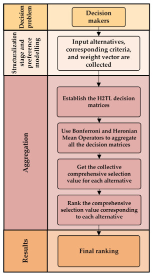
Figure 1.
Framework containing the proposed MCGDM approach with H2TL information.
- Step 1:
- Establish the H2TL decision matrices with the help of DMs ;
- Step 2:
- Use the novel operational laws to aggregate all the decision matrices provided by the DMs to get the aggregated matrix ;
- Step 3:
- Aggregate to obtain the collective comprehensive selection value for each alternative using H2TLWA, H2TLBM, H2TLGBM, H2TLHM and H2TLGHM operators;
- Step 4:
- Rank the comprehensive selection value corresponding to each alternative by computing the score values using Equation (1) and choose the best alternative , where
4. Numerical Example on an Investment Problem
Suppose a finance house is in place that needs to invest capital in the best way possible [47,48,49]. The money is to be invested in five possible areas: a refrigerator firm ; a food corporation ; a construction firm ; a film industry ; and a software organization . Suppose that three decision makers/directors establish a committee to evaluate the four attributes with respect to the following criteria: growth factor ; tax problems ; risk issue ; and social impact Let be the criteria weights. Suppose the three DMs with weight vector provide their opinions about the performance of alternatives and with respect to the criteria and using the linguistic term set S. Let and be the hesitant 2-tuple linguistic decision matrices containing the individual preferences of the DMs and in the form of hesitant 2-tuple linguistic information. A predefined LTS used by the DMs during the assessments of all alternatives under the given criteria is given as Extremely Poor, Very Poor, Medium, Good, Very Good, Extremely Good}. The hesitant 2-tuple linguistic decision matrices, and , provided by the DMs can be seen in Table 1, Table 2 and Table 3.

Table 1.
The decision matrix .
Table 2.
The decision matrix .
Table 3.
The decision matrix .
By using the H2TLWA operator, the decision matrices provided by the DMs are aggregated to obtain the collective evaluation matrix which is shown in Table 4.
Table 4.
The aggregated decision matrix M.
By using the operator, we aggregate to obtain the collective overall preference value for each alternative . The score values of the preference value of each alternative are then calculated to obtain the final ranking of alternatives which can be seen in Table 5. The ranking order of alternatives is , which shows that the best and preferable alternative is .
Table 5.
Ranking of alternatives by using H2TLWA operator.
Now, by using the and operators, are aggregated again to obtain the collective overall preference value for each alternative . After getting the score values of each alternative the final ranking of alternatives are obtained for different values of p and q which can be seen in Table 6, Table 7, Table 8 and Table 9.
Table 6.
Ranking of alternatives by using H2TLBM operator when .
Table 7.
Ranking of alternatives by using H2TLGBM operator when .
Table 8.
Ranking of alternatives by using H2TLGBM operator when .
Table 9.
Ranking of alternatives by using H2TLGBM operator when .
Similarly, by using the and operators, the final ranking of alternatives for different values of p and q was obtained and given using Table 10, Table 11, Table 12 and Table 13.
Table 10.
Ranking of alternatives by using H2TLHM operator when .
Table 11.
Ranking of alternatives by using H2TLGHM operator when .
Table 12.
Ranking of alternatives by using H2TLGHM operator when .
Table 13.
Ranking of alternatives by using H2TLGHM operator when .
Comparison Analysis
We solved an MCGDM problem in the H2TL environment using novel operations and proposed aggregation operators. Firstly, we see that the ranking order of the alternatives by utilizing the H2TLWA operator is (see Table 5), while the ranking sequence of the alternatives is by utilizing the proposed H2TBM and H2TLHM operators for (see Table 6 and Table 10). Furthermore, the ranking order of the alternatives by utilizing the H2TLGBM operator is for various estimations of p and q with the exception of (see Table 7, Table 8 and Table 9) while the ranking order is by utilizing the H2TLGHM operator for various p and q aside from (see Table 11, Table 12 and Table 13). We can observe little change in the ranking order of and in three previously mentioned operators, for example, H2TLWA, H2TBM and H2TLHM operators, however, the general positioning of alternatives is steady. We can likewise observe a little change in the ranking order of and by utilizing H2TLGBM and H2TLGHM operators where the best option is trailed by the second best option . The option shows up at the third in the ranking order using H2TLWA operator.
To show advantages of the proposed method, we further compared the proposed method with existing methods [47,48,49]. Beg and Rashid [47] utilized the TOPSIS method to solve the same problem while Faizi et al. [48] used the outranking approach based on the ELECTRE method with H2TLSs. Faizi et al. [49] further solved the same problem with the help of the TODIM approach under a hesitant 2-tuple linguistic environment. The detailed comparison results are described in Table 14. Table 14 also presents reference rankings – and rankings calculated by using the proposed approaches (a)–(h). The similarity coefficients between these rankings are shown in Figure 2 (between references) and Figure 3 (references and proposed rankings). A comparison of these coefficients shows that the proposed approaches return similar rankings as in the reference case. The differences may come from the different operational approach.
Table 14.
Results for the ranking of the alternatives.
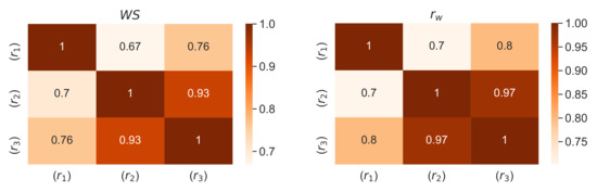
Figure 2.
Comparison of and similarity coefficients [55] for reference rankings –.
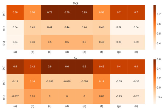
Figure 3.
Comparison of and similarity coefficients [55] between reference rankings – and rankings obtained by using proposed operators (a–h).
From Table 14, we can observe that the best alternative ( or ) mostly maintains the position on top regardless of which technique is used, i.e., TOPSIS, outranking method, TODIM method or the proposed approach. However, a little bit of variation in the ranking order of alternatives is also observed in Table 14. The reason behind these little changes is that, there are some absurd parts of existing operational laws while calculating the multiplications of real numbers of the interval and symbolic translation parameters of linguistic variables of LTS. In any case, in spite of this, we can say that the proposed operators are successful and practical. Furthermore, the current operational laws of linguistic term and the extended linguistic terms at some point result in conflicting outcomes in light of the fact that their operational values surpass the limits of LTSs. Be that as it may, the operational values utilizing the proposed operators for H2TLSs do not surpass the limits during the calculation procedure. Moreover, the computational work is a lot smaller during the time spent conducting estimations by utilizing these operators. Taking everything into account, the attributes of the suggested approach are described as follows:
- Linguistic preference structure along with the symbolic translation are simultaneously utilized in the evaluation procedure of alternatives to make assessments under specific criteria. This can portray the fuzziness and uncertainty of DMs all the more appropriately;
- The proposed H2TLBM, H2TLHM, H2TLGBM and H2TLGHM operators for H2TLSs are exceptionally helpful and successful that can be utilized to aggregate the DMs preferences in MCGDM problems which can exhibit the predominance of the proposed approach.
- The proposed operators are suitable for a linguistic variable with the translational arguments and permits the DMs to have more options while choosing aggregation techniques utilizing H2TLSs.
5. Conclusions
This paper investigates some novel operational laws for H2TLSs to analyze attributes in MCGDM, which carries the values of the alternative as H2TLEs. We presented some hesitant 2-tuple linguistic aggregation operators that are more common and versatile, namely H2TLBM, H2TLHM, H2TLGBM and H2TLGHM operators. We also analyzed specific cases and properties related to the established operators. In addition, we proposed a method for MCGDM based on H2TBM, H2TLHM, H2TLGBM and H2TLGHM operators using H2TLS. Finally, the procedure of the developed technique was illustrated with the help of an example, and the impact of particular parameters p and q is talked about. The essential benefits of our approach over other techniques include its capacity to aggregate the information in the form of H2TLSs and the ability that the linguistic values do not surpass the limits of LTSs during the computation. This can keep away from loss of data and distortion of information that was initially provided by the DMs. Furthermore, we would diversify the suggested operators into many other uncertain circumstances and apply them in risk management, supply chain management and cluster analysis in our future work. The interesting direction can also be a comparison in the field of decision making and medical diagnosis problems and try to combine them with [56].
Author Contributions
Conceptualization, S.F., W.S., N.S., A.u.R. and J.W.; methodology, S.F., W.S., N.S., A.u.R. and J.W.; software, S.F., W.S., N.S., A.u.R. and J.W.; validation, S.F., W.S., N.S., A.u.R. and J.W.; formal analysis, S.F., W.S., N.S., A.u.R. and J.W.; investigation, S.F., W.S., N.S., A.u.R. and J.W.; resources, S.F., W.S., N.S., A.u.R. and J.W.; data curation, S.F., W.S., N.S., A.u.R. and J.W.; writing—original draft preparation, S.F., W.S., N.S. and A.u.R.; writing—review and editing, S.F., W.S., N.S., A.u.R. and J.W.; supervision, S.F., W.S., A.u.R. and J.W.; project administration, W.S.; funding acquisition, J.W. All authors have read and agreed to the published version of the manuscript.
Funding
The work was supported by the project financed within the framework of the program of the Minister of Science and Higher Education under the name “Regional Excellence Initiative” during the period 2019–2022, Project Number 001/RID/2018/19; the amount of financing: PLN 10.684.000,00 (J.W.).
Institutional Review Board Statement
Not applicable.
Informed Consent Statement
Not applicable.
Data Availability Statement
Not applicable.
Acknowledgments
The authors would like to thank the editor and the anonymous reviewers, whose insightful comments and constructive suggestions helped us significantly improve the quality of this paper.
Conflicts of Interest
The authors declare no conflict of interest.
References
- Behzadian, M.; Otaghsara, S.K.; Yazdani, M.; Ignatius, J. A state-of the-art survey of TOPSIS applications. Expert Syst. Appl. 2012, 39, 13051–13069. [Google Scholar] [CrossRef]
- Paradowski, B.; Więckowski, J.; Dobryakova, L. Why TOPSIS does not always give correct results? Procedia Comput. Sci. 2020, 176, 3591–3600. [Google Scholar] [CrossRef]
- Pei, Z.; Liu, J.; Hao, F.; Zhou, B. FLM-TOPSIS: The fuzzy linguistic multiset TOPSIS method and its application in linguistic decision making. Inf. Fusion 2019, 45, 266–281. [Google Scholar] [CrossRef]
- Liao, H.; Xu, Z.; Zeng, X.J. Hesitant fuzzy linguistic VIKOR method and its application in qualitative multiple criteria decision making. IEEE Trans. Fuzzy Syst. 2014, 23, 1343–1355. [Google Scholar] [CrossRef]
- Więckowski, J.; Sałabun, W. How the normalization of the decision matrix influences the results in the VIKOR method? Procedia Comput. Sci. 2020, 176, 2222–2231. [Google Scholar] [CrossRef]
- Shekhovtsov, A.; Sałabun, W. A comparative case study of the VIKOR and TOPSIS rankings similarity. Procedia Comput. Sci. 2020, 176, 3730–3740. [Google Scholar] [CrossRef]
- Zolfani, S.; Yazdani, M.; Pamucar, D.; Zarate, P. A VIKOR and TOPSIS focused reanalysis of the MADM methods based on logarithmic normalization. arXiv 2020, arXiv:2006.08150. [Google Scholar]
- Stojčić, M.; Zavadskas, E.K.; Pamučar, D.; Stević, Ž.; Mardani, A. Application of MCDM methods in sustainability engineering: A literature review 2008–2018. Symmetry 2019, 11, 350. [Google Scholar] [CrossRef] [Green Version]
- Palczewski, K.; Sałabun, W. Influence of various normalization methods in PROMETHEE II: An empirical study on the selection of the airport location. Procedia Comput. Sci. 2019, 159, 2051–2060. [Google Scholar] [CrossRef]
- Sałabun, W.; Wątróbski, J.; Shekhovtsov, A. Are MCDA Methods Benchmarkable? A Comparative Study of TOPSIS, VIKOR, COPRAS, and PROMETHEE II Methods. Symmetry 2020, 12, 1549. [Google Scholar] [CrossRef]
- Shekhovtsov, A.; Rehman, N.; Faizi, S.; Sałabun, W. On the Analytic Hierarchy Process Structure in Group Decision-Making Using Incomplete Fuzzy Information with Applications. Symmetry 2021, 13, 609. [Google Scholar]
- Đalić, I.; Ateljević, J.; Stević, Ž.; Terzić, S. An integrated swot–fuzzy piprecia model for analysis of competitiveness in order to improve logistics performances. Facta Univ. Ser. Mech. Eng. 2020, 18, 439–451. [Google Scholar]
- Vaidya, O.S.; Kumar, S. Analytic hierarchy process: An overview of applications. Eur. J. Oper. Res. 2006, 169, 1–29. [Google Scholar] [CrossRef]
- Becker, J.; Becker, A.; Sałabun, W. Construction and use of the ANP decision model taking into account the experts’ competence. Procedia Comput. Sci. 2017, 112, 2269–2279. [Google Scholar] [CrossRef]
- Saaty, T.L.; Vargas, L.G. The analytic network process. In Decision Making with the Analytic Network Process; Springer: Berlin/Heidelberg, Germany, 2013; pp. 1–40. [Google Scholar]
- Kheybari, S.; Rezaie, F.M.; Farazmand, H. Analytic network process: An overview of applications. Appl. Math. Comput. 2020, 367, 124780. [Google Scholar] [CrossRef]
- Kizielewicz, B.; Więckowski, J.; Shekhovtsov, A.; Ziemba, E.; Wątróbski, J.; Sałabun, W. Input data preprocessing for the MCDM model: COPRAS method case study. In Proceedings of the 27th Americas Conference on Information Systems, AMCIS 2021, Association for Information Systems, Virtual Conference, 9–13 August 2021. [Google Scholar]
- Stefano, N.M.; Casarotto Filho, N.; Vergara, L.G.L.; da Rocha, R.U.G. COPRAS (Complex Proportional Assessment): State of the art research and its applications. IEEE Lat. Am. Trans. 2015, 13, 3899–3906. [Google Scholar] [CrossRef]
- Wan, S.P.; Xu, G.L.; Dong, J.Y. Supplier selection using ANP and ELECTRE II in interval 2-tuple linguistic environment. Inf. Sci. 2017, 385, 19–38. [Google Scholar] [CrossRef]
- Figueira, J.R.; Mousseau, V.; Roy, B. ELECTRE methods. In Multiple Criteria Decision Analysis; Springer: Berlin/Heidelberg, Germany, 2016; pp. 155–185. [Google Scholar]
- Akram, M.; Garg, H.; Zahid, K. Extensions of ELECTRE-I and TOPSIS methods for group decision-making under complex Pythagorean fuzzy environment. Iran. J. Fuzzy Syst. 2020, 17, 147–164. [Google Scholar]
- Kizielewicz, B.; Wątróbski, J.; Sałabun, W. Identification of Relevant Criteria Set in the MCDA Process—Wind Farm Location Case Study. Energies 2020, 13, 6548. [Google Scholar] [CrossRef]
- Kizielewicz, B.; Dobryakova, L. How to choose the optimal single-track vehicle to move in the city? Electric scooters study case. Procedia Comput. Sci. 2020, 176, 2243–2253. [Google Scholar] [CrossRef]
- Kizielewicz, B.; Kołodziejczyk, J. Effects of the selection of characteristic values on the accuracy of results in the COMET method. Procedia Comput. Sci. 2020, 176, 3581–3590. [Google Scholar] [CrossRef]
- Kizielewicz, B.; Shekhovtsov, A.; Sałabun, W. A New Approach to Eliminate Rank Reversal in the MCDA problems. In International Conference on Computational Science; Springer: Berlin/Heidelberg, Germany, 2021. [Google Scholar]
- Więckowski, J.; Kołodziejczyk, J. Swimming progression evaluation by assessment model based on the COMET method. Procedia Comput. Sci. 2020, 176, 3514–3523. [Google Scholar] [CrossRef]
- Kizielewicz, B.; Dobryakova, L. MCDA based approach to sports players’ evaluation under incomplete knowledge. Procedia Comput. Sci. 2020, 176, 3524–3535. [Google Scholar] [CrossRef]
- Tian, Z.P.; Zhang, H.Y.; Wang, J.Q.; Wang, T.L. Green supplier selection using improved TOPSIS and best-worst method under intuitionistic fuzzy environment. Informatica 2018, 29, 773–800. [Google Scholar] [CrossRef] [Green Version]
- Faizi, S.; Sałabun, W.; Nawaz, S.; ur Rehman, A.; Wątróbski, J. Best-Worst method and Hamacher aggregation operations for intuitionistic 2-tuple linguistic sets. Expert Syst. Appl. 2021, 181, 115088. [Google Scholar] [CrossRef]
- Mi, X.; Tang, M.; Liao, H.; Shen, W.; Lev, B. The state-of-the-art survey on integrations and applications of the best worst method in decision making: Why, what, what for and what is next? Omega 2019, 87, 205–225. [Google Scholar] [CrossRef]
- Wątróbski, J.; Jankowski, J.; Ziemba, P.; Karczmarczyk, A.; Zioło, M. Generalised framework for multi-criteria method selection: Rule set database and exemplary decision support system implementation blueprints. Data Brief 2019, 22, 639. [Google Scholar] [CrossRef]
- Zadeh, L.A.; Klir, G.J.; Yuan, B. Fuzzy Sets, Fuzzy Logic, and Fuzzy Systems: Selected Papers; World Scientific: Singapore, 1996; Volume 6. [Google Scholar]
- Torra, V. Hesitant fuzzy sets. Int. J. Intell. Syst. 2010, 25, 529–539. [Google Scholar] [CrossRef]
- Zadeh, L.A. The concept of a linguistic variable and its application to approximate reasoning—I. Inf. Sci. 1975, 8, 199–249. [Google Scholar] [CrossRef]
- Pei, Z.; Ruan, D.; Liu, J.; Xu, Y. Linguistic Values Based Intelligent Information Processing: Theory, Methods, and Applications; Springer: Berlin/Heidelberg, Germany, 2010; Volume 259. [Google Scholar]
- Herrera, F.; Herrera-Viedma, E. Linguistic decision analysis: Steps for solving decision problems under linguistic information. Fuzzy Sets Syst. 2000, 115, 67–82. [Google Scholar] [CrossRef]
- Wang, J.H.; Hao, J. A new version of 2-tuple fuzzy linguistic representation model for computing with words. IEEE Trans. Fuzzy Syst. 2006, 14, 435–445. [Google Scholar] [CrossRef]
- Herrera, F.; Martínez, L. A 2-tuple fuzzy linguistic representation model for computing with words. IEEE Trans. Fuzzy Syst. 2000, 8, 746–752. [Google Scholar]
- Xu, Z. A method based on linguistic aggregation operators for group decision making with linguistic preference relations. Inf. Sci. 2004, 166, 19–30. [Google Scholar] [CrossRef]
- Rodriguez, R.M.; Martinez, L.; Herrera, F. Hesitant fuzzy linguistic term sets for decision making. IEEE Trans. Fuzzy Syst. 2011, 20, 109–119. [Google Scholar] [CrossRef]
- Delgado, M.; Verdegay, J.L.; Vila, M.A. On aggregation operations of linguistic labels. Int. J. Intell. Syst. 1993, 8, 351–370. [Google Scholar] [CrossRef]
- Herrera, F.; Herrera-Viedma, E. A model of consensus in group decision making under linguistic assessments. Fuzzy Sets Syst. 1996, 78, 73–87. [Google Scholar] [CrossRef]
- Degani, R.; Bortolan, G. The problem of linguistic approximation in clinical decision making. Int. J. Approx. Reason. 1988, 2, 143–162. [Google Scholar] [CrossRef] [Green Version]
- Mendel, J.M. Computing with words and its relationships with fuzzistics. Inf. Sci. 2007, 177, 988–1006. [Google Scholar] [CrossRef]
- Herrera, F.; Martinez, L. An approach for combining linguistic and numerical information based on the 2-tuple fuzzy linguistic representation model in decision-making. Int. J. Uncertain. Fuzziness Knowl. Based Syst. 2000, 8, 539–562. [Google Scholar] [CrossRef]
- Wei, C.; Liao, H. A multigranularity linguistic group decision-making method based on hesitant 2-tuple sets. Int. J. Intell. Syst. 2016, 31, 612–634. [Google Scholar] [CrossRef]
- Beg, I.; Rashid, T. Hesitant 2-tuple linguistic information in multiple attributes group decision making. J. Intell. Fuzzy Syst. 2016, 30, 109–116. [Google Scholar] [CrossRef]
- Faizi, S.; Rashid, T.; Zafar, S. An outranking approach for hesitant 2-tuple linguistic sets. Granul. Comput. 2019, 4, 725–737. [Google Scholar] [CrossRef]
- Faizi, S.; Rashid, T.; Zafar, S. TODIM approach based on score function under hesitant 2-tuple linguistic environment. J. Intell. Fuzzy Syst. 2020, 38, 663–673. [Google Scholar] [CrossRef]
- Bonferroni, C. Sulle medie multiple di potenze. Boll. Dell’Unione Mat. Ital. 1950, 5, 267–270. [Google Scholar]
- Wang, L.; Wang, Y.; Liu, X. Prioritized aggregation operators and correlated aggregation operators for hesitant 2-tuple linguistic variables. Symmetry 2018, 10, 39. [Google Scholar] [CrossRef] [Green Version]
- Verma, R.; Sharma, B.D. Hesitant Fuzzy Geometric Heronian Mean Operators and Their Application to Multi-Criteria Decision Making. Sci. Math. Jpn. 2015, 78, 23–39. [Google Scholar]
- Gou, X.; Xu, Z. Novel basic operational laws for linguistic terms, hesitant fuzzy linguistic term sets and probabilistic linguistic term sets. Inf. Sci. 2016, 372, 407–427. [Google Scholar] [CrossRef]
- Faizi, S.; Rashid, T.; Zafar, S. Additive consistency-based approach for group decision making with hesitant 2-tuple linguistic preference relations. J. Intell. Fuzzy Syst. 2018, 35, 4657–4672. [Google Scholar] [CrossRef]
- Sałabun, W.; Urbaniak, K. A new coefficient of rankings similarity in decision-making problems. In International Conference on Computational Science; Springer: Berlin/Heidelberg, Germany, 2020; pp. 632–645. [Google Scholar]
- Mahmood, T.; Ullah, K.; Khan, Q.; Jan, N. An approach toward decision-making and medical diagnosis problems using the concept of spherical fuzzy sets. Neural Comput. Appl. 2019, 31, 7041–7053. [Google Scholar] [CrossRef]
Publisher’s Note: MDPI stays neutral with regard to jurisdictional claims in published maps and institutional affiliations. |
© 2021 by the authors. Licensee MDPI, Basel, Switzerland. This article is an open access article distributed under the terms and conditions of the Creative Commons Attribution (CC BY) license (https://creativecommons.org/licenses/by/4.0/).