Abstract
This work proposes a stochastic process-based inversion to estimate hydrocarbon resistivity based on multifrequency electromagnetic (EM) data. Currently, mesh-based algorithms are used for processing the EM responses which cause high time-consuming and unable to quantify uncertainty. Gaussian process (GP) is utilized as the alternative forward modeling approach to evaluate the EM profiles with uncertainty quantification. For the optimization, gradient descent is used to find the optimum by minimizing its loss function. The prior EM profiles are evaluated using finite element (FE) through computer simulation technology (CST) software. For validation purposes, mean squared deviation and its root between EM profiles evaluated by the GP and FE at the unobserved resistivities are computed. Time taken for the GP and CST to evaluate the EM profiles is compared, and absolute error between the estimate and its simulation input is also computed. All the resulting deviations were significantly small, and the GP took lesser time to evaluate the EM profiles compared to the software. The observational datasets also lied within the 95% confidence interval (CI) where the resistivity inputs were estimated by the proposed inversion. This indicates the stochastic process-based inversion can effectively estimate the hydrocarbon resistivity in the seabed logging.
1. Introduction
Determining high resistive structures, such as hydrocarbon-saturated reservoirs without wells drilling, is of crucial significance in oil and gas industry. In this context, the traditional surveying technique, such as seismic method, has been employed. The method utilizes sound waves to map the geological subsurface, but, according to Reference [1], the seismic results can be uncertain. Therefore, researchers in Reference [2] introduced seabed logging (SBL) to remotely determine the offshore hydrocarbon-saturated reservoirs and become the complementary tool to the seismic method. Marine controlled-source electromagnetic (CSEM) technique (also known as SBL) employs low-frequency electromagnetic (EM) energy sourced by a very powerful electric dipole, towed by a ship, to characterize high resistive structures (e.g., hydrocarbon) beneath the seabed [3]. This frequency-domain technique relies on a fact that hydrocarbon has higher electrical resistivity than its surroundings. Electrical resistivity of the hydrocarbon can approximately reach 30 to 500 Ωm, while the resistivities of its surroundings, such as seawater and sediment, are approximately 0.5 to 2.0 Ωm and 1.0 to 2.0 Ωm, respectively. The property of the electrical resistivity (inversely proportional to conductivity) plays an important role for the hydrocarbon exploration. Main references of the SBL can be found in References [1,2,3,4,5,6,7,8,9,10,11,12].
Besides capable of detecting the hydrocarbon-saturated reservoirs remotely (i.e., without well drilling), the numerical forward modeling methods used for processing the CSEM data are also very powerful and reliable. Practically, the forward modeling is reliant on an assumption that the property of the resistivity is known. Then, a few processes take place in the forward solution, such as simulating the data based on the model, comparing the simulation with the measured data, and updating the model. The surveying CSEM technique usually employs finite element (FE) or finite difference (FD) methods for the data-processing [13]. FE method is preferable due to its ability to support unstructured meshes in order to represent the complex subsurface realistically. Note that these deterministic numerical methods are mesh-based algorithms which involve complicated integrations and linear system. Even though they are reliable, high computational efforts, in terms of cost and time, are needed especially for solving the integrals and the linear equations [14]. In addition, inverse modeling is also very useful, especially to recover the physical property (e.g., resistivity) of hydrocarbon; however, according to researchers in Reference [14], the inversion scheme needs multiple forward solutions, hence high computational time being required to solve the inversion scheme. Here, the corresponding forward modeling should be able to do the simulation rapidly, especially for the repeated use of number of iterations. SBL applications generate large volume of noisy data captured by all receivers located on the seafloor. Researchers in Reference [1] stated that the CSEM data-processing has become a challenging task to geophysicists. Therefore, quantification of uncertainty in processing the CSEM data is very important in the SBL. The use of the differential equation (DE) methods alone in the forward modeling is not capable of providing the quantification of the uncertainty.
To address these problems, we propose a stochastic process-based inversion methodology to estimate the electrical resistivity of hydrocarbon layer based on the multifrequency SBL data. Gaussian process (GP) regression is a stochastic and nonparametric method which is employed as the alternative forward modeling method that is able to provide the uncertainty quantification. According to researchers in Reference [15], this elegant method can perform very well in the nonlinear modeling problems. In the inverse modeling, gradient descent (GD) method is utilized for the optimization purposes. We use mean squared error (MSE) as the objective function (i.e., loss function) of the optimization. GD acts as the minimizer finder by obtaining the optimal electrical resistivity of hydrocarbon of the observational dataset. The novelty of this work can be described in three ways: (i) making full use of the stochastic process as the EM forward modeling by utilizing knowledge from computer simulation to reduce the computational effort involved in the modeling, (ii) integrating the stochastic approach and the indirect search algorithm in one inversion methodology to recover the hydrocarbon resistivity property, and (iii) applying the proposed inversion to find the resistivity of the hydrocarbon in the SBL application based on the multifrequency marine CSEM data with uncertainty justification. This work could be very advantageous to the petroleum industry to reduce the computational efforts involved in the ad hoc CSEM modeling. The literature reviews on the available methods used in processing the CSEM data are discussed in Section 2.
2. Available Methods Used in Processing CSEM Data
For decades, controlled-source electromagnetic (CSEM) technology has been widely employed in many land-based geophysical explorations [13]. Rising in oil and gas demand has triggered a commercial interest to apply the CSEM technique in ocean-based subsurface exploration [16]. The subsurface could be very complex due to a lateral variation of the subsurface conductivity beneath the seafloor (i.e., sea-bottom sediments). In the electromagnetic (EM) modeling, Maxwell’s equations are solved in a discretized form to compute the propagation of the EM fields. In a 3-D scenario, the subsurface can be discretized using either regular brick, hexahedral, or tetrahedron elements.
According to Reference [13], the electric and magnetic fields within each element can be approximated by either linear or higher order polynomial functions. Researchers in Reference [17] used 3-D finite element (FE) method to compute the EM responses from the reservoir that consists of a set of resistive hydrocarbons separated by conductors in homogeneous and inhomogeneous environments. The resulting computational experiments showed that the presence of the resistive gaps gave a significant impact on the EM fields recorded by the receivers. Researchers in Reference [13] employed linear edge-based FE method for modeling the 3-D CSEM data in anisotropic conductive medium. Besides that, researchers in Reference [18] introduced a new method for processing CSEM data based on redatuming the observational data from the actual receivers into the virtual receivers. To compute the EM fields in the virtual receivers, Stratton-Chu type integral transformation was used in the research study. Next, 2.5-D FE method was used by researchers in Reference [19] as its forward modeling code for marine CSEM application in Niger Delta. Adaptive FE method has been known as a robust numerical modeling approach in complex environment. It adaptively refines the FE mesh using error estimator of a priori to produce high quality of EM responses for all the refinements though it caused high computational time. Researchers in Reference [20] used FE, namely linear edge FE method, for their computational implementation of the CSEM application. Other than that, parallel edge-based tool for geophysical EM modeling (PETGEM) was used by researchers in Reference [21] for 3-D CSEM forward modeling by employing Nédélec edge finite element method (EFEM). The EFEM can support the unstructured tetrahedral meshes and offers a good compromise between its accuracy and the number of degrees of freedom. To our knowledge, most of the existing numerical EM modeling techniques are mesh-based algorithms. These differential equation (DE) methods involve very large computational domain to satisfy to the corresponding boundary condition in the modeling. Other than the DE methods, some literature also reported the use of integral equation (IE) method for the EM modeling. However, according to researchers in Reference [22], the matrix system involved in the IE method needs significantly high computational effort in terms of time and memory.
3. Background of the Proposed Methodology
The proposed inversion methodology consists of two frameworks, which are Gaussian process (GP) as the forward modeling method, and gradient descent (GD) used for the optimization involved in the inversion scheme.
3.1. Stochastic Process–Gaussian Process
Gaussian process (GP) is a random function which consists of a collection of random variables that are treated as Normal (i.e., gaussian) distribution [23,24]. A model of GP is defined by a vector of its mean function, , and a matrix composed by its covariance function, . The distribution can be expressed as . GP is a probabilistic and nonparametric method which capable of fitting functional forms reliant on the domain observations. According to Reference [25], this stochastic approach has a property that differs from most of the other black-box identification approaches. It searches for the correlations among the known knowledge rather than approximating the model by trying to fit the basis function parameters. GP can provide the predictive mean (i.e., most likely output) and predictive variance (i.e., confidence interval (CI)) through the Bayesian inference. It places a prior on the function space without parameterizing the function and then generates posterior distribution over the function. Researchers in Reference [26] stated that a GP model can be utilized as a surrogate model for intricate mathematical model that needs high computational time to solve.
GP has been used in many applications due to its flexibility, such as in the engineering fields, geo-statistics, electronics, machine learning, etc. Researchers in Reference [27] mentioned that the GP is capable of decreasing the complexity of the computer vision with a finer performance of reconstructions. In addition, researchers in Reference [28] compared the performance of an improved GP model with other methods, such as multiple linear regression (MLR) and artificial neural network (ANN), in predicting roadway broken road zone. The results showed that the hybrid model gave the best performance in terms of coefficient of determination (), root mean squared error (RMSE), and variance accounted for (VAF). In geophysics field, researchers in Reference [29] stated that GP can provide reliable porosity and permeability information to the well analysis. Besides that, GP was also fully utilized by researchers in Reference [30] in the seismic signal detection. The study inferred that the GP was able to produce higher rate of detection and lower rate of false alarm, especially for the weak seismic signals. Next, researchers in Reference [31] proposed an improved methodology for active learning in the GP regression to predict the black-box functions. The proposed method revealed better RMSE with a fewer number of points compared to the other famous methods. Researchers in Reference [32] also enhanced the GP regression for estimating the state-of-health (SOH), and the results showed that the proposed method was capable of reducing the computational complexity with better estimation accuracy.
3.2. Gradient Descent
Gradient descent (GD) is a famous iterative method used for updating parameters of a function. GD updates the model by minimizing its objective function based on a first derivative (i.e., slope) property. Determining the slope can inform the direction of the model parameters (whether to decrease or increase), and it also could tell the step size that should be taken by the model to reach the optimum point. GD is also known as steepest descent method, where it optimizes the objective function by moving in negative direction of the slope iteratively. In the GD method, the step size is called as learning rate, . A smaller can learn the function area precisely since the slope is frequently recalculated. But, if the is not carefully parameterized, the optimization may require high processing time to converge and reach the optimum point. Meanwhile, a bigger can extend over larger area of the function but overshooting the optimum point may occur. Thus, sensible parameterization of the step size implies the efficiency of the GD optimization.
GD is a well-known method that is commonly used in optimization problems, such as in the applications of machine learning. Researchers in Reference [33] exercised the GD for the purpose of optimizing the vector centers of the consequent layer functions and receptive field matrices in a neuro-fuzzy model. This study relied on the mean squared error (MSE) criterion as its standard of the optimization. Besides that, researchers in Reference [34] employed the GD method to establish nodes operation model for classifying heart conditions based on a deep learning network. Next, researchers in Reference [35] also used GD method to identify the aperture shape in the direct aperture optimization (DAO). Furthermore, this optimization method was also utilized by researchers in Reference [36] to solve the predicting student performance (PSP) by minimizing the error equation, which is its loss function. The study updated the matrices of and in the optimization scheme. In addition, researchers in Reference [37] employed GD to find the optimal parameters of impedance control in an iterative learning control algorithm for the force/position hybrid control to control the trajectory of the hexa-robot. The results revealed that the proposed approach can successfully control the robot as expected. Researchers in Reference [38] also used GD to obtain phase-only computer-generated holograms (CGHs). The study concluded that the GD method needed low time to optimize the distribution of the phase-only CGHs and obtained higher precision images compared to the results obtained when using the Gerchberg-Saxton (GS) algorithm.
4. Methodology
In Section 4, five subsections are discussed, which are, Section 4.1. Developing synthetic seabed logging (SBL) model, Section 4.2. Preprocessing computer simulation outputs, Section 4.3. Developing two-dimensional (2-D) Gaussian process (GP) models, Section 4.4. Electrical resistivity estimation, and Section 4.5. Validation of estimate and GP model.
4.1. Developing Synthetic Seabed Logging Model
A synthetic seabed logging (SBL) application is replicated using the computer simulation technology (CST) software. According to Reference [39], CST Studio Suite® exclusively employs finite element (FE) method as the solver of the electromagnetic (EM) simulation in the low-frequency applications. The synthetic model has the same input parameters, except for the conductivity (inversely proportional to the resistivity) of the hydrocarbon layer and the frequency of the EM signal. The SBL model is replicated with three different background layers, such as air, seawater, and sediment, with an isotropic hydrocarbon layer inside, as depicted in Figure 1.
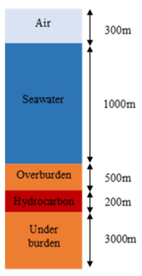
Figure 1.
Representation of the synthetic seabed logging (SBL) model in the computer simulation technology (CST) software. The total height, width, and length are 5000 m, 20,000 m, and 20,000 m, respectively.
Based on Figure 1, sediment layer located above the target layer (i.e., hydrocarbon) is called as overburden, whereas sediment below the target layer is called as under burden. The thickness of overburden (i.e., depth of hydrocarbon) is fixed at 500 m from the seafloor. To make it simpler, all the input parameters of the simulation are summarized in Table 1. Based on Table 1, five different transmission frequencies (i.e., multifrequency) and five resistivities of isotropic target (e.g., 90, 180, 270, 360, and 450 Ωm) are simulated in the SBL modeling. It means that for every frequency, five different EM profiles are generated and these profiles act as the training CST datasets for the data-processing purposes. Note that the set-up is fixed for the case of static source-receiver separation distances. The source (i.e., transmitter) is placed in the seawater at the center of the model with coordinate of (height = 1270 m, width = 10,000 m, length = 10,000 m), and the inline receivers are located along the seafloor. Hence, all the generated CST datasets are symmetrical from the model center to the right and left boundaries.

Table 1.
Input parameters of the computer simulation.
4.2. Preprocessing Computer Simulation Outputs
As discussed in Reference [40], the SBL data interpretation is based on an assumption that the existence of target bodies can be preidentified by normalizing the magnitude versus offset (MVO) between the target responses (with hydrocarbon) and the reference responses (without hydrocarbon). The normalized MVO can be calculated by dividing the target responses with the reference responses. The existence of the potential target bodies can be detected if the ratio of normalization is greater than 1.0.
The same input parameters are used for replicating the reference model, as indicated in Table 1 and presented in Section 4.1, but the hydrocarbon information is not included. After generating the multifrequency reference model and preprocessing the electromagnetic (EM) profiles by considering the normalized MVO and symmetricity of the model, only 93 datapoints per dataset are used for the GP modeling (discussed in the next subsection), which are taken from source-receiver separation distances of 10,845.77–20,000 m.
4.3. Developing Two-Dimensional Gaussian Process Models
Gaussian process machine learning (GPML) MATLAB codes are used for the Gaussian process (GP) regression. The GPML codes can be found in Reference [41]. As mentioned earlier, the GP regression is employed to evaluate the EM profiles at various unobserved resistivities of hydrocarbon. For every frequency, all five CST datasets, as expressed in Equation (1), are treated as the GP training datasets.
where = 93. The -dimensional input vector and its corresponding output vector can be simply written as and , respectively. indicates -by- matrix (i.e., ), and indicates -by- column vector (i.e., ). In this work, the input is bivariate, , where stands for the source-receiver separation distance (i.e., offset), and is the electrical resistivity of the hydrocarbon layer, whereas the corresponding output is the magnitude of electric field (E-field).
To evaluate the EM profiles at unobserved resistivity inputs conforming to the testing input , the posterior distribution is defined as in Equation (2):
where and are the predictive mean and variance, respectively. These two terms are defined in Equations (3) and (4). Since the resistivity of hydrocarbon is the only parameter that is varied, thus (i.e., remains unchanged). One hundred and sixteen unobserved target resistivities, which are 93–447 Ωm with an increment of 3 Ωm each (excluding the training input points), are set as the desired information. Therefore, for every frequency, there are entirely 121 EM profiles (including the training datasets) evaluated in the GP model.
and
where
Based on Equations (3)–(5), is an -by- covariance matrix amongst the , is an -dimensional noise covariance matrix, is an -by- covariance matrix between the and , and is a covariance matrix of . Note that, in the context of this work, all these covariance matrices are composed of the squared exponential (SE) covariance function, where Equation (6) is utilized to compute every element of the matrices.
where hyperparameters . and represent the isotropic length scale and the signal variance, respectively. Note that the SE covariance function is used to govern the GP realizations smoothness which is dictated by the computer simulation outputs. According to Reference [42], GP regression with the SE covariance function is infinitely differentiable. This is an advantageous for any inversion scheme that relies on the derivative basis such as the gradient descent (GD) method.
Here, Equations (2)–(6) need the computation of the hyperparameters . In the GP regression, this is computed by minimization of the negative log marginal likelihood (NLML) using the gradient-based approach. The equation of NLML is expressed in Equation (7):
Researchers in Reference [29] mentioned that the logarithmic identifier used in Equation (7) is to simplify the expression of integrals involved in the marginal likelihood method. Once the is successfully computed, the GP predictive distribution is defined by using Equations (3) and (4). Here, the is the best estimate of (i.e., predictive mean) which represents the magnitude of E-field at the , and the represents the predictive variance of the in terms of 95% confidence interval (CI) (±two standard deviations). This feature expresses the reliability of the .
4.4. Electrical Resistivity Estimation
It must be noted here that the developed GP model is denoted as where all the EM profiles are evaluated at all training and testing input parameters. For every frequency, consists of 121 EM profiles observed at 93 points of offset from 10,845.77 m to 20,000 m with 121 different resistivities of hydrocarbon (90–450 Ωm, with a gap of 3 Ωm). Assume that the observational dataset is observed at = 93 points of offset, and there is a potential target layer resides 500 m underneath the seafloor with “unknown” resistivity. Then, the least square criterion is formed between the and the in order to determine the target electrical resistivity of the . This work uses mean squared error (MSE) as the objective function of the optimization scheme. Generally, MSE calculates the mean amount of squared differences between the and . The objective function is defined in Equation (8).
where = 121. The objective function is a function of . Thus, Equation (8) is minimized over the , and the minimizer indicates the estimate of the target resistivity. For every frequency, all the computed are then plotted in order to observe the trend of the function. From the trend, a random initial guess of target resistivity can be specified. Since this is a minimization procedure, the decreasing trend of the function is the key idea of choosing the suitable initial guess. To make the process runs efficiently, a point closes to the minimum zero-gradient point is selected as the initial guess, and the iteration index is set to zero. Here, the initial minimizer is denoted as .
After specifying the initial guess, the first-partial derivative of the is defined with respect to , as derived in Equation (9).
where is the first derivative of the GP model with respect to . As mentioned before, the GP model is composed by the predictive mean , shown in Equation (3). Thus, the derivative of the with respect to the is written in Equation (10).
where is the derivative of the covariance matrix between and with respect to the (specifically with respect to ). In order to find the , the derivative of the SE covariance function with respect to is derived. The equation is shown in Equation (11):
The next step is finding the update of the . Based on the GD method, the update can be computed by using Equation (12).
where is the learning rate. To gain more knowledge about the learning rate, in the context of this work, positive values of 10, 1, 0.1, 0.01, 0.001, and 0.0001 are used as the indicator of which range of can give the significant optimization. For the update, the changes between the subsequent update (i.e., minimizer) and the total number of iterations are set to be at most 0.05% and 100, respectively. Equation (13) is used to calculate the subsequent changes of each updated minimizer:
For every iteration, GP regression is utilized to evaluate the EM profile at every update. The new objective function between the and is computed using Equation (14):
Besides identifying the subsequent changes of the update and the number of iterations, the new objective function for every iteration also needs to be verified. One criterion is added as the threshold where the objective function must always converge. In other words, must be always smaller than . Each iteration must satisfy these stopping criteria to continue the optimization process. The flow is repeated until the stopping criteria (i.e., threshold) are neglected, then the iteration stops, and the optimal hydrocarbon resistivity for the is concluded. The methodological flow of the proposed inversion is depicted in Figure 2.
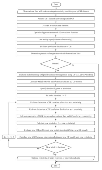
Figure 2.
Methodological flow of the proposed methodology. In the context of this work, all the simulation models are models with presence of the hydrocarbon. Thus, the step of determining the target layer is not discussed in this work. w.r.t. indicates with respect to.
4.5. Validation of Estimate and Gaussian Process Model
To determine the reliability of the estimates of hydrocarbon resistivity obtained by the inversion methodology, this work calculates the absolute error between the estimate and the computer simulation input. The equation of the absolute error is shown in Equation (15).
where indicates the simulation input, and is the target resistivity estimated by the stochastic process-based inversion. Furthermore, the Gaussian process (GP) model is also validated by calculating the mean squared deviation (MSD), and root mean squared deviation (RMSD) between the electromagnetic (EM) profile evaluated by the GP model and EM response modeled by the finite element (FE) method through the computer simulation technology (CST) software at the unobserved input points. Note that the EM responses modeled by the FE are assumed as the true EM values. The equations of the MSD and RMSD are formulated in Equations (16) and (17), respectively.
and
where and represent the EM response modeled by the FE and GP methods, respectively.
5. Algorithms of the Proposed Methodology
Algorithm 1 shows the steps involved in the forward Gaussian process (GP) modeling, whereas the process of the inversion scheme for each frequency developed in this work is shown in Algorithm 2.
| Algorithm 1 Forward Gaussian Process (GP) Modeling |
| Input: Training input: Source-receiver separation distances (i.e., offsets) and hydrocarbon resistivities Training output: Magnitude of electric field (E-field) |
| Steps: |
| 1. Optimize the hyperparameters 2. Define the testing inputs (i.e., unobserved hydrocarbon resistivities) 3. Compute the covariance matrices 4. Evaluate the GP predictive distribution (i.e., predictive mean and variance) |
| Output: Two-dimensional (2-D) GP model which consists of various electromagnetic (EM) profiles (i.e., magnitude of electric field) at the unobserved hydrocarbon resistivities |
| Algorithm 2 Stochastic process-based Inversion |
| Input: Two-dimensional (2-D) GP models at various hydrocarbon resistivities (observed and unobserved) Observational dataset with “unknown’ resistivity of isotropic hydrocarbon |
| Steps: |
|
| Output: The optimal electrical resistivity of hydrocarbon of the observational dataset |
6. Results and Discussion
It must be noted here that all the training datasets were evaluated using the finite element (FE) method, which was exclusively employed by the computer simulation technology (CST) software to solve the low-frequency problems. All the multifrequency computer simulation datasets are depicted in Figure 3.

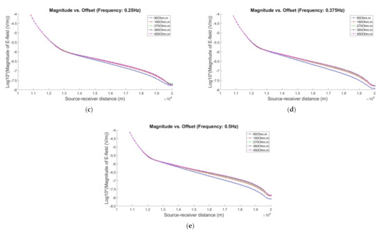
Figure 3.
Magnitude of electric field (E-field) versus offset for five different hydrocarbon resistivities (90, 180, 270, 360, and 450 Ωm) for five different transmission frequencies: (a) 0.0625 Hz, (b) 0.125 Hz, (c) 0.25 Hz, (d) 0.375 Hz, and (e) 0.5 Hz.
Based on Figure 3, the x- and y-axes indicate the source-receiver separation distance and magnitude of E-field in logarithmic scale, respectively. In this work, we observed 93 points of offset, which were from 10,845.77 m to 20,000 m. In addition, we tested multiple transmission frequencies to identify which frequency can give the best estimation of the hydrocarbon electrical resistivity based on the proposed inversion methodology given specific model conditions. To make the figure interpretable, the zoom-in scaled version of Figure 3 at far source-receiver separation distances is provided and depicted in Figure 4.

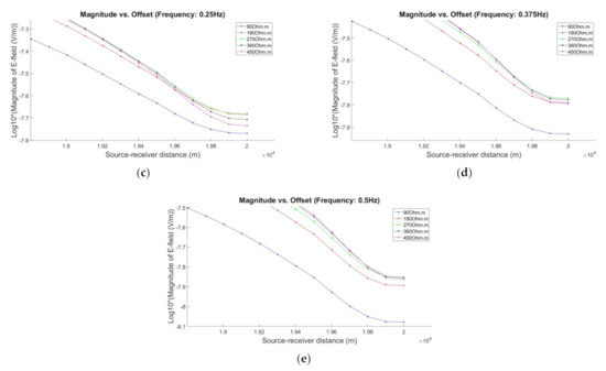
Figure 4.
The zoom-in scaled of magnitude of electric field (E-field) versus offset at far source-receiver separation distances for five different transmission frequencies: (a) 0.0625 Hz, (b) 0.125 Hz, (c) 0.25 Hz, (d) 0.375 Hz, and (e) 0.5 Hz.
From Figure 4, we can see that, when using higher frequency (i.e., 0.5 Hz), the electromagnetic (EM) signals attenuate rapidly along the lower electrical resistivity of hydrocarbon (i.e., 90 Ωm). Lower frequency gave better resolution of magnitude of E-field at far offset distances especially when the hydrocarbon resistivities were higher than 90 Ωm. This is because low-frequency of EM signals less attenuate along the high-resistive medium. We believed that the property of multiple frequencies of EM signal in the seabed logging could give unique clarification to each estimation made by the stochastic process-based inversion methodology.
We utilized all the computer simulation datasets to be used as the training datapoints in the Gaussian process (GP) modeling. For every frequency, we developed a two-dimensional (2-D) GP model which consisted of EM profiles at all training and testing hydrocarbon resistivities. All the contour plots of the 2-D GP model are shown in Figure 5. Based on Figure 5, the x- and y-axes indicate the 93 points of offset and 121 target resistivities, respectively. The log 10 of magnitude of E-field is represented in the color codes. We developed these multifrequency 2-D GP models to evaluate as many EM profiles as possible by fully utilizing the computer simulation datasets. This information is very useful for the inversion scheme. Note that generating all the multifrequency 121 EM profiles using the CST software could consume high computational time, which is approximately 10 h. Meanwhile, the GP modeling only need around 25 min for the prior data acquisition using the computer simulation and approximately less than 1 min to develop all the 2-D GP models at the unobserved inputs. This proves that, in the context of this study, the forward GP modeling can provide more “untried” information with lower computational time compared to the time taken by the mesh-based modeling.
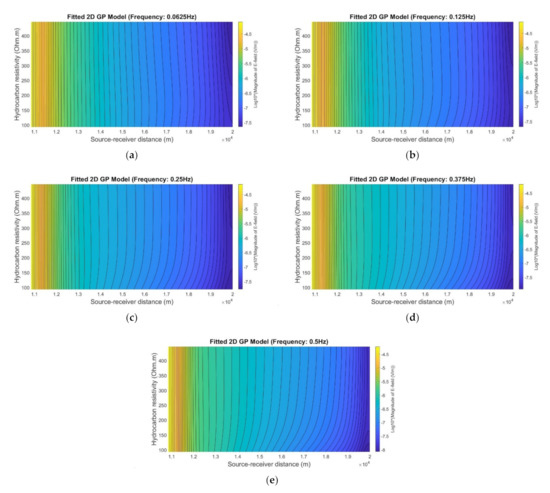
Figure 5.
Two-dimensional (2-D) Gaussian process (GP) model with 121 different electromagnetic (EM) profiles for multiple transmission frequencies; (a) 0.0625 Hz, (b) 0.125 Hz, (c) 0.25 Hz, (d) 0.375 Hz, and (e) 0.5 Hz.
In order to validate the reliability of each of the 2-D GP models, we calculated the mean squared deviation (MSD) and root mean squared deviation (RMSD) between the GP models and the EM responses modeled by the finite element (FE) at eight random unobserved hydrocarbon resistivities chosen in this research work which were 120 Ωm, 150 Ωm, 210 Ωm, 240 Ωm, 300 Ωm, 330 Ωm, 390 Ωm, and 420 Ωm. The resulting MSDs and RMSDs for frequencies of 0.0625, 0.125, 0.25, 0.375, and 0.5 Hz are tabulated in Table 2 and Table 3, respectively.

Table 2.
Mean squared deviation (MSD) results.

Table 3.
Root mean squared deviation (RMSD) results.
Based on Table 2 and Table 3, we can see that all the MSD and RMSD values for every frequency are very small. It shows that the EM profiles evaluated by the GP regression are significantly close to its true values (i.e., EM responses modeled by the FE method). This implies that the GP regression is capable of evaluating multifrequency EM profiles at various unobserved input parameters accurately with low time consumption.
In the context of this work, we generated three different multifrequency observation datasets separately using the CST software which the resistivities of the hydrocarbon were assumed to be “unknown”, i.e., 100 Ωm, 200 Ωm, and 400 Ωm. To avoid biased, we purposely selected these “unknown” hydrocarbon resistivities since there was no information of the resistivities in the developed forward GP model. As mentioned before, the goal of this work was to find the best estimate of hydrocarbon resistivity of the observational dataset by minimizing the mean squared error (MSE). A small MSE indicates that the GP model gives the most likely EM responses for the observational dataset, thereby presenting the best information of the hydrocarbon resistivity. Here, we provide plots of MSE versus hydrocarbon resistivity for every frequency in Figure 6 (for 100 Ωm), Figure 7 (200 Ωm), and Figure 8 (400 Ωm).

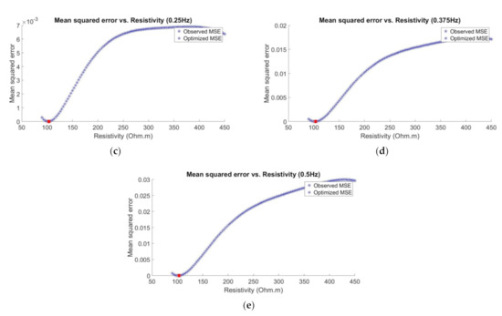
Figure 6.
Mean squared error (MSE) versus hydrocarbon resistivity for multiple transmission frequencies (Observational dataset 1 with “unknown” resistivity of 100 Ωm): (a) 0.0625 Hz, (b) 0.125 Hz, (c) 0.25 Hz, (d) 0.375 Hz, and (e) 0.5 Hz.
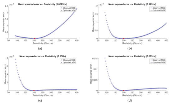
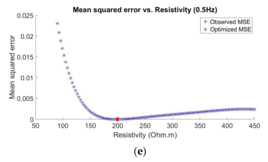
Figure 7.
Mean squared error (MSE) versus hydrocarbon resistivity for multiple transmission frequencies (Observational dataset 2 with “unknown” resistivity of 200 Ωm): (a) 0.0625 Hz, (b) 0.125 Hz, (c) 0.25 Hz, (d) 0.375 Hz, and (e) 0.5 Hz.
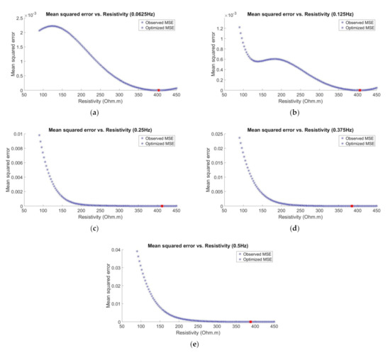
Figure 8.
Mean squared error (MSE) versus hydrocarbon resistivity for multiple transmission frequencies (Observational dataset 3 with “unknown” resistivity of 400 Ωm): (a) 0.0625 Hz, (b) 0.125 Hz, (c) 0.25 Hz, (d) 0.375 Hz, and (e) 0.5 Hz.
By referring to Figure 6, Figure 7 and Figure 8, the x- and y-axes indicate the hydrocarbon resistivities involved in the 2-D GP model and the computed MSE values, respectively. The blue points are the 121 MSEs at the respective hydrocarbon resistivities, whereas the red points represent the optimized MSEs with respect to the updated minimizers. We also monitored the status of the convergence for every optimization. Thus, Figure 9, Figure 10 and Figure 11 show the plots of MSE versus number of iterations for every observational dataset and transmission frequency.
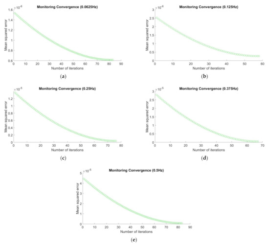
Figure 9.
Mean squared error (MSE) versus number of iterations for multiple transmission frequencies (Observational dataset 1 with “unknown” resistivity of 100 Ωm): (a) 0.0625 Hz, (b) 0.125 Hz, (c) 0.25 Hz, (d) 0.375 Hz, and (e) 0.5 Hz.
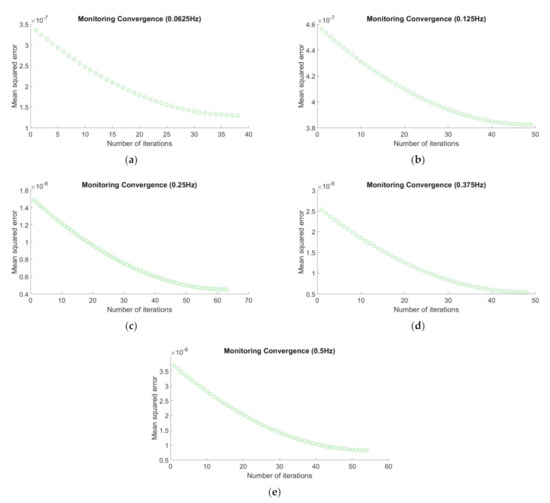
Figure 10.
Mean squared error (MSE) versus number of iterations for multiple transmission frequencies (Observational dataset 2 with “unknown” resistivity of 200 Ωm): (a) 0.0625 Hz, (b) 0.125 Hz, (c) 0.25 Hz, (d) 0.375 Hz, and (e) 0.5 Hz.

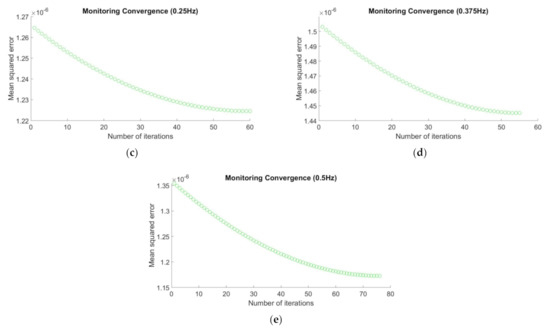
Figure 11.
Mean squared error (MSE) versus number of iterations for multiple transmission frequencies (Observational dataset 3 with “unknown” resistivity of 400 Ωm): (a) 0.0625 Hz, (b) 0.125 Hz, (c) 0.25 Hz, (d) 0.375 Hz, and (e) 0.5 Hz.
In Figure 9, Figure 10 and Figure 11, the x- and y-axes indicate the number of iterations and the computed MSEs, respectively. Based on these figures, we can see that all the optimizations converged to the smallest MSE with less than 100 iterations (maximum iterations number). Here, the most important thing is all the optimizations converged and stopped at the smallest MSE values and approaching to zero. It agrees the main goal of optimization scheme which is to minimize the loss function. Next, in order to make all the figures obtained easier to interpret, we tabulate all the resulting estimates, the validation results (i.e., absolute error), and the learning rate used for every observational data and frequency in table below.
Based on Table 4, all the number of iterations were less than 100 (i.e., the maximum number of iterations). Different learning rate was used for every frequency of the observational dataset. From the table, we can see all the computed MSE were very small. Moreover, for the frequency of 0.0625 Hz, only 72.289 s, 35.775 s, and 33.923 s were taken by the stochastic process-based inversion to estimate 104.03 Ωm, 201.45 Ωm, and 402.22 Ωm, respectively, whereas, for the frequency of 0.125 Hz, the inversion took 50.482 s, 44.682 s, and 46.848 s to estimate 102.72 Ωm, 198.08 Ωm, and 404.34 Ωm, respectively. For the frequency of 0.25 Hz, 63.797 s, 55.898 s, and 51.133 s were needed to estimate 102.17 Ωm, 197.51 Ωm, and 410.64 Ωm, respectively. Next, for the frequency of 0.375 Hz, the time taken by the proposed methodology to yield 102.01 Ωm, 197.93 Ωm, and 383.43 Ωm were 57.818 s, 42.565 s, and 49.087 s, respectively. The last one, for the frequency of 0.5 Hz, only 68.353 s, 47.105 s and 65.238 s was needed by the inversion methodology to produce estimates of 101.91 Ωm, 198.20 Ωm, and 386.18 Ωm, respectively. On average, the GP-inversion only took 52.333 s to obtain the optimal hydrocarbon resistivity. This indicates that the proposed inversion methodology could solve the forward and inverse modeling rapidly. In addition, to observe the trend of the hydrocarbon resistivity estimations based on the multifrequency property, we plotted the calculated absolute errors versus the true resistivity for every tested transmission frequency. The plot is depicted in Figure 12.

Table 4.
The main stochastic process-based inversion results.
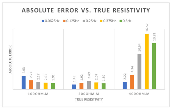
Figure 12.
Absolute error versus true resistivities of 100 Ωm, 200 Ωm, and 400 Ωm for multifrequency property.
From Figure 12, the x- and y-axes indicate the true resistivity and absolute error, respectively. Based on this figure, we can infer that the frequency of 0.5 Hz gave better hydrocarbon resistivity estimation for the observational dataset 1 (true resistivity = 100 Ωm) with the absolute error of 1.91 compared to the other absolute errors when using 0.0625 Hz, 0.125 Hz, 0.25 Hz, and 0.5 Hz. But, when the true resistivity increased, the frequency of 0.0625 Hz gave smaller absolute errors, which were 1.45 for the observational dataset 2 (true resistivity = 200 Ωm) and 2.22 for the dataset 3 (true resistivity = 400 Ωm) compared to the other absolute errors. This is because, in the seabed logging (SBL) applications, lower transmission frequency is used to get far propagation of the EM signals. This feature is normally employed when the location of the target bodies is deep from the seafloor. Besides that, lower frequency also attenuates slowly along the high-resistive bodies, such as hydrocarbon. Thus, far propagation of the EM signals beneath the seabed can be achieved when the embedded bodies have high electrical resistivity. Since the depth of hydrocarbon layer set in this work was fixed at 500 m from the seafloor, the frequency of 0.5 Hz gave the best resistivity estimation when the resistivity of the hydrocarbon layer was 100 Ωm. Meanwhile, when the hydrocarbon resistivity is 200 Ωm and above, the frequency of 0.0625 Hz gave the best estimation of the hydrocarbon resistivity.
Based on those results, its uncertainty quantifications produced by the GP modeling also were investigated. In the context of this work, the uncertainty quantifications for estimates of 101.91 Ωm (at frequency of 0.5 Hz), 201.45 Ωm (at frequency of 0.0625 Hz), and 402.22 Ωm (at frequency of 0.0625 Hz) were examined. EM profiles for these three estimates were evaluated by the GP regression separately, and the predictive variances for each profile were computed in order to determine whether the observational datasets lie within the 95% confidence interval (CI) of the respective GP model or not. If the observational datasets (with 100, 200, and 400 Ωm) fail to fit in the CI of the respective forward GP model, it means that the proposed methodology is unable to provide reliable resistivity information. For the estimate of 101.91 Ωm, only 1.08% of the EM responses over 93 datapoints per EM profile lied outside the 95% CI. Meanwhile, for the other two estimates, only 4.30% of the EM responses lied outside its respective CI for both estimates. By following the testing of significance for hypothesis testing, all the percentages were less than the 5% level of significance. Thus, it can be inferred that the observational datasets significantly lied within the 95% CI of the GP models where its hydrocarbon resistivity inputs were estimated by the stochastic process-based inversion.
7. Conclusions
We proposed stochastic process-based inversion to estimate the electrical resistivity of isotropic hydrocarbon layer based on multifrequency synthetic seabed logging (SBL) model. Five different transmission frequencies were tested which were 0.0625, 0.125, 0.25, 0.375, and 0.5 Hz to determine the effect of the multifrequency property of the SBL application in estimating the hydrocarbon resistivity by using the proposed inversion methodology. We employed the stochastic process, namely Gaussian process (GP) regression, as the alternative forward modeling method to evaluate the electromagnetic (EM) profiles at various unobserved resistivities with uncertainty quantification by utilizing the prior knowledge generated through the computer simulation technology (CST) software. Based on the calculated deviations (presented in Table 2 and Table 3), we proved that the GP was well-fitted to evaluate the EM profiles even at the unobserved resistivity inputs. In addition to that, GP also took significantly lower computational time (approximately 26 min including the prior data acquisition) to evaluate the 121 EM profiles compared to the time that could be taken by the software (approximately 10 h).
Next, for the inversion scheme, we proved that the proposed methodology can efficiently estimate the electrical resistivity of the hydrocarbon layer with low time consumption, with the average time of 52.333 s. The objective function also converged, and the optimization stopped at the smallest mean squared error (MSE). The computed absolute errors also agreed the nature or behavior of multifrequency EM data. For the case of the observational dataset 1, the stochastic process-based inversion was significantly capable of estimating the hydrocarbon resistivity when the transmission frequency used was 0.05 Hz, while, for the case of the observational datasets 2 and 3, frequency of 0.0625 Hz gave better hydrocarbon resistivity estimation. This is because lower frequency of EM signal attenuates slower along the medium with higher resistivity. The choice of the transmission frequency practiced in the SBL applications can be predetermined based on the prior knowledge of the hydrocarbon resistivity. In addition, we also fully utilized the uncertainty quantification feature (i.e., predictive variance) provided by the GP. By following the testing of significance for hypothesis testing, all the percentages of the observational datapoints outside the 95% confidence interval (CI) of the respective GP model were less than 5% level of significance. This showed the observational datasets significantly lied within the uncertainty quantification computed by the GP where the resistivity inputs were estimated by the inversion methodology. Therefore, the stochastic process-based inversion methodology can be fully utilized to effectively estimate the hydrocarbon resistivity in the SBL applications with low computational efforts. This attempt is very useful for the EM data-processing, especially to recover the electrical resistivity distribution of the hydrocarbon reservoir. Consequently, this attempt could de-risk the offshore hydrocarbon exploration.
Author Contributions
Conceptualization, H.D. and S.C.D.; methodology, S.C.D. and M.N.M.A.; software, H.D.; validation, S.C.D., K.A.M.N., and M.N.M.A.; writing—original draft preparation, M.N.M.A.; writing—review and editing, H.D., K.A.M.N., and M.N.M.A.; supervision, H.D., K.A.M.N., and S.C.D.; funding acquisition, H.D. and S.C.D. All authors have read and agreed to the published version of the manuscript.
Funding
This work was supported by Yayasan Universiti Teknologi PETRONAS–Fundamental Research Grant (YUTP–FRG) with cost center of 015LC0-055.
Institutional Review Board Statement
Not applicable.
Informed Consent Statement
Not applicable.
Data Availability Statement
The data presented are openly available in Mendeley Data at doi:10.17632/kvtxc2w4sj.1. The data can be found here http://dx.doi.org/10.17632/kvtxc2w4sj.1.
Acknowledgments
The authors are grateful to Universiti Teknologi PETRONAS (UTP) for the facilities provided.
Conflicts of Interest
The authors declare no conflict of interest.
References
- Ellingsrud, S.; Eidesmo, T.; Sinha, M.C.; MacGregor, L.M.; Constable, S.C. Remote sensing of hydrocarbon layers by sea bed logging (SBL): Results from a cruise offshore Angola. Lead. Edge 2002, 20, 972–982. [Google Scholar] [CrossRef]
- Eidesmo, T.; Ellingsrud, S.; MacGregor, L.M.; Constable, S.; Sinha, M.C.; Johansen, S.; Kong, F.N.; Westerdahl, H. Sea bed logging (SBL), a new method for remote and direct identification of hydrocarbon filled layers in deep water areas. First Break 2002, 20, 144–152. [Google Scholar]
- Edwards, N. Marine controlled-source electromagnetics: Principles, methodologies, future commercial applications. Surv. Geophys. 2005, 26, 675–700. [Google Scholar] [CrossRef]
- Hesthammer, J.; Boulaenko, M. The offshore EM challenges. First Break 2005, 23, 59–66. [Google Scholar] [CrossRef]
- Carazzone, J.J.; Burtz, O.M.; Green, K.E.; Pavlov, D.A.; Xia, C. Three dimensional imaging of marine controlled source EM data. SEG Tech. Program Expand. Abstr. 2005, 24, 575. [Google Scholar]
- Srnka, L.J.; Carazzone, J.J.; Ephron, M.S.; Eriksen, E.A. Remote reservoir resistivity mapping. Lead. Edge 2006, 25, 972–975. [Google Scholar] [CrossRef]
- Constable, S.; Srnka, L.J. An introduction to marine controlled-source electromagnetic methods for hydrocarbon exploration. Geophysics 2007, 72, WA3–WA12. [Google Scholar] [CrossRef]
- Um, E.S.; Alumbaugh, D.L. On the physics of the marine controlled-source electromagnetic method. Geophysics 2007, 72, WA13–WA26. [Google Scholar] [CrossRef]
- Andréis, D.; MacGregor, L.M. Controlled-source electromagnetic sounding in shallow water: Principles and applications. Geophysics 2008, 73, F21–F32. [Google Scholar] [CrossRef]
- Zhdanov, M.S. Electromagnetic geophysics: Notes from the past and the road ahead. Geophysics 2010, 75, A49–A66. [Google Scholar] [CrossRef]
- Key, K. 1D inversion of multicomponent, multifrequency marine CSEM data: Methodology and synthetic studies for resolving thin resistive layers. Geophysics 2009, 74, F9–F20. [Google Scholar] [CrossRef]
- Mittet, R.; Schaug-Pettersen, T. Shaping optimal transmitter waveforms for marine CSEM surveys. Geophysics 2008, 73, F97–F104. [Google Scholar] [CrossRef]
- Cai, H.; Xiong, B.; Han, M.; Zhdanov, M. 3D controlled-source electromagnetic modeling in anisotropic medium using edge-based-finite element method. Comput. Geosci. 2014, 73, 164–176. [Google Scholar] [CrossRef]
- Bakr, S.A.; Pardo, D.; Mannseth, T. Domain decomposition Fourier finite element method for the simulation of 3D marine CSEM measurements. J. Comput. Phys. 2013, 255, 456–470. [Google Scholar] [CrossRef]
- Chan, L.L.T.; Liu, Y.; Chen, J. Nonlinear system identification with selective recursive Gaussian process models. Ind. Eng. Chem. Res. 2013, 52, 18276–18286. [Google Scholar] [CrossRef]
- Li, Y.; Key, K. 2D marine controlled-source electromagnetic modeling: Part 1—An adaptive finite-element algorithm. Geophysics 2007, 72, WA51–WA62. [Google Scholar] [CrossRef]
- Persova, M.G.; Soloveichik, Y.G.; Domnikov, P.A.; Vagin, D.V.; Koshkina, Y.I. Electromagnetic field analysis in the marine CSEM detection of homogeneous and inhomogeneous hydrocarbon 3D reservoirs. J. Appl. Geophys. 2015, 119, 147–155. [Google Scholar] [CrossRef]
- Zhdanov, M.; Cai, H. Redatuming controlled-source electromagnetic data using Stratton-Chu type integral transformation. J. Appl. Geophys. 2016, 126, 1–12. [Google Scholar] [CrossRef][Green Version]
- Folorunso, A.F.; Li, Y. Seafloor bathymetry in deep and shallow water marine CSEM responses of Nigerian Niger Delta oil field: Effects and corrections. J. Appl. Geophys. 2015, 123, 194–210. [Google Scholar] [CrossRef]
- Castillo-Reyes, O.; Puente, J.; Modesto, D.; Puzyrev, V.; Cela, J.M. A parallel tool for numerical approximation of 3D electromagnetic surveys in geophysics. Comput. Sist. 2016, 20, 29–39. [Google Scholar] [CrossRef][Green Version]
- Castillo-Reyes, O.; Puente, J.; Cela, J.M. PETGEM: A parallel code for 3D CSEM forward modeling using edge finite elements. Comput. Geosci. 2018, 119, 123–136. [Google Scholar] [CrossRef]
- Yoon, D.; Zhdanov, M.S.; Cai, H.; Gribenko, A. A hybrid finite difference and integral equation method for modeling and inversion of marine CSEM data. SEG Tech. Program Expand. Abstr. 2015, 823–827. [Google Scholar] [CrossRef]
- Fang, D.; Zhang, X.; Yu, Q.; Jin, T.C.; Tian, L. A novel method for carbon dioxide emission forecasting based on improved Gaussian processes regression. J. Clean. Prod. 2018, 173, 143–150. [Google Scholar] [CrossRef]
- Kong, D.; Chen, Y.; Li, N. Gaussian process regression for tool wear prediction. Mech. Syst. Signal Process. 2018, 104, 556–574. [Google Scholar] [CrossRef]
- Mohd Aris, M.N.; Daud, H.; Dass, S.C.; Mohd Noh, K.A. Gaussian process methodology for multi-frequency marine controlled-source electromagnetic profile estimation in isotropic medium. Processes 2019, 7, 661. [Google Scholar] [CrossRef]
- Harari, O.; Steinberg, D.M. Optimal designs for Gaussian process models via spectral decomposition. J. Stat. Plan. Inference 2014, 154, 87–101. [Google Scholar] [CrossRef]
- Wang, H.; Gao, X.; Zhang, K.; Li, J. Fast single image super-resolution using sparse Gaussian process regression. Signal Process. 2017, 134, 52–62. [Google Scholar] [CrossRef]
- Yu, Z.; Shi, X.; Zhou, J.; Huang, R.; Gou, Y. Advanced prediction of roadway broken rock zone based on a novel hybrid soft computing model using Gaussian process and particle swarm optimization. Appl. Sci. 2020, 10, 6031. [Google Scholar] [CrossRef]
- Asante-Okyere, S.; Shen, C.; Ziggah, Y.Y.; Rulegeya, M.M.; Zhu, X. Investigating the predictive performance of Gaussian process regression in evaluating reservoir porosity and permeability. Energies 2018, 11, 3261. [Google Scholar] [CrossRef]
- Li, J.; He, M.; Cui, G.; Wang, X.; Wang, W.; Wang, J.A. A novel method of seismic signal detection using waveform features. Appl. Sci. 2020, 10, 2919. [Google Scholar] [CrossRef]
- Meka, R.; Alaeddin, A.; Oyama, S.; Langer, K. An active learning methodology for efficient estimation of expensive noisy black-box functions using Gaussian process regression. IEEE Access 2020, 8, 111460–111474. [Google Scholar] [CrossRef]
- Xiang, M.; He, Y.; Zhang, H.; Zhang, C.; Wang, L.; Wang, C.; Sui, C. State-of health prognostic for lithium-ion batteries considering the limitations in measurements via maximal information entropy and collective sparse variational Gaussian process. IEEE Access 2020, 8, 188199–188217. [Google Scholar] [CrossRef]
- Vlasenko, A.; Vlasenko, N.; Vynokurova, O.; Bodyanskiy, Y.; Peleshko, D. A novel ensemble neuro-fuzzy model for financial time series forecasting. Data 2019, 4, 126. [Google Scholar] [CrossRef]
- Yoo, H.; Han, S.; Chung, K. A frequency pattern mining model based on deep neural network for real-time classification of heart conditions. Healthcare 2020, 8, 234. [Google Scholar] [CrossRef] [PubMed]
- Zhang, L.; Zhang, P.; Yang, J.; Li, J.; Gui, Z. Aperture shape generation based on gradient descent with momentum. IEEE Access 2019, 7, 157623–157632. [Google Scholar] [CrossRef]
- Gomez-Pulido, J.A.; Duran-Dominguez, A.; Pajuelo-Holguera, F. Optimizing latent factors and collaborative filtering for students’ performance prediction. Appl. Sci. 2020, 10, 5601. [Google Scholar] [CrossRef]
- Ba-Phuc, H.; Cheng-Wei, W.; Yong-Lin, K. Force/position hybrid control for a hexa robot using gradient descent iterative learning control algorithm. IEEE Access 2019, 7, 72329–72342. [Google Scholar]
- Liu, S.; Takaki, Y. Optimization of phase-only computer-generated holograms based on the gradient descent method. Appl. Sci. 2020, 10, 4283. [Google Scholar] [CrossRef]
- Electromagnetic Simulation Solvers (CST Studio Suite). Available online: https://www.3ds.com/products-services/simulia/products/cst-studio-suite/solvers/ (accessed on 2 November 2020).
- Mohd Aris, M.N.; Daud, H.; Mohd Noh, K.A.; Dass, S.C. Model calibration of stochastic process and computer experiment for MVO analysis of multi-low-frequency electromagnetic data. Processes 2020, 8, 605. [Google Scholar] [CrossRef]
- Documentation for GPML Matlab Code Version 4.2. Available online: http://www.gaussianprocess.org/gpml/code/matlab/doc/ (accessed on 9 September 2020).
- Rasmussen, C.E.; Williams, C.K.I. Gaussian Processes for Machine Learning; MIT Press: Cambridge, MA, USA, 2006; Available online: http://196.189.45.87/bitstream/123456789/51320/1/17.pdf (accessed on 3 July 2020).
Publisher’s Note: MDPI stays neutral with regard to jurisdictional claims in published maps and institutional affiliations. |
© 2021 by the authors. Licensee MDPI, Basel, Switzerland. This article is an open access article distributed under the terms and conditions of the Creative Commons Attribution (CC BY) license (https://creativecommons.org/licenses/by/4.0/).