Kernel Based Data-Adaptive Support Vector Machines for Multi-Class Classification

Abstract

Imbalanced data exist in many classification problems. The classification of imbalanced data has remarkable challenges in machine learning. The support vector machine (SVM) and its variants are popularly used in machine learning among different classifiers thanks to their flexibility and interpretability. However, the performance of SVMs is impacted when the data are imbalanced, which is a typical data structure in the multi-category classification problem. In this paper, we employ the data-adaptive SVM with scaled kernel functions to classify instances for a multi-class population. We propose a multi-class data-dependent kernel function for the SVM by considering class imbalance and the spatial association among instances so that the classification accuracy is enhanced. Simulation studies demonstrate the superb performance of the proposed method, and a real multi-class prostate cancer image dataset is employed as an illustration. Not only does the proposed method outperform the competitor methods in terms of the commonly used accuracy measures such as the F-score and G-means, but also successfully detects more than 60% of instances from the rare class in the real data, while the competitors can only detect less than 20% of the rare class instances. The proposed method will benefit other scientific research fields, such as multiple region boundary detection.

1. Introduction

One of the typical problems in data mining and machine learning is to classify new instances on the basis of observed ones. A common classification problem is separating two classes based on the estimated decision rule trained from the training data, however, multi-class situations have been increasingly seen in various scientific areas, including disease diagnosis in medical research [1], artificial intelligence [2], users’ preferences in recommendation systems [3], and risk evaluation in social sciences [4]. Accordingly, techniques are either derived from those binary classifiers or originally proposed specifically for multi-category classification problems. One of the most powerful classifiers is the support vector machine (SVM) [5], which shows its superior performance in many real applications [6] and is known for its excellent performance in both small and big samples, its robustness for outliers, and ease of interpretation.

The most popular framework for dealing with the multi-category classification problems is to decompose it into a series of binary classifications where the regular binary classifiers can be directly applied. Examples of those methods include the well-known one-versus-one [7] and one-versus-all [5] techniques. In particular, for a k-category classification case under the SVM framework, the least square SVM (LS-SVM) [8] method was extended to the multi-class case [9]. To overcome the drawback of the original LS-SVM that the decision function is constructed from most of the training samples, referred to as the non-sparseness problem, Xia and Li [10] developed a new multi-class LS-SVM algorithm where the solution can be sparse in the weight coefficients of support vectors. Fung and Mangasarian [11] followed the idea of proximal SVM (PSVM) in [12] to extend the PSVM to the multi-class case. For each decomposed sub-classification problem, the solution is similar to its binary case for classifying new samples by allocating them to the closer class of the two parallel planes. This PSVM method turns out to be quite aligned with the one-versus-all method. Zhang et al. [13] extended the PSVM method to include the adaptive kernel function, which magnifies the resolution on each boundary based on weighted factors that can be obtained from a Chi-square distribution. However, its adaptively scaled kernel depends on a squared distance, which may not be reliable [1], and the decay rate for each class is constant. Following the idea by Crammer and Singer [2], He et al. [14] proposed a simplified multi-class support vector machine with a reduced dual optimization. Their method suffers a computation burden. He et al. [14] also presented a simplified multi-class SVM to reduce the size of the resulting dual optimization by introducing a relaxed classification error bound, which speeds up the training process without sacrificing classification accuracy.

However, an imbalance issue usually arises in real applications such as cancer research, especially when dealing with multi-category classification. That is, some minority classes may only contain very few instances in the training sample data when dealing with two categories in nature or using the one-versus-all strategy in multi-class cases. Learning from the imbalanced data turns out to be remarkably challenging in the field of data mining with big data [6]. Many fields have been seeing the importance and need of accurate classifiers for imbalanced data [15], including the detection of rare but serious diseases such as cancers in medical science, fraudulence issues in accounting [16], and risk evaluation in economics [4]. Many commonly used binary classifiers may only show limited predictive power for the minority class when severe imbalances exist [17]. Indeed, this issue corresponds to the unequal distribution of the sample data from different classes, where a majority of instances belong to a specific class while the rest to others. Chawla et al. [18] and Tang et al. [19] have discussed the issue and found that the SVM for multiple classes with imbalanced data can be prone to generating a classifier with a strong estimation bias towards the majority class and will give a rather poor performance. Wang and Shen [20] proposed a method that can avoid the difficulties of the one-versus-all strategy by dealing with multiple classes in a joint manner. Consequently, an accurate classifier is always desired when a specific class is extremely small compared to other classes in the training data, such as the one-versus-all case in dealing with multi-class classification.

To overcome the effect of imbalance on classifications, Liu and He [1] proposed a new method to enhance the performance of the SVM for imbalanced data by adaptively scaling the kernel function obtained from a standard SVM so that the separation between two categories can be effectively enlarged. The method also takes into account the location of the support vectors in the feature space, which makes it more appealing when the responses are from multiple classes. In this paper, we propose a new data-adaptive SVM technique for multi-class problems. A new data-adaptive kernel function is proposed for the multi-class SVM in a way that the decay rate of the scaling magnitude is more robust and can vary along with the density of the samples in the neighborhood. Not only does the method take the imbalance of data from a multi-class response into consideration, but it involves spatial association of local data instances as well. By using this adaptive kernel function, the constructed classifier shows excellent predictive power, especially for imbalanced data, with a competitive cost of time consumption. Numerical investigations demonstrate the superior performance of the proposed method, and a real image dataset is employed as an illustration.

The remainder of the paper is organized as follows. Section 2 introduces the proposed methodology for multi-category classification with class imbalance taken into account. Numerical investigation is presented in Section 3 to demonstrate the superb prediction accuracy of the proposed method compared with its competitors. Concluding remarks and discussion are described in the final section.

2. Methodology

2.1. SVM Framework and Notation

As a general method for classification proposed by Vapnik and Vapnik [5], the support vector machine essentially uses a kernel function that maps the original input data space into a high-dimensional feature space so that the instances from two classes are as far as possible, preferably separable with a linear boundary in the feature space.

To start with, we consider a binary case. Given a sample $\{{\mathbf{x}}_i,y_i\}$ for $i=1,\dots ,n,$ where ${\mathbf{x}}_i$ is a vector of predictors in the input space $I=R^p$ and $y_i$ represents the class index, which takes a value from $\{+1,-1\}$, a nonlinear support vector machine maps the input data $\mathbf{x}=\{{\mathbf{x}}_1,\dots ,{\mathbf{x}}_n\}$ into a high-dimensional feature space, $F=R^l$, using a nonlinear mapping function $\mathbf{s}:R^p\to R^l$, and finds a linear boundary in the feature space F by maximizing the smallest distance of instances to this boundary. Mathematically, the idea is equivalent to solve

$$\begin{array}{cc}\hfill \underset{\mathbf{w},b}{min}& \frac{1}{2}{\mathbf{w}}^T\mathbf{w}+C\sum _{i=1}^n{\xi }_{i,t}\hfill \\ \hfill \mathrm{subject}\mathrm{to}& y_i({\mathbf{w}}^T\mathbf{s}\left({\mathbf{x}}_i\right)+b)\ge 1-{\xi }_{i,t},\hfill \\ \hfill & {\xi }_{i,t}\ge 0,\mathrm{for}i=1,\dots ,n,\hfill \end{array}$$

(1)

where C is the so-called soft margin parameter that determines the trade-off between the optimal combinatorial choice of the margin and the classification error, and $\mathit{\xi }={({\xi }_1,\dots ,{\xi }_n)}^T$ is a non-negative slack variable vector that controls misclassification. The dual procedure of (1) is to solve

$$\begin{array}{cc}\hfill \underset{\mathit{\alpha }}{\mathrm{Max}}& \sum _{i=1}^n{\alpha }_i-\frac{1}{2}\sum _{i=1}^n\sum _{j=1}^n{\alpha }_i{\alpha }_j{y}_i{y}_{j}K({\mathbf{x}}_i,{\mathbf{x}}_j),\hfill \end{array}$$

(2)

$$\begin{array}{cc}\hfill \mathrm{subject}\mathrm{to}& \sum _{i=1}^n{\alpha }_i{y}_i=0,0\le {\alpha }_i\le C,i=1,2,\dots ,n,\hfill \end{array}$$

(3)

where ${\alpha }_i$’s are the dual variables and the scalar function $K(·,·)$ is called a kernel function defined as $K({\mathbf{x}}_i,{\mathbf{x}}_j)=<\mathbf{s}\left({\mathbf{x}}_i\right),\mathbf{s}\left({\mathbf{x}}_j\right)>$ with $<·,·>$ being the inner product operator. Denote $SV$ the index set of the support vectors $\left\{j\right|{\alpha }_j>0\mathrm{for}j=1,2,\dots ,n\}$. With all the observations ${\mathbf{x}}_i,i\in SV$, the kernel form of the SVM boundary can be written as

$$\sum _{i\in SV}{\alpha }_i{y}_{i}K({\mathbf{x}}_i,\mathbf{x})+b=0.$$

(4)

Consequently, the label of an instance $\mathbf{x}$ is assigned by $sign\left(D\right(\mathbf{x}\left)\right)$, with

$$D\left(\mathbf{x}\right)=\sum _{i\in SV}{\widehat{\alpha }}_i{y}_{i}K({\mathbf{x}}_i,\mathbf{x})+\widehat{b}.$$

(5)

where $\widehat{a}$ represents the predicted value of a. Theoretically, the bias term $b_j$ is proved identical for all instances in the $SV$ [21]. Practically, the biased term $\widehat{b}$ is determined as the average of all the estimated ${\widehat{b}}_j$’s at all the support vectors, where ${\widehat{b}}_j$ is obtained by using the j-th support vector ${\mathbf{x}}_j$

$${\widehat{b}}_j=y_j-\sum _{i\in SV}{\widehat{\alpha }}_i{y}_{i}K({\mathbf{x}}_i,{\mathbf{x}}_j).$$

A k-category classification problem with the class label $y_i$ taking value from $\{1,\dots ,k\}$ can be generally decomposed into a sequence of binary classification problems using the one-versus-all strategy. Specifically, the m-th binary classification, $m=1,\dots ,k$, is set up for a training sample $\{{\mathbf{x}}_i,y_i^{\left(m\right)}\}$, where $y_i^{\left(m\right)}=I(y_i=m)-I(y_i\ne m)$ and $I(·)$ is the indicator function. Hence, by applying the SVM procedure for binary classification, k classifiers can be constructed with k kernels $K_1,\dots ,K_k$, and the m-th kernel form of the SVM boundary between the m-th class and the remaining $(k-1)$ classes can be written as

$$D_m\left(\mathbf{x}\right)=\sum _{i\in S{V}_m}{\alpha }_i^{\left(m\right)}{y}_i^{\left(m\right)}{K}_m({\mathbf{x}}_i,\mathbf{x})+b^{\left(m\right)}$$

(6)

With the estimated decision functions from all m-th binary classifications, the final class label of an instance can be assigned using a majority voting procedure.

Quite a few typical kernels are available for the SVM procedure. One is the radial kernel $K(\mathbf{x},{\mathbf{x}}^{\prime })=f(-\parallel \mathbf{x}-{\mathbf{x}}^{\prime }{\parallel }^2/2),$ such as the Gaussian Radial Basis Function kernel,

$$K(\mathbf{x},{\mathbf{x}}^{\prime })=exp(-\parallel \mathbf{x}-{\mathbf{x}}^{\prime }{\parallel }^2/2{\sigma }^2).$$

Another type of kernel takes a form of the inner product $K(\mathbf{x},{\mathbf{x}}^{\prime })=f(<\mathbf{x},{\mathbf{x}}^{\prime }>),$ such as a polynomial kernel with degree d,

$$K(\mathbf{x},{\mathbf{x}}^{\prime })={(1+<\mathbf{x},{\mathbf{x}}^{\prime }>)}^d.$$

2.2. Conformal Transformation and Adaptive Kernel Machine

From the geometrical point of view, when the feature space F is the Euclidean space, the Riemannian metric is induced in the input space I. Take a two-dimensional case, for instance, a small change $d\left(\mathbf{x}\right)$ in the input space will be mapped as $d\mathbf{s}\left(\mathbf{x}\right)$ in the feature space

$$d\mathbf{s}\left(\mathbf{x}\right)=\nabla \mathbf{s}·d\mathbf{x},$$

(7)

where

$$\nabla \mathbf{s}=\left(\frac{\partial \mathbf{s}\left(\mathbf{x}\right)}{\partial \mathbf{x}}\right)=\left(\begin{array}{ccc}\frac{\partial s_1\left(\mathbf{x}\right)}{\partial x_1}& \dots & \frac{\partial s_1\left(\mathbf{x}\right)}{\partial x_p}\\ ⋮& ⋮& ⋮\\ \frac{\partial s_l\left(\mathbf{x}\right)}{\partial x_1}& \dots & \frac{\partial s_l\left(\mathbf{x}\right)}{\partial x_p}\end{array}\right).$$

(8)

Thus, the squared length of $d\mathbf{s}\left(\mathbf{x}\right)$ can be written in the quadratic form as

$${\parallel d\mathbf{s}\left(\mathbf{x}\right)\parallel }^2={(d\mathbf{s}\left(\mathbf{x}\right))}^{T}d\mathbf{s}\left(\mathbf{x}\right)=\sum _{ij}{s}_{ij}\left(\mathbf{x}\right)d{x}_{i}d{x}_j,$$

(9)

where

$$s_{ij}\left(\mathbf{x}\right)={\left(\nabla \mathbf{s}\right)}^T·\left(\nabla \mathbf{s}\right).$$

(10)

Lemma 1

([1]). Suppose $K(\mathit{p},\mathit{q})$ is a kernel function, and $\mathit{s}(·)$ is the corresponding mapping in the support vector machine. Then

$$s_{ij}\left(\mathit{p}\right)=\frac{\partial }{\partial p_i}\frac{\partial }{\partial q_j}{K(\mathit{p},\mathit{q})|}_{\mathit{q}=\mathit{p}}.$$

(11)

Detailed proof is given in Appendix A.

Though the parameters of kernel functions are able to manipulate the geometric characteristics of the feature space F to some degree, conformal transformation on the original kernel function can further contribute to great adaptability. Conformal transformation is a function mapping that projects the original input space to a new feature space with the angles between vectors being preserved in a local area [1]. Define

$$\tilde{\mathbf{s}}\left(\mathbf{x}\right)=c\left(\mathbf{x}\right)\mathbf{s}\left(\mathbf{x}\right)$$

(12)

and

$$\tilde{K}(\mathbf{x},{\mathbf{x}}^{\prime })=<\tilde{\mathbf{s}}\left(\mathbf{x}\right),\tilde{\mathbf{s}}{\left(\mathbf{x}\right)}^{\prime })>=c\left(\mathbf{x}\right)c\left({\mathbf{x}}^{\prime }\right)<\mathbf{s}\left(\mathbf{x}\right),\mathbf{s}\left({\mathbf{x}}^{\prime }\right)>=c\left(\mathbf{x}\right)c\left({\mathbf{x}}^{\prime }\right)K(\mathbf{x},{\mathbf{x}}^{\prime }),$$

(13)

then $\tilde{K}(\mathbf{x},{\mathbf{x}}^{\prime })$ corresponds to the mapping $\tilde{\mathbf{s}}$ that may increase the separation for a properly chosen positive scalar function $c\left(\mathbf{x}\right)$ which has larger values at the support vectors identified using the kernel $K(\mathbf{x},{\mathbf{x}}^{\prime })$. Furthermore, $\tilde{K}$ can be easily shown to satisfy the Mercer positivity condition, the sufficient condition for being a kernel function. Specifically, we employ the $L_1$-norm adaptive radial basis function (RBF) kernel proposed in [1]:

$$c\left(\mathbf{x}\right)=e^{-\left|D\left(\mathbf{x}\right)\right|d_M\left(\mathbf{x}\right)}$$

(14)

where

$$d_M\left(\mathbf{x}\right)=AV{G}_{i\in \{\parallel \mathbf{s}\left({\mathbf{x}}_i\right)-\mathbf{s}\left(\mathbf{x}\right){\parallel }^2<M,y_i\ne y\}}(\parallel \mathbf{s}\left({\mathbf{x}}_i\right)-\mathbf{s}\left(\mathbf{x}\right){\parallel }^2),$$

(15)

and M can be regarded as the distance between the nearest and the farthest support vectors under the original mapping $\mathbf{s}\left(\mathbf{x}\right)$. In this way, the average on the right-hand side can comprise all the support vectors different from the currently considered instance in the neighborhood of $\mathbf{s}\left(\mathbf{x}\right)$ within the radius of M. This takes into account the spatial distribution of the support vectors in the feature space F, and hence partially reflects the spatial association of the instances in the training set. This method turns out to be robust and efficient [1].

2.3. Adaptive Kernel Machine for Multi-Class Cases

To apply the adaptive kernel machine to a multi-class classification problem, we first apply the basic SVM to all k classes of a training sample by employing the one-versus-all strategy, and obtain k initial decision boundaries as well as the predicted labels of all instances. We then split the training sample in k datasets using the label of class ${\widehat{y}}_i$ from the initial round SVM, represented by $S_1,S_2,\dots ,S_k$, respectively. This step is essential in the sense of finding the approximated locations of support vectors and the initial boundaries. Similar to the idea of conformal transformation in the binary case, the adaptive data-dependent kernel transformation function is defined as

$$c\left(\mathbf{x}\right)=\left\{\begin{array}{cc}exp(-p_1\left(\mathbf{x}\right)|D_1\left(\mathbf{x}\right)\left|\right),\hfill & \mathrm{if}\mathbf{x}\in S_1\hfill \\ exp(-p_2\left(\mathbf{x}\right)|D_2\left(\mathbf{x}\right)\left|\right),\hfill & \mathrm{if}\mathbf{x}\in S_2\hfill \\ \dots \hfill \\ exp(-p_k\left(\mathbf{x}\right)|D_k\left(\mathbf{x}\right)\left|\right),\hfill & \mathrm{if}\mathbf{x}\in S_k\hfill \end{array}\right.$$

(16)

where $p_m\left(\mathbf{x}\right),m=1,\dots ,k$, are functions of data that will be determined to control the decay rates and hence further affect the performance of the classifier.

2.4. Specification of Functions $p_m\left(\mathit{x}\right)$

In an imbalanced data classification, determination of appropriate weights for each category is important so that the problem can be transferred back to the approximately balanced case. Generally, there are two requirements for the choice of weights. One is that the data in the majority class should be allocated with a smaller weight than those in the minority class so that the data are somewhat balanced in the contribution to the decision function. The other is the natural restriction that the sum of the weights should be 1. Essentially, for imbalanced data, the weights can be set as the reciprocal of the sizes of the classes in the training sample. Let $n_m$ denote the training sample size for the m-th class, $m=1,\dots ,k$. Then the weightings are defined as

$$w_m=\frac{1/n_m^2}{{\sum }_{i=1}^{k}1/n_m^2}.$$

(17)

In this way, $w_m$s show the sparse distribution nature of each category. Note that a $L_2$-norm is adopted when building $w_m$ in (17). Although $L_p$-norm $(p>0)$ can be applied in general, such as the $L_1$-norm, in real applications, we found the $L_2$-norm would show the best empirical performance.

As $w_m$s do not involve the information of $\mathbf{x}$, we further introduce the idea of constructing $c\left(\mathbf{x}\right)$ in the binary case to include information from $\mathbf{x}$. Define

$$d_m\left(\mathbf{x}\right)=AV{G}_{j\in S{V}_m}(\parallel {\mathbf{s}}_m\left({\mathbf{x}}_j\right)-{\mathbf{s}}_m\left(\mathbf{x}\right){\parallel }^2)=AV{G}_{j\in S{V}_m}\left(K_m({\mathbf{x}}_j,{\mathbf{x}}_j)+K_m(\mathbf{x},\mathbf{x})-2K_m({\mathbf{x}}_j,\mathbf{x})\right)$$

(18)

where $S{V}_m$ is the support vector set from the initial SVM with the binary SVM procedure in the m-th class, $K_m(·,·)$ is the kernel function adopted in the m-th binary SVM and ${\mathbf{s}}_m(·)$ is its corresponding mapping function. In practice, we adopt a common kernel function $K_m(·,·),m=1,\dots ,k$, such as the popular Gaussian kernel function, to simplify the calculation. Consequently, we define

$$p_m\left(\mathbf{x}\right)=w_m·d_m\left(\mathbf{x}\right)$$

(19)

so that the influence from the size of the class is taken into account.

Another potential choice of $p_m\left(\mathbf{x}\right)$ could be

$$p_m\left(\mathbf{x}\right)=AV{G}_{i\in \{\parallel {\mathbf{s}}_m\left({\mathbf{x}}_i\right)-{\mathbf{s}}_m\left(\mathbf{x}\right){\parallel }^2<Q_m,y_i\ne y\}}(\parallel {\mathbf{s}}_m\left({\mathbf{x}}_i\right)-{\mathbf{s}}_m\left(\mathbf{x}\right){\parallel }^2),$$

(20)

where the tuning parameter $Q_m$ can also be regarded as the distance between the nearest and the farthest support vector in $S{V}_m$ from ${\mathbf{s}}_m\left(\mathbf{x}\right)$ within the same class. When k is small or moderate, this setting can be meaningful. However, when k is large, the computational cost may arise since more tuning parameters need to be determined. To avoid the problem, we propose to use a universal control Q while taking the weights $w_m$ into account. The final version of $p_m\left(\mathbf{x}\right)$ is constructed as

$$p_m\left(\mathbf{x}\right)=AV{G}_{i\in \{\parallel {\mathbf{s}}_m\left({\mathbf{x}}_i\right)-{\mathbf{s}}_m\left(\mathbf{x}\right){\parallel }^2<Q·w_m,y_i\ne y\}}(\parallel {\mathbf{s}}_m\left({\mathbf{x}}_i\right)-{\mathbf{s}}_m\left(\mathbf{x}\right){\parallel }^2)$$

(21)

In this way, the classification can be more robust to extreme cases in spatial distribution, which may push the classification boundaries towards the majority classes, while the weights are considered to balance the training set so that the performance of the classification is enhanced.

Some other techniques are seen in the literature, though they may show some drawbacks in different situations for imbalanced data. For example, Wu and Amari [22] made some improvements by introducing different tuning parameters for different classes so that the local density of support vectors can be accommodated. With the heavy computational cost it brings, the performance in high-dimension cases turns out uncertain. Williams et al. [23] also extended their binary scaling SVM technique to the multi-class case; however, its distance tuning parameter, corresponding to the value of $Q·w_m$ in our case, is fixed throughout the whole region. This inflexible setting cannot reflect the local information, especially when the density of support vectors is quite high. Also, using $L_2$-norm of $D\left(\mathbf{x}\right)$ may lead to unstable classification performance in high dimensional cases due to a faster decay rate to a constant $e^{-k}$ compared with our proposed method.

2.5. Data-Adaptive SVM Algorithm for Multi-Class Case

With $c\left(\mathbf{x}\right)$ constructed in (16), we conformally transfer the k kernels trained from the initial round of multi-class SVM, $K_1,\dots ,K_k$ into

$${\tilde{K}}_m({\mathbf{x}}_i,{\mathbf{x}}_j)=c\left({\mathbf{x}}_i\right)c\left({\mathbf{x}}_j\right)K({\mathbf{x}}_i,{\mathbf{x}}_j),$$

(22)

where $m=1,\dots ,k$, $c(·)$ is defined in (16) with $p_m\left(\mathbf{x}\right)$ as (21). $K_m(·,·)$ is usually set as the Gaussian kernel function during the first round of SVM. The performance of using the form in (19) is similar empirically. Based on the updated kernels, the second round SVM is then conducted and predictions of labels for all instances are obtained. It is seen that

• The magnification will be almost constant along the separating surface $D\left(\mathbf{x}\right)=0$ for each boundary;
• The magnification will be largest where the contours are closest locally. (See more details in the Appendices.)

Thus, as long as the parameters C and $\sigma$ in the kernel machine (and the controlling parameter Q if the form of $p_m\left(\mathbf{x}\right)$ in (21) is adopted) are tuning adaptively with data, the classifiers can be trained, and hence the subjects’ labels can be predicted.

To conclude the section, the algorithm of the whole procedure of the multi-label classification problem is described as follows. A regular SVM classifier is trained with an ordinary Gaussian radial basis kernel function, and the support vectors are found so that the separating boundaries can be approximately determined using the one-versus-all technique in the first stage. Based on the spatial information of the support vectors, the conformal transformations will be constructed, and the original kernel functions are updated. Then a new round of SVM optimization problems is conducted with the updated kernel function so that the boundary in each one-versus-all strategy can be found. Consequently, the predicted labels for subjects can be estimated. The whole procedure is summarized in Algorithm 1.

Algorithm 1. Multi-class data adaptive kernel scaling support vector machine (SVM).

Input: $y_i,{\mathbf{x}}_i,i=1,\dots ,n;a\mathrm{Gaussian}\mathrm{kernel}\mathrm{function}K(·,·)$

1: A regular SVM classifier is trained with an ordinary Gaussian radial basis kernel function;

2: Based on the spatial information of these support vectors, the conformal transformation is constructed, and the original kernel function is updated;

3: A new round of SVM optimization problems is conducted with the updated kernel function, and the boundaries for different classes are found;

4: The predicted class labels for instances are determined by majority voting.

3. Numerical Investigation

In this section, we conduct intensive numerical experiments to evaluate the performance of the proposed classification procedure and compare them with the existing competitors. The whole study will be divided into two parts, one for simulated data and the other for a real image dataset. We will compare the proposed method with four existing methods, including the traditional SVM and methods from Wu [22], William [23] and Maratea [24].

We assess the performance of the classifiers using various quantitative measures. One of them is the overall accuracy, defined by

$$P_{overall}=\frac{TP+TN}{TP+FP+TN+FN}=\frac{TP+TN}{n},$$

where $TP$, $FN$, $FP$ and $TN$ represent the number of instances of true positive, false negative, false positive and true negative in the test sample, respectively. However, for imbalanced data, the overall accuracy rate may not be sufficient [24]. We further adopt two other measurements on classifiers’ performance for imbalanced data, namely the F-score and the G-mean, respectively [25]. Specifically, the F-score is defined as

$$F_{score}=\frac{2\times P_{pre}\times P_{spe}}{P_{pre}+P_{sen}},$$

and G-mean as

$$G_{mean}=\sqrt{P_{sen}\times P_{spe}},$$

where $P_{pre}$, $P_{sen}$ and $P_{spe}$ are the precision, the sensitivity and the specificity, respectively. They are obtained by

$$P_{pre}=\frac{TP}{TP+FP},$$

$$P_{sen}=\frac{TP}{TP+FN},$$

and

$$P_{spe}=\frac{TN}{TN+FP}.$$

Note that F-score measures the harmonic mean of the precision and sensitivity, while G-mean is constructed as the geometric mean of the sensitivity and the specificity, giving a more fair comparison between the positive and negative classes, regardless of its size. To further evaluate the numerical performance of the multi-category classification, we employ the multi-class ROC and the AUC measures [25].

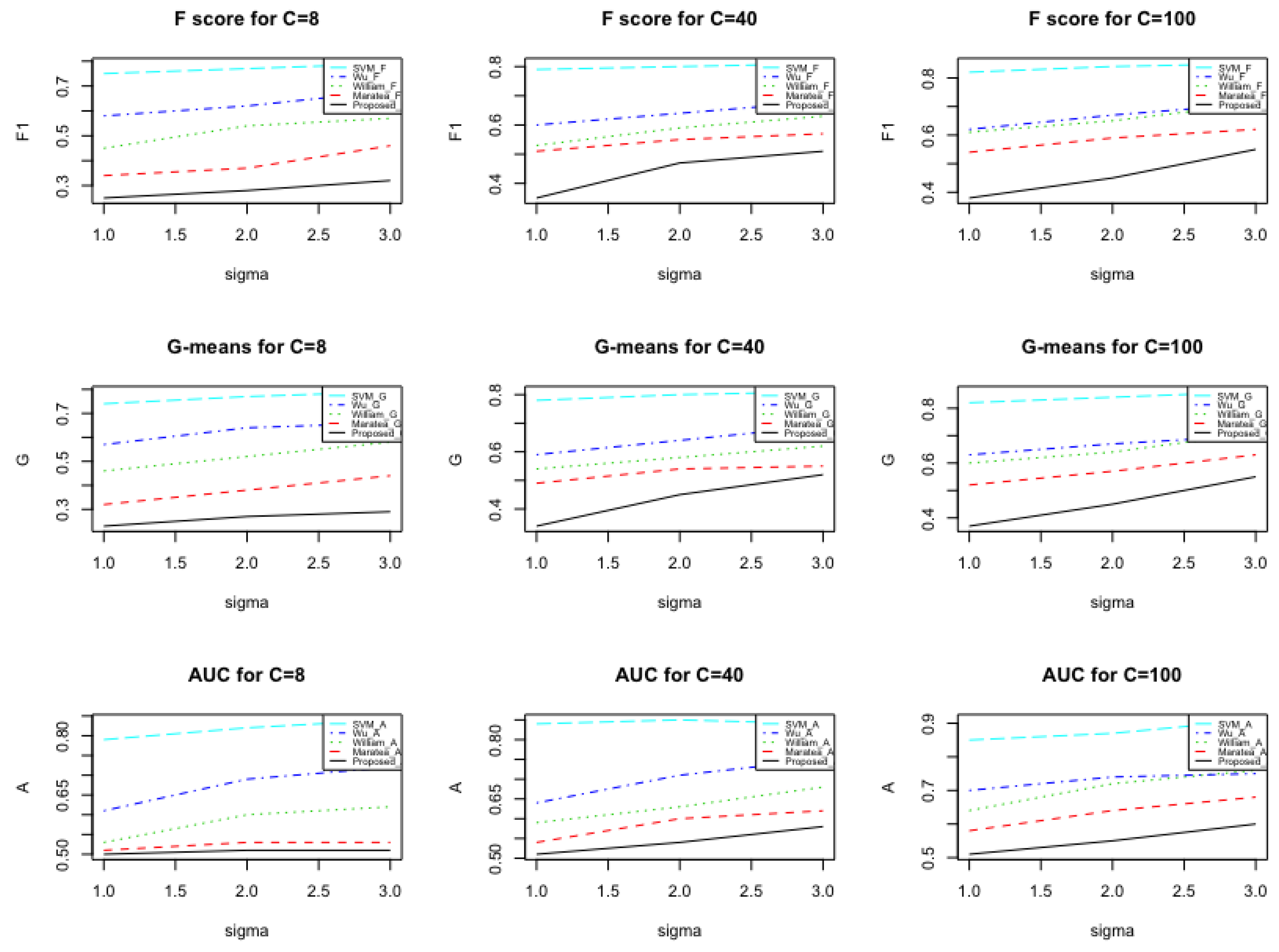
3.1. Simulation Study

First, we conduct simulation studies to evaluate the performance of the proposed method and compare it with the competitors in the literature. Three scenarios are considered. Each of them includes the balanced, moderately imbalanced, and extremely imbalanced cases, respectively. The Gaussian RBF kernel is employed during the first round of classification, if not mentioned elsewhere.

For convenience, the input space is 2-dimensional, and all training data are generated using three classes of bivariate Gaussian distributions with means vectors $(2,2),(4,3),(3,2)$, and identical covariance matrix $\gamma ·\Sigma$, where $\gamma$ is a nuisance parameter that controls the overlapping proportion of the classes. Moderate covariance is incorporated for all pairs with a correlation coefficient $\rho =0.3$, and the variance of all variables is 1.

The overall sample size for the training data is set as 600 and is separated into three classes by different weights in three different scenarios. The class size is $(200,200,200)$ in Scenario 1, $(100,200,300)$ in Scenario 2, and $(20,100,480)$ in Scenario 3. In each scenario, different combinations of parameters that need to be tuned will be considered. The cost parameter C is chosen from the set $\{0.1,0.2,0.5,1,5,8,40,100,500\}$ and $\sigma$ takes value from the set $\{0.01,0.05,0.1,0.5,1,5,10,100\}$. As Q is the threshold controlling the size of the local neighborhood, it is chosen by a grid search from the set $\{0.1,0.2,\dots ,1\}$ times the maximal Euclidean distance between all pairs of data points in the sample. All classifiers are tuned properly with respect to the corresponding measures.

The classification procedure is as follows. First, we train the classifiers with the traditional SVM using the one-versus-all strategy, and the support vectors are identified approximately. The kernel functions for all the methods are then updated adaptively by conformal transformation with different scalar function $c\left(\mathbf{x}\right)$, using $p_m$ defined in (21). A second round of SVM is then conducted, and the estimated class labels for observations in the test sample will be given and consequently compared with the true labels. Five-fold cross validation is employed to obtain the misclassification rate for each simulated dataset, and the whole process is repeated 1000 times. With the accuracy measures defined above, the performance of all the classifiers is shown in

Table 1. F-score (F), G-mean (G) and the AUC (A) measures for all five classification methods in Scenario 1 for $n_1=200$, $n_3=200$ and $n_3=200$, respectively. Max margin is 0.02.

		SVM				Wu [22]				William [23]				Maratea [24]				Our Method
$\mathit{C}$	$\mathit{\sigma }$	F	G	A		F	G	A		F	G	A		F	G	A		F	G	A
8	0.1	0.39	0.38	0.52		0.43	0.43	0.54		0.59	0.59	0.61		0.71	0.70	0.75		0.78	0.79	0.80
8	0.5	0.43	0.42	0.55		0.47	0.46	0.56		0.66	0.66	0.69		0.75	0.75	0.78		0.81	0.81	0.83
8	5.0	0.47	0.46	0.56		0.53	0.52	0.59		0.68	0.68	0.72		0.78	0.77	0.81		0.84	0.83	0.85
40	0.1	0.45	0.45	0.55		0.44	0.43	0.54		0.61	0.61	0.66		0.73	0.72	0.75		0.81	0.81	0.85
40	0.5	0.53	0.52	0.57		0.51	0.50	0.55		0.67	0.67	0.71		0.75	0.75	0.78		0.84	0.83	0.88
40	5.0	0.56	0.55	0.59		0.62	0.62	0.67		0.71	0.72	0.78		0.78	0.78	0.81		0.86	0.86	0.88
100	0.1	0.52	0.51	0.57		0.61	0.59	0.62		0.64	0.63	0.68		0.78	0.79	0.81		0.84	0.85	0.88
100	0.5	0.60	0.58	0.62		0.67	0.65	0.69		0.77	0.67	0.76		0.79	0.80	0.83		0.86	0.86	0.90
100	5.0	0.69	0.66	0.71		0.71	0.70	0.73		0.79	0.72	0.80		0.81	0.82	0.84		0.88	0.88	0.92

,

Table 2. F-score (F), G-mean (G) and the AUC (A) measures for all five classification methods in Scenario 2 for $n_1=100$, $n_3=200$ and $n_3=300$, respectively. Max margin is 0.04.

		SVM				Wu [22]				William [23]				Maratea [24]				Our Method
$\mathit{C}$	$\mathit{\sigma }$	F	G	A		F	G	A		F	G	A		F	G	A		F	G	A
8	0.1	0.29	0.30	0.51		0.40	0.40	0.52		0.49	0.49	0.55		0.62	0.60	0.63		0.77	0.76	0.80
8	0.5	0.32	0.32	0.51		0.42	0.42	0.55		0.58	0.57	0.63		0.66	0.65	0.71		0.78	0.78	0.82
8	5.0	0.36	0.36	0.52		0.48	0.49	0.55		0.61	0.60	0.67		0.71	0.72	0.77		0.80	0.80	0.84
40	0.1	0.40	0.40	0.54		0.54	0.53	0.57		0.57	0.58	0.62		0.65	0.66	0.71		0.80	0.80	0.83
40	0.5	0.50	0.42	0.52		0.59	0.58	0.64		0.65	0.64	0.69		0.68	0.67	0.73		0.81	0.80	0.85
40	5.0	0.56	0.56	0.61		0.62	0.60	0.64		0.68	0.66	0.72		0.72	0.73	0.77		0.82	0.82	0.88
100	0.1	0.42	0.39	0.54		0.57	0.55	0.61		0.65	0.64	0.69		0.66	0.68	0.75		0.84	0.83	0.88
100	0.5	0.52	0.50	0.59		0.63	0.65	0.71		0.70	0.69	0.75		0.71	0.72	0.77		0.85	0.84	0.89
100	5.0	0.59	0.61	0.66		0.68	0.70	0.74		0.75	0.76	0.79		0.75	0.74	0.81		0.86	0.87	0.91

and

Table 3. F-score (F), G-mean (G) and the AUC (A) measures for all five classification methods in Scenario 3 for $n_1=20$, $n_3=100$ and $n_3=480$, respectively. Max margin is 0.05.

		SVM				Wu [22]				William [23]				Maratea [24]				Our Method
$\mathit{C}$	$\mathit{\sigma }$	F	G	A		F	G	A		F	G	A		F	G	A		F	G	A
8	0.1	0.25	0.23	0.50		0.34	0.32	0.51		0.45	0.46	0.53		0.58	0.57	0.61		0.75	0.74	0.79
8	0.5	0.28	0.27	0.51		0.37	0.38	0.53		0.54	0.52	0.60		0.62	0.64	0.69		0.77	0.77	0.82
8	5.0	0.32	0.29	0.51		0.46	0.44	0.53		0.57	0.58	0.62		0.68	0.66	0.72		0.79	0.79	0.84
40	0.1	0.35	0.34	0.51		0.51	0.49	0.54		0.53	0.54	0.59		0.60	0.59	0.64		0.79	0.78	0.84
40	0.5	0.47	0.45	0.54		0.55	0.54	0.60		0.59	0.58	0.63		0.64	0.64	0.71		0.80	0.80	0.85
40	5.0	0.51	0.52	0.58		0.57	0.55	0.62		0.63	0.62	0.68		0.68	0.69	0.75		0.81	0.81	0.84
100	0.1	0.38	0.37	0.51		0.54	0.52	0.58		0.61	0.60	0.64		0.62	0.63	0.70		0.82	0.82	0.85
100	0.5	0.45	0.45	0.55		0.59	0.57	0.64		0.65	0.64	0.72		0.67	0.67	0.74		0.84	0.84	0.87
100	5.0	0.55	0.55	0.60		0.62	0.63	0.68		0.71	0.71	0.76		0.71	0.70	0.75		0.85	0.86	0.91

, and Figure 1, Figure 2 and Figure 3. Similar results are seen in the proposed method with the other way of defining $p_m$.

It is seen that all methods considered here have improved performances comparing to the ordinary SVM in almost all scenarios with different combinations of the parameters C and $\sigma$. In general, the proposed method outperforms all the other classifiers considered, especially in the imbalanced data. When $\sigma$ gets larger with fixed C, the misclassification rate tends to decrease in all the methods compared. When $\sigma$ is relatively small, the proposed method performs better than those of Wu and Williams’ methods, while if $\sigma$ is relatively large, all the methods are nearly the same. This is because when $\sigma$ is large, the feasible solution set gets large, and all of the methods tend to find the optimal solution. Correspondingly, when C increases, the budget for misclassification gets bigger, which means more tolerance is permitted so that the two classes can be separated. In this scenario, we found that $p_m$ is roughly the same, approximately the reciprocal of ${\left|D\right|}_{max}$. This makes sense because in the balanced-data case, the density of the distributed SVs is roughly uniform, and hence the averages of the distance in the feature space for each data point are roughly the same.

For imbalanced scenarios the performances of all methods turn out to be a bit worse than the balanced case with no surprise due to the non-uniformly distributed support vectors. The change of the misclassification rate with C and $\sigma$ is similar to that in the balanced data case. The proposed method performs the best among all the methods.

3.2. A Real Prostate Caner MRI Dataset

In this section, we apply the proposed method to a prostate cancer MR image dataset. The study aims to find statistical methods to classify cancer and non-cancer areas or grades of cancer by the imaging data obtained by imaging collection equipments. In this case, nine common classes are labeled and listed as follows, indicating different levels of severity of cancer.

• Atrophy: As means literally (non-cancer);
• EPE: Prostatic intraepithelial neoplasia (non-cancer);
• PIN: Prostatic intraepithelial neoplasia (non-cancer);
• G3: Tumour focus that is all Gleason 3 (cancer);
• G4: Tumour focus that is all Gleason 4 (cancer);
• G3+4: Tumour focus all predominately G3 with intermingled G4 (cancer);
• G4+3: Tumour focus all predominately G4 with intermingled G3 (cancer);
• G4+5: Tumour focus all predominately G4 with intermingled G5 (cancer);
• OtherProstate: Prostate tissue that does not fall into the other categories (non-cancer).

Note that the labels are given at the voxel level. That is, for a specific patient, it is very likely to have different voxels (indicating different positions of the prostate tissue) with different classes. A patient that has $G3+4$-type cancer in some areas is likely to have $G3$-type cancer as well as $OtherProstate$-type of voxels in other areas. Our objective is to predict class labels at the voxel level. There are several labels associated with $G5$, however, the whole dataset contains only one patient with a very tiny area of $G5$ and the associated type of cancer. Therefore, $G5$ is extremely imbalanced.

In the first phase of the study, 21 patients are involved and more than 400 images are collected. Predictors on each voxel are the three-dimensional intensity measures from MRIs, denoted as T2W intensity, ADC intensity and C-Grade intensity. Other measures such as DCE and DWI are only available to part of the patients and hence are not included in the training process.

To adopt the proposed data-adaptive scaling in this multi-class case, two-stage SVMs are required. During the first stage, a standard SVM with the selected kernel is conducted so that the support vectors from the original dataset can be found. Based on the identified support vectors, the kernel functions are updated. Then, a second-stage SVM is conducted with the updated kernel, and the resulting estimated boundary will be used as the rule for classification. In terms of choosing appropriate tuning parameters for each method, 7-fold cross validation is conducted for 500 times at the patient level.

To assess the performance, we compare our proposed methods with both traditional and data-adaptive multi-category classification methods. In terms of the traditional methods, one-versus-one (1vs1) and one-versus-all (1vsA) from indirect methods, and the Crammer and Singer’s (CS) direct methods and He’s Simplified SVM (simSVP) will be included, while for the data-adaptive methods, Amari’s and William’s adaptively scaling will be included. In terms of the criterion of the classification performance, misclassification rate, percentage of support vectors in the whole dataset, F-score and G-means along with their margins are reported.

Table 4. Outcomes of multi-class prediction on the Prostate Cancer Program.

Methods	Error(%)	SV(%)	F-Score	G-Means
Proposed	$8.06\pm 0.58$	$17.46\pm 0.57$	$0.84\pm 0.05$	$0.81\pm 0.04$
Amari	$11.88\pm 1.12$	$21.33\pm 1.27$	$0.70\pm 0.09$	$0.66\pm 0.10$
William	$10.21\pm 0.97$	$18.93\pm 1.65$	$0.74\pm 0.12$	$0.71\pm 0.08$
CS	$9.20\pm 1.22$	$17.57\pm 1.12$	$0.77\pm 0.06$	$0.73\pm 0.06$
simSVM	$9.33\pm 1.20$	$18.29\pm 1.07$	$0.78\pm 0.10$	$0.74\pm 0.09$
1vs1	$8.20\pm 1.26$	$25.41\pm 2.87$	$0.81\pm 0.06$	$0.77\pm 0.07$
1vsA	$8.25\pm 1.57$	$24.16\pm 2.62$	$0.82\pm 0.06$	$0.76\pm 0.06$

presents the assessment measures for all the methods considered. Obviously, the proposed method performs almost the best among all the compared methods. A highlight point is that the proposed method has the smallest margins in all performance measures, resulting from the property of the robust decay of the magnification effect from the proposed data-adaptive kernel. In terms of the accuracy, the proposed method has a similar misclassification rate to the indirect methods, which is significantly smaller than the rest of the methods. F-score and G-means are the largest for the proposed method, much larger than other data-adaptive kernel methods. The percentage of support vectors that are used for constructing the classifiers is the smallest for the proposed method.

It is worth pointing out that among those wrongly predicted labels, $G4+3$ is the dominant class. In other words, the misclassification always happens in $G4+3$ type cancer. This is because this type of cancer is really rare in the training sample, taking only 1–2% among all the labels. These extremely imbalanced data have made it very difficult to be detected with a high accuracy. The proposed method can detect around 60% among this type, while other data adaptive (Amari’s and William’s) methods can only find less than 20%. All other methods cannot detect this class. Also, only our method detects the $G5$ class from the only one patient, while all competitor methods fail.

4. Concluding Remarks

In this paper, we developed a new data-dependent SVM construction technique for the multi-category classification problem. Based on the data-adaptive kernel SVM for the binary case, we proposed a new method to construct the data-dependent kernel for the multi-class setting, especially when the data are imbalanced. The data-dependent kernel functions have a more robust decay rate and can vary along with the density of the size of neighbors. Thus, the kernel can be adapted optimally for a specific dataset. Numerical results from both synthetic and real datasets have shown the excellent performance of the proposed method. Not only does the proposed method outperform in terms of the commonly used accuracy measures such as the F-score and G-means, compared with the competitors, but also successfully detects more than 60% of instances from the rare class in the real data, while the competitors can only detect less than 20%. A possible future work is to select relevant predictors for the multi-class kernel functions and consider the spatial association between different images. It is worth noting that the misclassification rate will be affected by the distance of the mean vectors. For instance, the misclassification will not occur if the centers of the three Gaussian distributions are sufficiently far from each other when the covariance matrix is set as unity. The proposed method may be useful in other scientific research fields, such as detecting the boundaries of multiple regions of interest.

References

1. Liu, X.; He, W. Adaptive kernel scaling support vector machine with application to a prostate cancer image study. J. Appl. Stat. 2021, 1–20. [Google Scholar] [CrossRef]
2. Crammer, K.; Singer, Y. On the algorithmic implementation of multiclass kernel-based vector machines. J. Mach. Learn. Res. 2001, 2, 265–292. [Google Scholar]
3. Maratea, A.; Petrosino, A. Asymmetric Kernel scaling for imbalanced data classification. Fuzzy Log. Appl. 2011, 196–203. [Google Scholar] [CrossRef]
4. Zhang, Z.; Gao, G.; Shi, Y. Credit risk evaluation using multi-criteria optimization classifier with kernel, fuzzification and penalty factors. Eur. J. Oper. Res. 2014, 237, 335–348. [Google Scholar] [CrossRef]
5. Vapnik, V.N.; Vapnik, V. Statistical Learning Theory; Wiley: New York, NY, USA, 1998; Volume 1. [Google Scholar]
6. Menardi, G.; Torelli, N. Training and assessing classification rules with imbalanced data. Data Min. Knowl. Discov. 2014, 28, 92–122. [Google Scholar] [CrossRef]
7. Kreßel, U.H.G. Pairwise classification and support vector machines. In Advances in Kernel Methods; MIT Press: Cambridge, MA, USA, 1999; pp. 255–268. [Google Scholar]
8. Suykens, J.A.; Vandewalle, J. Least squares support vector machine classifiers. Neural Process. Lett. 1999, 9, 293–300. [Google Scholar] [CrossRef]
9. Suykens, J.A.; Vandewalle, J. Multiclass least squares support vector machines. In Proceedings of the International Joint Conference on Neural Networks, IJCNN’99, Washington, DC, USA, 10–16 July 1999; Volume 2, pp. 900–903. [Google Scholar]
10. Xia, X.L.C.; Li, K. A sparse multi-class least-squares support vector machine. In Proceedings of the IEEE International Symposium on Industrial Electronics, Cambridge, UK, 30 June–2 July 2008; pp. 1230–1235. [Google Scholar]
11. Fung, G.M.; Mangasarian, O.L. Multicategory proximal support vector machine classifiers. Mach. Learn. 2005, 59, 77–97. [Google Scholar] [CrossRef] [Green Version]
12. Fung, G.M.; Mangasarian, O. Proximal support vector machine classifiers. Mach. Learn. 2002, 1, 21. [Google Scholar]
13. Zhang, Y.; Fu, P.; Liu, W.; Chen, G. Imbalanced data classification based on scaling kernel-based support vector machine. Neural Comput. Appl. 2014, 25, 927–935. [Google Scholar] [CrossRef]
14. He, X.; Wang, Z.; Jin, C.; Zheng, Y.; Xue, X. A simplified multi-class support vector machine with reduced dual optimization. Pattern Recognit. Lett. 2012, 33, 71–82. [Google Scholar] [CrossRef]
15. Mazurowski, M.A.; Habas, P.A.; Zurada, J.M.; Lo, J.Y.; Baker, J.A.; Tourassi, G.D. Training neural network classifiers for medical decision making: The effects of imbalanced datasets on classification performance. Neural Netw. 2008, 21, 427–436. [Google Scholar] [CrossRef] [PubMed] [Green Version]
16. Chawla, N.; Japkowicz, N.; Kolcz, A. Special Issue on Learning from Imbalanced Datasets, Sigkdd Explorations; ACM SIGKDD: New York, NY, USA, 2004; Volume 6, pp. 1–6. [Google Scholar]
17. Daskalaki, S.; Kopanas, I.; Avouris, N. Evaluation of classifiers for an uneven class distribution problem. Appl. Artif. Intell. 2006, 20, 381–417. [Google Scholar] [CrossRef]
18. Chawla, N.V.; Japkowicz, N.; Kotcz, A. Editorial: Special issue on learning from imbalanced data sets. ACM Sigkdd Explor. Newsl. 2004, 6, 1–6. [Google Scholar] [CrossRef]
19. Tang, Y.; Zhang, Y.Q.; Chawla, N.V.; Krasser, S. SVMs modeling for highly imbalanced classification. Syst. Man Cybern. Part B Cybern. IEEE Trans. 2009, 39, 281–288. [Google Scholar] [CrossRef] [PubMed] [Green Version]
20. Wang, L.; Shen, X. On L1-norm multiclass support vector machines. J. Am. Stat. Assoc. 2007, 102, 583–594. [Google Scholar] [CrossRef]
21. Friedman, J.; Hastie, T.; Tibshirani, R. The Elements of Statistical Learning; Springer Series in Statistics; Springer: Berlin/Heidelberg, Germany, 2001; Volume 1. [Google Scholar]
22. Wu, S.; Amari, S.I. Conformal transformation of kernel functions: A data-dependent way to improve support vector machine classifiers. Neural Process Lett. 2002, 15, 59–67. [Google Scholar] [CrossRef]
23. Williams, P.; Li, S.; Feng, J.; Wu, S. Scaling the kernel function to improve performance of the support vector machine. In Advances in Neural Networks–ISNN 2005; Springer: Berlin/Heidelberg, Germany, 2005; pp. 831–836. [Google Scholar]
24. Maratea, A.; Petrosino, A.; Manzo, M. Adjusted F-measure and kernel scaling for imbalanced data learning. Inf. Sci. 2014, 257, 331–341. [Google Scholar] [CrossRef]
25. Fawcett, T. ROC graphs: Notes and practical considerations for researchers. Mach. Learn. 2004, 31, 1–38. [Google Scholar]
Figure 1. Performance of the competitor methods for Scenario 1.
Mathematics 09 00936 g001
Figure 2. Performance of the competitor methods for Scenario 2.
Mathematics 09 00936 g002
Figure 3. Performance of the competitor methods for Scenario 3.
Mathematics 09 00936 g003