The Heston Model with Time-Dependent Correlation Driven by Isospectral Flows

Abstract

In this work, we extend the Heston stochastic volatility model by including a time-dependent correlation that is driven by isospectral flows instead of a constant correlation, being motivated by the fact that the correlation between, e.g., financial products and financial institutions is hardly a fixed constant. We apply different numerical methods, including the method for backward stochastic differential equations (BSDEs) for a fast computation of the extended Heston model. An example of calibration to market data illustrates that our extended Heston model can provide a better volatility smile than the Heston model with other considered extensions.

1. Introduction

The Heston model [1] is one of the most widely used affine stochastic volatility models for equity prices, which is an extension of the Black and Schloes model [2] by taking into account stochastic volatility that is driven by a Cox-Ingersoll-Ross (CIR) process [3]. However, it is well-known that, in many cases, the Heston model cannot provide enough skews or smiles in the implied volatility as market requires, in particular with short maturity. To tackle this problem, several extensions have been proposed in the literature: the Heston model by allowing time-dependent parameters [4,5,6]; the double Heston model with an additional volatility process [7]; the Heston model extended with a stochastic interest rate [8]; the Heston model that is extended by imposing a stochastic correlation [9,10]; and, the Heston model with a time-dependent correlation function [11]. The contribution of this work can be categorized into the class of extensions by including a time-dependent correlation. Our aim is to improve the pure Heston model to provide better smiles in the implied volatility as market requires, and to add an economic concept of nonlinear relationship between the asset and its volatility.

In [11], a novel time-dependent correlation function has been embedded into the Heston model, four additional parameters (compared to the pure Heston model) are gained to increase the fitting quality. However, that time-dependent model is semi-analytical with numerical integral, i.e., more computational complexity. In this work, we improve the Heston model by including a novel correlation flow that is given in an analytical form in the context of isospectral flow [12]. Using this new method, one can arbitrarily add many additional parameters to improve the fitting quality on one hand but also add an economic concept (nonlinear relationship) on the other hand. Furthermore, the time-dependent correlation matrix that is embedded in the Heston model is valid at each time instance, i.e.,

• all diagonal elements are equal to one and absolute values of all non-diagonal elements are less than one,
• non-negative eigenvalues (positive semidefinite).

Furthermore, we show how to represent the extended Heston model by a (two-dimensional) backward stochastic differential equations (BSDEs), and solve them using numerical method for BSDEs, e.g., [13]. We also fit our new model to a real market data, and show the better performance than that in [11].

The outline of the remaining part is as follows. In the next section, we introduce the correlation flow. Section 3 is devoted to the specification of a correlation flow for the Heston model. In Section 4, we incorporate the correlation flow into the Heston model, and represent the extended model by a BSDE. Section 5 illustrates the calibration. Finally, in Section 6 we conclude.

2. The Correlation Flows

In this section, we first review the idea of covariance and correlation flows proposed in Teng, L.; Wu, X.; Günther, M.; Ehrhardt, M. 2020 [12]. Following that idea, we propose a new correlation flow and extend the Heston model by including that correlation flow.

Let $\mathcal{G}$ be the Lie group of all non-singular matrices in ${\mathbb{R}}^{n\times n},$ and $X_0\in {\mathbb{R}}^{n\times n}$ be given. An isospectral surface is defined by

$$\mathcal{M}\left(X_0\right):=\left\{Z^{-1}{X}_{0}Z|Z\in \mathcal{G}\left(n\right)\right\}.$$

From now on we consider the subgroup $\mathcal{O}\left(n\right)$ of all orthogonal matrices and define

$$\tilde{\mathcal{M}}\left(P_0\right):=\left\{Q^{-1}{P}_{0}Q|Q\in {\mathcal{O}}_n\right\},$$

and start with the following main theorem, which can be used to define isospectral curves.

Theorem 1

([12]). Given that $Q\left(t\right),$ with $Q\left(0\right)=I$ (Identity matrix), represents a differential curve on the manifold $\mathcal{O}\left(n\right).$ It holds that

$$P\left(t\right)=Q{\left(t\right)}^{\top }{P}_{0}Q\left(t\right),$$

(1)

which is the solution (upon differentiation) of the initial value problem

$$\left\{\begin{array}{c}\hfill \frac{dP\left(t\right)}{dt}=[P\left(t\right),k\left(t\right)],t\ge 0\hfill \\ \hfill P\left(0\right)=P_0,\hfill \end{array}\right.$$

(2)

where, for $t\ge 0,$ $\left[P\right(t),k(t\left)\right]=P\left(t\right)k\left(t\right)-k\left(t\right)P\left(t\right)$ denotes the Lie bracket and $k\left(t\right)$ is defined by

$$k\left(t\right):=Q{\left(t\right)}^{\top }\frac{dQ\left(t\right)}{dt},t\ge 0.$$

(3)

Note that (1) defines a differentiable curve on the surface $\stackrel{\sim }{\mathcal{M}}\left(P_0\right)$ with $P\left(0\right)=P_0.$ Furthermore, if $k\left(t\right)\in {\mathbb{R}}^{n\times n}$ is known, the differentiable curve (1) can be obtained by solving (2). We see that the solution of (2) can be formulated in the form of (1), where $Q\left(t\right)$ satisfies

$$\left\{\begin{array}{c}\hfill \frac{dQ\left(t\right)}{dt}=Q\left(t\right)k\left(t\right),t\ge 0\hfill \\ \hfill Q\left(0\right)=I.\hfill \end{array}\right.$$

(4)

By using (2) with different values of $k\left(t\right)$, one can define different isospectral curves.

Obviously, the aim is to create covariance flows ${\left(P\left(t\right)\right)}_{t\in {\mathbb{R}}_{+}},$ which must be valid, i.e., positive semi-definite for all $t\ge 0.$ With the aid of the singular value decomposition (SVD), we obtain

$$P\left(t\right)=\tilde{Q}{\left(t\right)}^{\top }S\left(t\right)\tilde{Q}\left(t\right),$$

(5)

where $S\left(t\right)$ is a diagonal matrix that consists of singular values of $P\left(t\right)$ and $\tilde{Q}\left(t\right)$ is a unitary matrix consisting of singular vectors. Without a loss of generality, we assume that $\tilde{Q}\left(t\right)$ is a rotation matrix whose determinant is always $1.$ Because the covariance flows are modelled as the isospectral flows, they then must have the same singular values for $t\ge 0.$ Therefore, (5) can be given via (1) as

$$P\left(t\right)=\tilde{Q}{\left(t\right)}^{\top }S\left(t\right)\tilde{Q}\left(t\right):=Q{\left(t\right)}^{\top }\underset{:=P\left(0\right)}{\underbrace{Q{\left(0\right)}^{\top }S\left(0\right)Q\left(0\right)}}Q\left(t\right),$$

by which a valid covariance flow can be created with the given initial value $P_0$ and rotation matrices $Q\left(t\right).$ Obviously, a valid corresponding correlation flow can be obtained by converting the covariance flow.

3. Time-Dependently Correlated Brownian Motions (BMs) via Flow

We fix a probability space $(\mathrm{\Omega },\mathcal{F},\mathbb{P})$ and an information filtration ${\left({\mathcal{F}}_t\right)}_{t\in {\mathbb{R}}^{+}}$, satisfying the usual conditions, see e.g., Øksendal, B. 2003 [14]. At a time $t>0,$ the correlation coefficient of two Brownian motions (BMs) $W_t^1$ and $W_t^2$ is defined as

$${\rho }^{1,2}\left(t\right)=\frac{E\left[W_t^1{W}_t^2\right]}{t}.$$

If one assumes that ${\rho }^{1,2}\left(t\right)$ is constant, ${\rho }_t^{1,2}={\rho }^{1,2}$ for all $t>0$, say $W_t^1\mathrm{a}\mathrm{n}\mathrm{d}{W}_t^2$ are correlated with the constant ${\rho }^{1,2}.$

Therefore, we give the definition of time-dependently correlated BMs.

Definition 1.

Teng, L.; Günther, M.; Ehrhardt, M. 2016 [11] Two Brownian motions $W_t^1$ and $W_t^2$ are called dynamically correlated with correlation function $\rho \left(t\right),$ if they satisfy

$$E\left[W_t^1{W}_t^2\right]={\int }_0^t\rho \left(s\right)ds,$$

where $\rho \left(t\right):[0,t]\to [-1,1].$ The average correlation of $W_t^1$ and $W_t^2$, ${\rho }_{Av},$ is given by ${\rho }_{Av}:=\frac{1}{t}{\int }_0^t\rho \left(s\right)ds.$

In [12], the authors show how to construct $Q\left(t\right),$ namely $k\left(t\right)$, as given in (3) for both the cases whether $k\left(t\right)$ and ${\int }_0^{t}k\left(s\right)ds$ are commutative or non-commutative. We propose a new correlation flow in the commutative case, and then apply it into the Heston model. Suppose that the initial correlation matrix $\rho \left(0\right)$ and standard deviations ${\sigma }^S,{\sigma }^{\nu }$ are given, which can be converted to the initial covariance matrix

$$P\left(0\right):=P_0=\left(\begin{array}{cc}{\left({\sigma }^S\right)}^2& \rho \left(0\right){\sigma }^S{\sigma }^{\nu }\\ \rho \left(0\right){\sigma }^S{\sigma }^{\nu }& {\left({\sigma }^{\nu }\right)}^2\end{array}\right).$$

(6)

Let

$${\int }_0^{t}k\left(s\right)ds=(\alpha t+\cos (\beta t+\cos \left(\zeta t\right))+2\pi n)\left(\begin{array}{cc}0& -1\\ 1& 0\end{array}\right),$$

which is skew-symmetric, where n is an integer. Thus, we see that the unique solution of (4) is given by

$$Q\left(t\right)={\mathrm{e}}^{{\int }_0^{t}k\left(s\right)ds}=\left(\begin{array}{cc}\cos (\alpha t+\cos (\beta t+\cos \left(\zeta t\right)\left)\right)& -\sin (\alpha t+\cos (\beta t+\cos \left(\zeta t\right)\left)\right)\\ \sin (\alpha t+\cos (\beta t+\cos \left(\zeta t\right)\left)\right)& \cos (\alpha t+\cos (\beta t+\cos \left(\zeta t\right)\left)\right)\end{array}\right),$$

(7)

which are rotation matrices. Thus, the covariance flow can be defined as

$$P\left(t\right)=Q{\left(t\right)}^{\top }{P}_{0}Q\left(t\right),$$

(8)

where $P_0$ and $Q\left(t\right)$ are given in (6) and (7), respectively. Finally, the correlation flow can be obtained by converting the latter covariance flow, which is denoted by ${\left(\rho \left(t\right)\right)}_{t\in {\mathbb{R}}_{+}}$ and used in the sequel.

For two independent BMs $W_t^1\mathrm{a}\mathrm{n}\mathrm{d}{W}_t^3$, we define

$$W_t^2={\int }_0^t\rho \left(s\right)d{W}_s^1+{\int }_0^t\sqrt{1-{\rho }^2\left(s\right)}d{W}_s^3,$$

with the symbolic expression

$$d{W}_t^2=\rho \left(t\right)d{W}_t^1+\sqrt{1-{\rho }^2\left(t\right)}d{W}_t^3.$$

It can be easily verified that $W_t^2$ is a BM and correlated with $W_t^1$ time-dependently by $\rho \left(t\right),$ namely

$$d{W}_t^{1}d{W}_t^2=\rho \left(t\right)dt$$

Note that, in our setting above, the correlation flow is specified with 6 parameters, which are ${\rho }_0,{\sigma }^S,{\sigma }^{\nu },\alpha ,\beta$ and $\zeta .$ However, more parameters can be included for a better fitting, e.g., setting

$${\int }_0^{t}k\left(s\right)ds=({\alpha }_{1}t+\cos ({\alpha }_{2}t+\cos ({\alpha }_{3}t+\cdots +\cos \left({\alpha }_{m}t\right)\cdots ))+2\pi N)\left(\begin{array}{cc}0& -1\\ 1& 0\end{array}\right).$$

for $N+3$ parameters.

4. The Heston Model with Correlation Flow

The pure Heston’s stochastic volatility model is specified as

$$\begin{array}{ccc}\hfill d{S}_t& =& \hfill {\mu }_S{S}_{t}dt+\sqrt{{\nu }_t}{S}_{t}d{W}_t^S,\hfill \end{array}$$

(9)

$$\begin{array}{ccc}\hfill d{\nu }_t& =& \hfill {\kappa }_{\nu }({\mu }_{\nu }-{\nu }_t)dt+{\sigma }_{\nu }\sqrt{{\nu }_t}d{W}_t^{\nu },\hfill \end{array}$$

(10)

where $S_t$ is the spot price of the underlying asset, ${\nu }_t$ is the volatility (variance), and the Brownian motions $W_t^S\mathrm{a}\mathrm{n}\mathrm{d}{W}_t^{\nu }$ are correlated by the constant correlation ${\rho }_{S\nu }$. To include a time-dependent correlation, we let $d{S}_t\mathrm{a}\mathrm{n}\mathrm{d}d{\nu }_t$ be related with the time-dependent correlation $\rho \left(t\right)$ instead of ${\rho }_{S\nu }.$ Therefore, the Heston model extended with time-dependent correlation $\rho \left(t\right)$ is defined as

$$\begin{array}{cc}\hfill d{S}_t& \hfill ={\mu }_S{S}_{t}dt+\sqrt{{\nu }_t}{S}_{t}d{\tilde{W}}_t^S,\hfill \\ \hfill d{\nu }_t& \hfill ={\kappa }_{\nu }({\mu }_{\nu }-{\nu }_t)dt+{\sigma }_{\nu }\sqrt{{\nu }_t}(\rho \left(t\right)d{\tilde{W}}_t^S+\sqrt{1-{\rho }^2\left(t\right)}d{\tilde{W}}_t^{\nu }),\hfill \end{array}$$

(11)

where ${\tilde{W}}_t^S\mathrm{a}\mathrm{n}\mathrm{d}{\tilde{W}}_t^{\nu }$ are independent. In this work, we consider, e.g., a European call option with strike price K and maturity $T,$ and solve (11) numerically using BSDE-based Teng, L. 2019 [13] and ODE-based [11] methods.

4.1. The BSDE-Based Numerical Approximation

The BSDE for the pure Heston model is derived in [13]:

$$\begin{array}{cc}\hfill -d{Y}_t& \hfill =\left(-\frac{\lambda \sqrt{{\nu }_t}}{{\sigma }_{\nu }}{Z}_t^1+\left(\frac{\rho \lambda \sqrt{{\nu }_t}}{\sqrt{1-{\rho }^2}{\sigma }_{\nu }}-\frac{({\mu }_S-r)}{\sqrt{1-{\rho }^2}\sqrt{{\nu }_t}}\right)Z_t^2-r{Y}_t\right)dt-{\mathbf{Z}}_t\left(\begin{array}{c}d{\tilde{W}}_t^{\nu }\\ d{\tilde{W}}_t^S\end{array}\right)\hfill \end{array}$$

with ${\mathbf{Z}}_t=(Z_t^1,Z_t^2),$ where r is the interest rate, $\lambda$ is the parameter for the market price of the volatility risk as that in [1], and ${\tilde{W}}_t^{\nu }$ and ${\tilde{W}}_t^S$ are independent BMs. Let $Y_T=max(S_T-K,0),$ $Y_t$ is thus the Heston option value $V(t,S_t,{\nu }_t,{\rho }_{S\nu }),$ and ${\mathbf{Z}}_t$ presents the hedging strategies with $(Z_t^1,Z_t^2)=\left(\frac{\partial V}{\partial \nu }{\sigma }_{\nu }\sqrt{{\nu }_t}+\frac{\partial V}{\partial S}{S}_t\rho \sqrt{{\nu }_t},\frac{\partial V}{\partial S}{S}_t\sqrt{1-{\rho }^2}\sqrt{{\nu }_t}\right).$ Analogously, the corresponding BSDE for the extended Heston model in (11) can be directly adopted as

$$-d{Y}_t=\left(-\frac{\tilde{\lambda }\sqrt{{\nu }_t}}{{\sigma }_{\nu }}{Z}_t^1+\left(\frac{\rho \left(t\right)\tilde{\lambda }\sqrt{{\nu }_t}}{\sqrt{1-{\rho }^2\left(t\right)}{\sigma }_{\nu }}-\frac{({\mu }_S-r)}{\sqrt{1-{\rho }^2\left(t\right)}\sqrt{{\nu }_t}}\right)Z_t^2-r{Y}_t\right)dt-{\mathbf{Z}}_t\left(\begin{array}{c}d{\tilde{W}}_t^{\nu }\\ d{\tilde{W}}_t^S\end{array}\right),$$

(12)

where the correlation flow $\rho \left(t\right)$ is constructed in the previous section, and with the parameters ${\rho }_0,{\sigma }^S,{\sigma }^{\nu },\alpha ,\beta$ and $\zeta .$ $\tilde{\lambda },$ which is the parameter for the market price of the volatility risk and depends also on the correlation flow, can be written as $\tilde{\lambda }(S,\nu ,\rho \left(t\right),t).$ This is to say that the price of correlation risk has been embedded in the price of volatility risk. The option value and corresponding hedging strategies are given by $Y_t=V(t,S_t,{\nu }_t,\rho \left(t\right))$ and $(Z_t^1,Z_t^2)=\left(\frac{\partial V}{\partial \nu }{\sigma }_{\nu }\sqrt{{\nu }_t}+\frac{\partial V}{\partial S}{S}_t\rho \left(t\right)\sqrt{{\nu }_t},\frac{\partial V}{\partial S}{S}_t\sqrt{1-\rho {\left(t\right)}^2}\sqrt{{\nu }_t}\right)$ for $Y_T=max(S_T-K,0),$ respectively. Finally, the two-dimensional BSDE shown in (12) can be solved using a BSDE-based numerical method, and we choose the regression tree-based approach in [13].

4.2. The ODE-Based Numerical Approximation

For comparative purposes, we also apply the method proposed in [11] to numerically solve (11). Applying Itô’s lemma and no-arbitrage argument, it yields [1]

$$\begin{array}{cc}\hfill \frac{1}{2}\nu S^2\frac{{\partial }^{2}U}{\partial S^2}& \hfill +\rho \left(t\right){\sigma }_{\nu }\nu S\frac{{\partial }^{2}U}{\partial S\partial \nu }+\frac{1}{2}{\sigma }_{\nu }^2\nu \frac{{\partial }^{2}U}{\partial {\nu }^2}+rS\frac{\partial U}{\partial S}\hfill \\ \hfill & \hfill +[{\kappa }_{\nu }({\mu }_{\nu }-\nu )-\tilde{\lambda }(S,\nu ,\rho \left(t\right),t)\nu ]\frac{\partial U}{\partial \nu }-rU+\frac{\partial U}{\partial t}=0.\hfill \end{array}$$

(13)

We consider, e.g., a European call option with maturity T and strike price K

$$V(S,\nu ,t,\rho \left(t\right))=S{P}_1-KP(t,T)P_2,\tau =T-t,$$

(14)

with the discount factor $P(t,T).$ We see that both the in-the-money probabilities $P_1,P_2$ must satisfy the PDE (13) as well as their characteristic functions that are defined by

$$f_j(S_t,{\nu }_t,\rho \left(t\right),\varphi ,t)=E\left[{\mathrm{e}}^{i\varphi ln{S}_T}\right|S_t,{\nu }_t,\rho \left(t\right)]={\mathrm{e}}^{C_j(\tau ,\varphi )+D_j(\tau ,\varphi )\nu +i\varphi ln{S}_t},j=1,2,$$

(15)

where $C_j(0,\varphi )=0$ and $D_j(0,\varphi )=0.$ We substitute (15) into the PDE (13) and, thus, obtain the following ordinary differential equations (ODEs) for the unknown functions $C\mathrm{a}\mathrm{n}\mathrm{d}D:$

$$\begin{array}{cc}\hfill -\frac{1}{2}{\varphi }^2+\rho \left(t\right){\sigma }_{\nu }\varphi i{D}_j+\frac{1}{2}{\sigma }_{\nu }^2{D}_j^2+u_j\varphi i-b_j{D}_j+\frac{\partial D_j}{\partial t}& \hfill =0,\hfill \end{array}$$

(16)

$$\begin{array}{cc}\hfill r\varphi i+{\kappa }_{\nu }{\mu }_{\nu }{D}_j+\frac{\partial C_j}{\partial t}& \hfill =0,\hfill \end{array}$$

(17)

with the initial conditions $C_j(0,\varphi )=D_j(0,\varphi )=0$

$$\begin{array}{c}\hfill u_1=0.5,u_2=-0.5,b_1={\kappa }_{\nu }+\lambda -\rho \left(t\right){\sigma }_{\nu }\mathrm{a}\mathrm{n}\mathrm{d}{b}_2={\kappa }_{\nu }+\lambda .\end{array}$$

We apply the explicit Runge–Kutta method to numerically solve (16) and (17) for $C\mathrm{a}\mathrm{n}\mathrm{d}D$ and, thus, also the characteristic functions (15). Before that, the correlation flow needs to be generated using (8). Finally, we employ the COS method Fang, F.; Oosterlee, C.W. 2008 [15] to obtain the option price $V(S,\nu ,t,\rho (t\left)\right)$ in (14). The error consists of the error using the explicit Runge–Kutta method and error using the COS method. The detailed analysis of error using COS method has been provided in [15].

4.3. Numerical Results

For the numerical results, we set the maturity: $T=0.5,$ the interest rate: $r=0.03,$ the parameter for market price of volatility risk: $\tilde{\lambda }=0,$ stochastic volatility: ${\nu }_0=0.04,$ ${\kappa }_{\nu }=1.9,$ ${\mu }_{\nu }=0.04,$ ${\sigma }_{\nu }=0.1,$ correlation flow: $\rho \left(0\right)=-0.5,$ ${\sigma }^S=0.5,$ ${\sigma }^{\nu }=0.3,$ $\alpha =2.1,$ $\beta =1.1,$ $\zeta =-0.1.$ Note that the risk-neutral probability measure is not needed in the BSDE-based method; thus, we still have ${\mu }_S$ in the model, and set ${\mu }_S=0.05.$ In

Table 1. Numerical approximations of option prices using both the BSDE- and ODE-based methods, in the BSDE-based method we use 10 time steps, 50,000 samples, and perform 10 runs; numbers in parentheses are standard deviations.

K	BSDE-Based Method	ODE-Based Method
70	$31.07\left(0.06\right)$	$31.07$
80	$21.49\left(0.05\right)$	$21.50$
90	$12.89\left(0.05\right)$	$12.89$
100	$6.35\left(0.03\right)$	$6.36$
110	$2.47\left(0.03\right)$	$2.50$
120	$0.74\left(0.01\right)$	$0.77$
130	$0.17\left(0.00\right)$	$0.19$

, we report the numerical prices using both numerical methods, but varying the strike $K.$

5. Calibration of the Heston Model with Correlation Flow

In this section, we calibrate the Heston model extended by the correlation flow to the real market data and compare these to the pure Heston model Heston, S.L. 1993 [1], the Heston model with a time-dependent correlation function [11], and the time-dependent Heston model Mikhailov, S.; Nögel, U. 2003 [6]. For comparable purposes, we take the data of Nikk300 index Call-options on July 16, 2012 (spot price 150.9) used in [11], and use the ODE-based numerical method.

We perform the calibration that was considered in [11] for our new model. Given that the market prices $V^M(T_i,K_j)=V_{ij}^M,$ for N maturities $T_i,i=1,\cdots ,N$ and M strikes $K_j,j=1,\cdots ,M,$ the corresponding model prices $V(T_i,K_j;\mathrm{\Theta })=V_{ij}^{\mathrm{\Theta }}$ are computed with (14). One can minimize the relative mean error sum of squares (RMSE) for the loss function $\frac{1}{M\times N}{\sum }_{i,j}\frac{{(V_{ij}^M-V_{ij}^{\mathrm{\Theta }})}^2}{V_{ij}^M}$ to obtain the parameter estimates

$$\widehat{\mathrm{\Theta }}=argmin\frac{1}{M\times N}\sum _{i,j}\frac{{(V_{ij}^M-V_{ij}^{\mathrm{\Theta }})}^2}{V_{ij}^M}.$$

Firstly, the estimated parameters and errors for the pure Heston model (abbr. PH), the Heston model with time-dependent correlation (CH) [11], and the time-dependent Heston model by Mikhailov and Ngel [6] (MN) are reproduced and reported in

Table 2. The estimated parameters and errors for the pure Heston model [1] for the maturities $T=1/12,1/4,1/2,1.$

${\widehat{\mathit{\nu }}}_0$	${\widehat{\mathit{\kappa }}}_{\mathit{\nu }}$	${\widehat{\mathit{\mu }}}_{\mathit{\nu }}$	${\widehat{\mathit{\sigma }}}_{\mathit{\nu }}$	$\widehat{\mathit{\rho }}$	Error
$0.029$	$4.746$	$0.053$	$1.108$	$-0.355$	$1.10\times {10}^{-3}$

,

Table 3. The estimated parameters and errors for the extended Heston model with time-dependent correlation function [11] for the maturities $T=1/12,1/4,1/2,1.$

${\widehat{\mathit{\nu }}}_0$	${\widehat{\mathit{\kappa }}}_{\mathit{\nu }}$	${\widehat{\mathit{\mu }}}_{\mathit{\nu }}$	${\widehat{\mathit{\sigma }}}_{\mathit{\nu }}$	${\widehat{\overline{\mathit{\rho }}}}_0$	${\widehat{\mathit{\kappa }}}_{\mathit{\rho }}$	${\widehat{\mathit{\mu }}}_{\mathit{\rho }}$	${\widehat{\mathit{\sigma }}}_{\mathit{\rho }}$	Error
$0.027$	$5.542$	$0.055$	$1.224$	$-0.165$	$5.333$	$-0.752$	$0.434$	$2.38\times {10}^{-4}$

and

Table 4. The estimated parameters and errors for the time-dependent Heston model by Mikhailov and Nögel [6] for the maturities $T=1/12,1/4,1/2,1,$ respectively.

Maturity	${\widehat{\mathit{\nu }}}_0$	${\widehat{\mathit{\kappa }}}_{\mathit{\nu }}$	${\widehat{\mathit{\mu }}}_{\mathit{\nu }}$	${\widehat{\mathit{\sigma }}}_{\mathit{\nu }}$	$\widehat{\mathit{\rho }}$	Errors
$1/12$	$0.025$	$2.749$	$0.095$	$1.172$	$-0.201$	$1.78\times {10}^{-4}$
$1/4$	$0.012$	$2.936$	$0.076$	$0.524$	$-0.411$	$2.45\times {10}^{-5}$
$1/2$	$0.011$	$2.890$	$0.058$	$0.592$	$-0.430$	$1.14\times {10}^{-5}$
1	$0.001$	$2.911$	$0.051$	$0.558$	$-0.389$	$4.28\times {10}^{-6}$

, respectively. We report the estimated parameters and error for the Heston model extended with the correlation flow (FH) in

Table 5. The estimated parameters and errors for the Heston model extended with correlation flow for the maturities $T=1/12,1/4,1/2,1.$

The Extended Heston Model with Correlation Flow
${\widehat{\mathit{\nu }}}_{\mathbf{0}}$	${\widehat{\mathit{\kappa }}}_{\mathit{\nu }}$	${\widehat{\mathit{\mu }}}_{\mathit{\nu }}$	${\widehat{\mathit{\sigma }}}_{\mathit{\nu }}$	$\widehat{\mathit{\rho }}\mathbf{\left(}\mathbf{0}\mathbf{\right)}$	${\widehat{\mathit{\sigma }}}^{\mathit{S}}$	${\widehat{\mathit{\sigma }}}^{\mathit{\nu }}$	$\widehat{\mathit{\alpha }}$	$\widehat{\mathit{\beta }}$	$\widehat{\mathit{\zeta }}$	Error
$0.026$	$6.711$	$0.052$	$1.267$	$-0.034$	$0.601$	$0.327$	$2.162$	$1.080$	$-0.021$	$7.66\times {10}^{-5}$

.

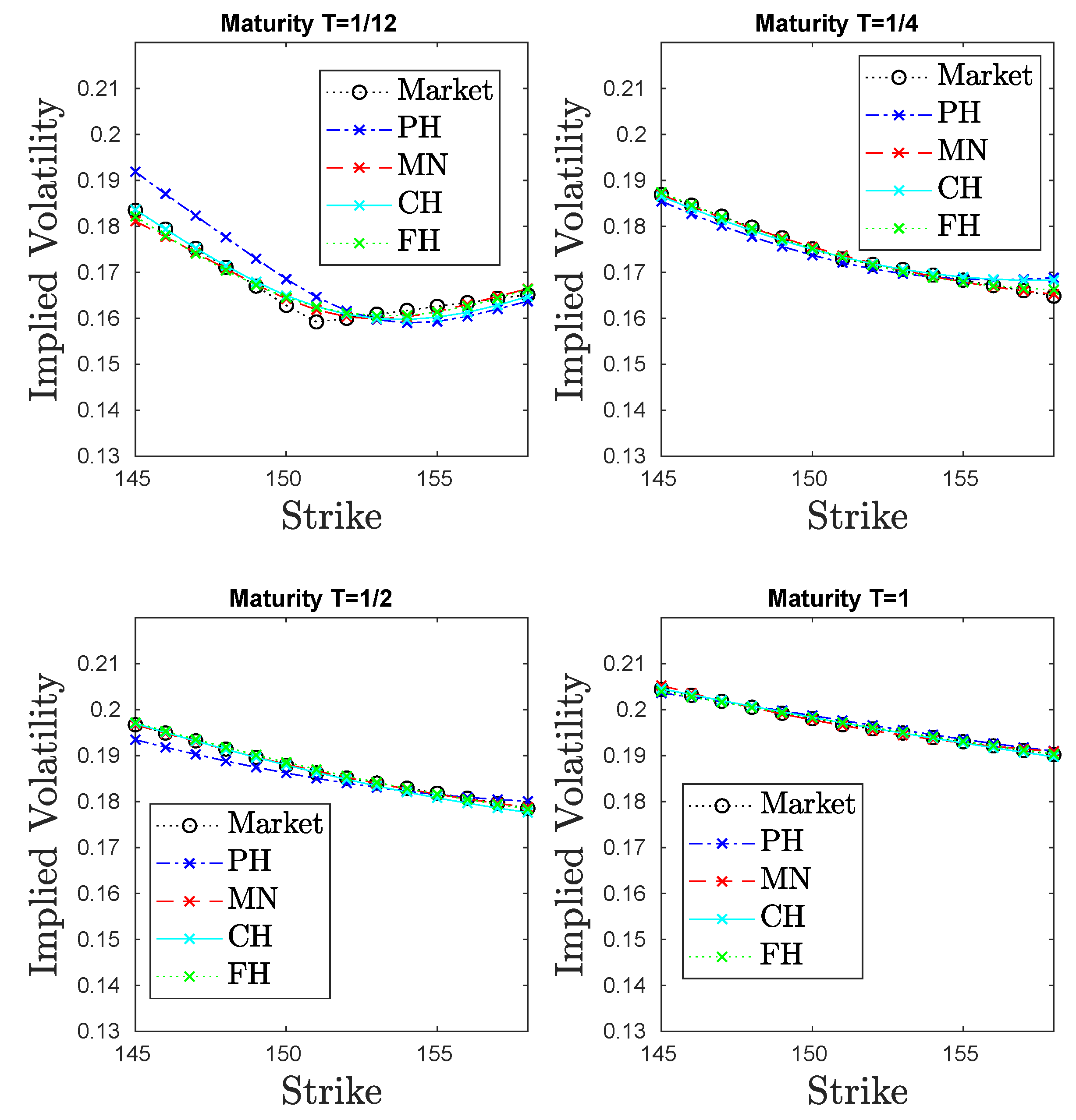
We observe that the estimation error with the FH model is clearly less than the errors with the PH, CH, and MN (sum of errors for each maturity) models. Furthermore, in Figure 1, we display and compare the implied volatilities for all of the models to the market volatilities for a clear illustration.

One see that the implied volatilities for our new model (FH) are much closer to the market volatilities than that for the PH model, especially when that $T=1/12.$ Furthermore, the implied volatilities for our model are slightly better when compared with both the CH and MN models.

6. Conclusions

In this work, we proposed a new correlation flow that is driven by isospectral flow, which provides the valid time-dependent correlation matrix at each time instance. Furthermore, we showed that the proposed correlation flow can be easily incorporated into another financial model via the time-dependently correlated BMs. The included correlation flow allows us to choose, in a reasonable way, additional (arbitrarily many) parameters to increase the fitting quality. We incorporated our proposed correlation flow into the Heston model, and analyzed its numerical approximation using both the BSDE- and ODE-methods. For comparative purposes, we fit several different models to the same market data. The numerical calibration results show that the Heston model extended by using correlation flow provides better volatility smiles than the Heston model with other considered extensions. Our findings show, again, that a non-constant correlation should be used in practical applications, and the behavior of real market can thus be described better. Furthermore, note that the correlation flow can also be applied to some other financial models for pricing and hedging by replacing the constant correlation for a better performance, as market requires.