Modified Hybrid Method with Four Stages for Second Order Ordinary Differential Equations

Abstract

A modified explicit hybrid method with four stages is presented, with the first stage exactly integrating exp(wx), while the remaining stages exactly integrate sin(wx) and cos(wx). Special attention is paid to the phase properties of the method during the process of parameter selection. Numerical comparisons of the proposed and existing hybrid methods for several second-order problems show that the proposed method gives high accuracy in solving the Duffing equation and Kramarz’s system.

1. Introduction

Many problems that arise in modelling physical phenomena in engineering and applied sciences are in the form of second ordinary initial value problems

$$y^{″}(t)=f(t,y(t)),y(t_0)=y_0,y^{\prime }(t_0)={y^{\prime }}_0$$

where the first derivative does not appear explicitly. These problems are often solved by using numerical methods such as Runge–Kutta–Nystrom methods, multistep methods, and hybrid methods (see [1,2,3,4]). The numerical methods can be grouped into two categories: (1) methods with constant coefficients and (2) methods with variable coefficients. The methods with variable coefficients require prior knowledge of the frequency of the problem, in contrast to the methods with constant coefficients in which the frequency of the problem is not needed. In this paper, our purpose is to derive a modified hybrid method with variable coefficients for solving the special second-order initial value problems by paying special attention to the phase properties of the methods.

Consider the class of hybrid methods proposed by Kalogiratou et al. [5]:

$$y_{n+1}=2{\sigma }_{s+1}{y}_n-{\mu }_{s+1}{y}_{n-1}+h^2{\displaystyle \sum _{j=1}^s{b}_{j}f(t_n+c_{j}h,g_j)}$$

(1)

with $g_i={\sigma }_i(1+c_i)y_n-{\mu }_i{c}_i{y}_{n-1}+h^2{\displaystyle \sum _{j=1}^s{a}_{ij}f(t_n+c_{j}h,g_j)},\hspace{0.33em}i=1,\dots ,s.$ It is noted that if ${\sigma }_i=1$ and ${\mu }_i=1$ for i = 1, …, s + 1 then the above class of hybrid methods is reduced to the class of hybrid methods as stated in [6]:

$$y_{n+1}=2y_n-y_{n-1}+h^2{\displaystyle \sum _{j=1}^s{b}_{j}f(t_n+c_{j}h,g_j)}$$

(2)

with $g_i=(1+c_i)y_n-c_i{y}_{n-1}+h^2{\displaystyle \sum _{j=1}^s{a}_{ij}f(t_n+c_{j}h,g_j)}.$

Coefficients of this class of methods are as shown in Butcher tableau notation below:

$$\begin{array}{cc}c& A\\ & b^T\end{array}$$

with $c^T=(\begin{array}{cccc}{c}_1& c_2& \cdots & c_s\end{array})$, $b^T=(\begin{array}{cccc}{b}_1& b_2& \cdots & b_s\end{array})$, and $A={[a_{ij}]}_{s\times s}$.

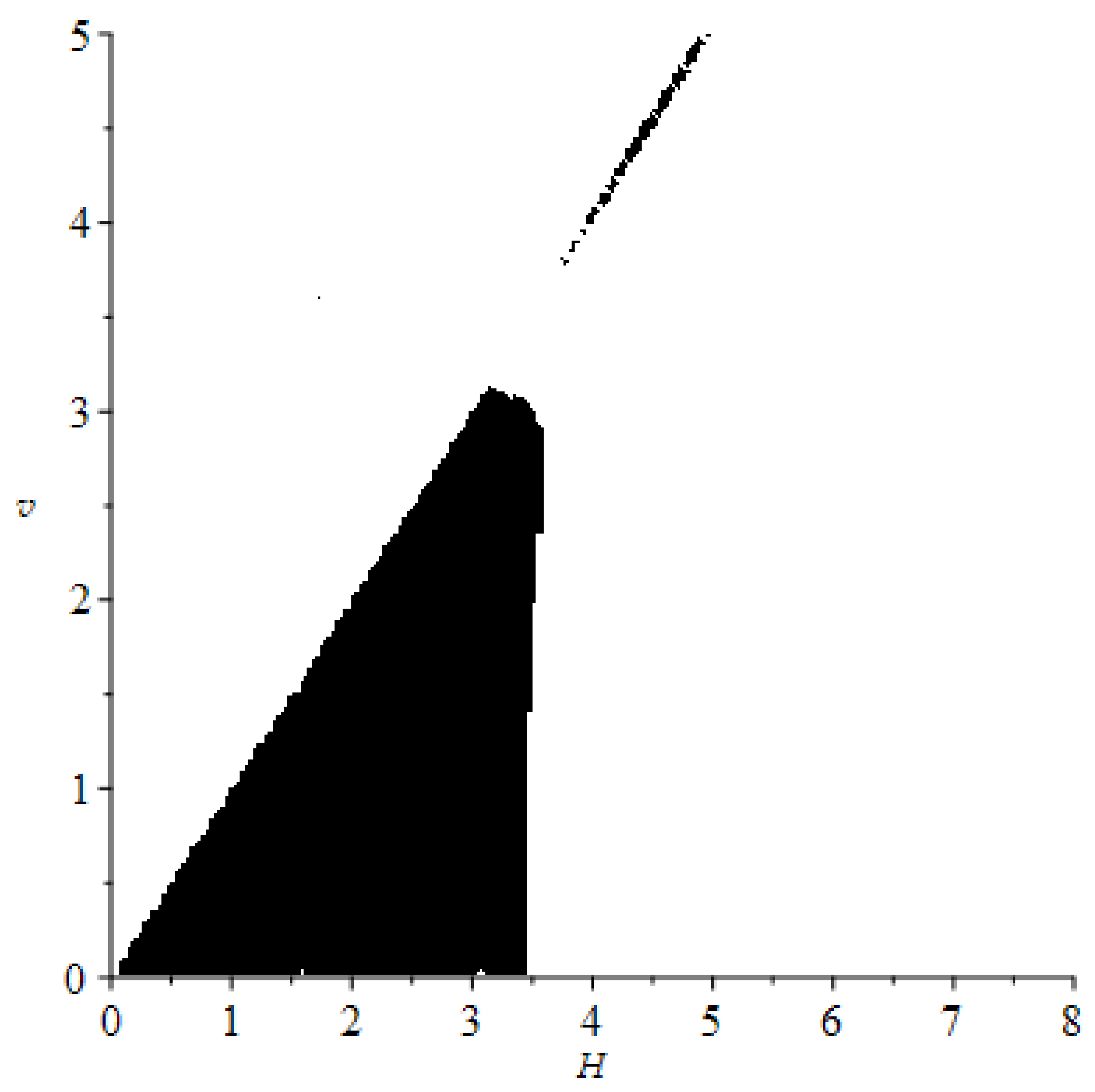
2. Phase Lag and Stability Analysis

The standard equation

$$y^{″}(t)=-{\lambda }^{2}y(t), \lambda >0$$

(3)

with exact solution $y(t)=C_1\exp (i\lambda t)+C_2\exp (-i\lambda t)$ is usually used to study the stability of numerical methods in solving second-order ordinary differential equations. Applying the hybrid methods defined in (1) with coefficients depending on v = wh, where w is the frequency of the problem and h is the step-size, to the differential Equation (3) gives us

$$y_{n+1}-S(H^2,v)y_n+P(H^2,v)y_{n-1}=0$$

(4)

where H = λh, $e=(\begin{array}{cccc}1& 1& \cdots & 1{)}^T\end{array}$, $\sigma (v)=(\begin{array}{cccc}{\sigma }_1& {\sigma }_2& \cdots & {\sigma }_s{)}^T\end{array}$, $\mu (v)={(\begin{array}{cccc}{\mu }_1& {\mu }_2& \cdots & {\mu }_s\end{array})}^T$, $S(H^2,v)=2{\sigma }_{s+1}-H^2{b}^T{(I+H^{2}A)}^{-1}\sigma (v)\times (e+c)$, $P(H^2,v)={\mu }_{s+1}-H^2{b}^T{(I+H^{2}A)}^{-1}\mu (v)\times c$ and the symbol “×” denotes component-wise multiplication. The characteristic polynomial associated with the difference Equation (4) is given by

$$\pi (\varsigma )={\varsigma }^2-S(H^2,v)\varsigma +P(H^2,v)$$

(5)

The following definition gives a condition to be satisfied by the region of absolute stability of hybrid methods (refer to [5]).

Definition 1.

For hybrid methods corresponding to Equation (5), a region of absolute stability is the region of the H-v plane throughout which$\left|P(H^2,v)\right|<1$and$\left|S(H^2,v)\right|<1+P(H^2,v)$.

The phase properties of hybrid methods are given by these definitions (refer to [7]).

Definition 2.

For hybrid methods corresponding to Equation (5), the phase-lag or dispersion error is given by$\varphi (H^2,v)=H-\arccos \left(S(H^2,v)/2\sqrt{P(H^2,v)}\right)$and the phase-lag order is q if$\varphi (H^2,v)=c_{\varphi }{H}^{q+1}+O(H^{q+3}).$

Definition 3.

For hybrid methods corresponding to Equation (5), the amplification or dissipation error is given by$d(H^2,v)=1-\sqrt{P(H^2,v)}$and the dissipation order is u if$d(H^2,v)=c_d{H}^{u+1}+O(H^{u+3})$. The method is called zero dissipative if$d(H^2,v)=0$

3. Derivation of the New Method

Consider the coefficients of a class of four-stage explicit hybrid methods defined in (1) as stated in

Table 1. Coefficients of a class of four-stage explicit hybrid methods defined in (1).

0	0	0	0	0	0	0
1	${\sigma }_2$	${\mu }_2$	$a_{21}$	0	0	0
$c_3$	${\sigma }_3$	${\mu }_3$	$a_{31}$	$a_{32}$	0	0
$c_4$	${\sigma }_4$	${\mu }_4$	$a_{41}$	$a_{42}$	$a_{43}$	0
	${\sigma }_5$	${\mu }_5$	$b_1$	$b_2$	$b_3$	$b_4$

.

Using these coefficients, $P(H^2,v)$ is given by

$$\begin{array}{l}P(H^2,v)=-H^2{\mu }_2((H^2{a}_{43})b_4-b_3)(H^2{a}_{32})+H^2(H^2{a}_{43})b_4{c}_3{\mu }_3+H^2(H^2{a}_{42})b_4{\mu }_2+\\ (-b_3{c}_3{\mu }_3-b_4{c}_4{\mu }_4-b_2{\mu }_2)H^2+{\mu }_5\end{array}$$

Setting $b_1=0$, $a_{32}=0$, $a_{42}=0$, and $a_{43}=0$, then solving the order conditions for fourth-order hybrid method as listed in [6]

$$\begin{array}{l}{b}_1+b_2+b_3+b_4=1\\ b_2+b_3{c}_3+b_4{c}_4=0\\ b_2+b_3{c}_3^2+b_4{c}_4^2=\frac{1}{6}\\ b_2{a}_{21}+b_3{a}_{31}+b_3{a}_{32}+b_4{a}_{41}+b_4{a}_{42}+b_4{a}_{43}=\frac{1}{12}\\ b_2+b_3{c}_3^3+b_4{c}_4^3=0\\ b_2{a}_{21}+b_3{c}_3{a}_{31}+b_3{c}_3{a}_{32}+b_4{c}_4{a}_{41}+b_4{c}_4{a}_{42}+b_4{c}_4{a}_{43}=\frac{1}{12}\\ b_3{a}_{32}+b_4{a}_{42}+b_4{a}_{43}{c}_3=0\end{array}$$

yields

$$b_2=\frac{6c_4^2-1}{6(-1+c_4)(7c_4+2)},b_3=\frac{216c_4^3+108c_4^2+18c_4+1}{6(7c_4+2)(6c_4^2+2c_4+1)}, b_4=-\frac{5}{6(-1+c_4)(6c_4^2+2c_4+1)}$$

$$a_{31}=\frac{-2-5c_4+7c_4^2+a_{21}(2-12c_4^2)}{2{(1+6c_4)}^2},$$

$$a_{4}1=-\frac{7}{10}{c}_4^2+\frac{6}{5}{c}_4^2{a}_{21}+\frac{1}{2}{c}_4+\frac{1}{5}-\frac{1}{5}{a}_{21},$$

$$c_3=-\frac{c_4+1}{1+6c_4}$$

where $c_4$ and $a_{21}$ are free parameters. By experiment, we choose $c_4=-\frac{1}{2}$ to make $P(H^2,v)$ as close as possible to 1 as $v\to 0$. In order to obtain $a_{21}$, ${\sigma }_i$ and ${\mu }_i$, we associate each stage formula of the method with linear operator $L\left[y(t)\right]$ as follows:

$$\begin{gathered} L_1\left[y(t)\right]=y(t+h)-2{\sigma }_{2}y(t)+{\mu }_{2}y(t-h)-h^2{a}_{21}{y}^{″}(t) \\ {L}_2\left[y(t)\right]=y(t+c_{3}h)-{\sigma }_3(1+c_3)y(t)+{\mu }_3{c}_{3}y(t-h)-h^2(a_{31}{y}^{″}(t)+a_{32}{y}^{″}(t+h)) \\ {L}_3\left[y(t)\right]=y(t+c_{4}h)-{\sigma }_4(1+c_4)y(t)+{\mu }_4{c}_{4}y(t-h)-h^2(a_{41}{y}^{″}(t)+a_{42}{y}^{″}(t+h)+a_{43}{y}^{″}(t+c_{3}h)) \\ {L}_4\left[y(t)\right]=y(t+h)-2{\sigma }_{5}y(t)+{\mu }_{5}y(t-h)-h^2(b_1{y}^{″}(t)+b_2{y}^{″}(t+h)+b_3{y}^{″}(t+c_{3}h)+b_4{y}^{″}(t+c_{4}h)) \end{gathered}$$

Assume that v = wh. Setting $L_1\left[e^{wx}\right]=0$, $L_1\left[\sin (wx)\right]=0$ and $L_1\left[\cos (wx)\right]=0$ results in

$$a_{21}=\frac{e^{2v}-2e^v+1}{e^v{v}^2},{\sigma }_2=\frac{e^{2v}+2\cos (v)e^v-2e^v+1}{2e^v}, {\mu }_2=1$$

This implies $a_{31}=\frac{-(e^{2v}-2e^v+1)}{8e^v{v}^2}+\frac{9}{32}$ and $a_{41}=-\frac{9}{40}+\frac{e^{2v}-2e^v+1}{10e^v{v}^2}$. Finally, by setting

$$L_2\left[\sin (wx)\right]=0, L_2\left[\cos (wx)\right]=0, L_3\left[\sin (wx)\right]=0, L_3\left[\cos (wx)\right]=0, L_4\left[\sin (wx)\right]=0, \mathrm{and} L_4\left[\cos (wx)\right]=0$$

we have

$${\sigma }_3=\frac{1}{40\sin (v)e^v}(9e^v{v}^2\sin (v)+32\cos (v/4)\sin (v)e^v+32\sin (v/4)\cos (v)e^v-4\sin (v)e^{2v}+8\sin (v)e^v-4\sin (v))$$

$${\sigma }_4=\frac{1}{20\sin (v)e^v}(-9e^v{v}^2\sin (v)+40\cos (v/2)\sin (v)e^v-40\sin (v/2)\cos (v)e^v+4\sin (v)e^{2v}-8\sin (v)e^v+4\sin (v))$$

$$\begin{array}{l}{\sigma }_5=\frac{1}{27\sin (v)}(\cos (v)\sin (v)v^2+8\cos (v)\sin (v/4)v^2-5\cos (v)\sin (v/2)v^2+8\sin (v)\cos (v/4)v^2+\\ 5\sin (v)\cos (v/2)v^2+27\cos (v)\sin (v))\end{array}$$

$${\mu }_3=\frac{4\sin (v/4)}{\sin (v)}, {\mu }_4=\frac{2\sin (v/2)}{\sin (v)},$$

$${\mu }_5=\frac{1}{27\sin (v)}(v^2\sin (v)+16v^2\sin (v/4)-10v^2\sin (v/2)+27\sin (v))$$

The resulting method is denoted by MEHM. This method has the following quantities:

$$P(H^2,v)=\frac{(-2H^2+2v^2+54){\cos }^3(v/4)+(6H^2-6v^2-27)\cos (v/4)-4H^2+4v^2}{54{\cos }^3(v/4)-27\cos (v/4)}$$

$$\begin{array}{l}S(H^2,v)=\frac{1}{108(2{\cos }^3(v/4)-\cos (v/4))}(128{\cos }^7(v/4)v^2+3456{\cos }^7(v/4)-192{\cos }^5(v/4)v^2+256{\cos }^4(v/4)v^2\\ -5184co{s}^5(v/4)+80{\cos }^3(v/4)v^2-192{\cos }^2(v/4)v^2+2160{\cos }^3(v/4)+12\cos (v/4)v^2+16v^2-216\cos (v/4)+\\ (-128{\cos }^7(v/4)+192{\cos }^5(v/4)-18{\cos }^3(v/4)v^2-256{\cos }^4(v/4)-80{\cos }^3(v/4)+9\cos (v/4)v^2+\\ 192{\cos }^2(v/4)-12\cos (v/4)-16)H^2+(18{\cos }^3(v/4)-9\cos (v/4))H^4)\end{array}$$

It is also noted that $\underset{v\to 0}{\lim }P(H^2,v)=1$ and $\underset{v\to 0}{\lim }S(H^2,v)=-H^2+\frac{1}{12}{H}^4+2$, with $\frac{S(H^2,v)}{2}$ being the rational approximation for the cosine as v → 0. The method is considered to be zero dissipative whenever v → 0. Solving $-H^2+\frac{1}{12}{H}^4+2<2$ for H > 0, we obtain $H<2\sqrt{3}$. It is also observed that the local truncation error is O(h⁶) as v → 0. The region of absolute stability of this method depicted using Maple 2020 software is shown below in Figure 1.

4. Results

The new and existing codes are abbreviated as follows.

MEHM: The modified explicit hybrid method with four stages derived in this paper.

EHM5IIPA: The phase-fitted and amplification-fitted explicit hybrid method with four stages derived in [8]. This method was derived based on the fifth-order hybrid method of the form (2).

Several problems are used to provide numerical comparisons in a constant step-size setting. Maximum global errors produced by each method are tabulated in

Table 2. Maximum global error in solving Problem 1.

Step-Size	MEHM	EHM5IIPA
0.4	8.12463 × 10−6	3.03912 × 10−5
0.2	4.72859 × 10−7	1.19831 × 10−6
0.1	2.80407 × 10−8	4.23368 × 10−8
0.05	1.69979 × 10−9	1.41116 × 10−9
0.025	1.04445 × 10−10	4.55621 × 10−11

,

Table 3. Maximum global error in solving Problem 2.

Step-Size	MEHM	EHM5IIPA
0.4	2.48225 × 10−14	1.02736
0.2	5.51845 × 10−13	2.71483 × 10−1
0.1	2.95522 × 10−13	8.20955 × 10−2
0.05	3.76672 × 10−12	2.97346 × 10−3
0.025	4.66915 × 10−12	9.77418 × 10−5

,

Table 4. Maximum global error in solving Problem 3.

Step-Size	MEHM	EHM5IIPA
0.4	1.42361 × 10−2	2.29762 × 10−1
0.2	9.29187 × 10−4	1.98607 × 10−3
0.1	6.00156 × 10−5	1.82083 × 10−4
0.05	3.81442 × 10−6	6.89947 × 10−6
0.025	2.40430 × 10−7	2.27004 × 10−7

and

Table 5. Maximum global error in solving Problem 4.

Step-Size	MEHM	EHM5IIPA
0.05	1.16031 × 10−16	1.74602 × 10−16
0.025	1.72165 × 10−16	1.67037 × 10−15
0.0125	5.41637 × 10−15	5.97021 × 10−16
0.00625	7.41002 × 10−15	1.49427 × 10−14
0.003125	2.45548 × 10−14	5.03433 × 10−14

. All numerical computations have been done in Maple 2020 software with 20 precision digits.

• Problem 1 (Prothero–Robinson problem)

Source: D’Ambrosio et al. [9]

$$y^{″}(t)=-(y(t)-e^{-\mu t}))+{\mu }^2{e}^{(-\mu t)},\hspace{0.33em}y(0)=1,y^{\prime }(0)=-\mu ,\hspace{0.33em}0\le t\le 10$$

Exact solution: $y(t)=e^{-\mu t}$. We use v = h in computing the numerical solutions for μ = 1, with MEHM and EHM5IIPA codes.

• Problem 2 (Duffing equation)

Source: Yusufoğlu [10]

$$y^{″}(t)+3y(t)-2y^3(t)=\cos (t)\sin (2t),\hspace{0.33em}y(0)=0,\hspace{0.33em}{y}^{\prime }(0)=1,\hspace{0.33em}0\le t\le 20$$

Exact solution:$y(t)=\sin (t)$. For MEHM and EHM5IIPA codes, v = h was used.

• Problem 3 (The well-known two-body problem)

Source: Franco [11]

$$\begin{gathered} y_1^{″}=-\frac{y_1}{{(y_1^2+y_2^2)}^{(3/2)}},\hspace{0.33em}{y}_1(0)=1-e,y_1^{\prime }(0)=0, \\ {y}_2^{″}=-\frac{y_2}{{(y_1^2+y_2^2)}^{(3/2)}},\hspace{0.33em}{y}_2(0)=0,\hspace{0.33em}{y}_2^{\prime }(0)=\sqrt{\frac{1+e}{1-e}},\hspace{0.33em}0\le t\le 20 \end{gathered}$$

Exact solution:$y_1(t)=\cos (R)-e,\hspace{0.33em}{y}_2(t)=\sqrt{1-e^2}\sin (R)$, where R satisfies the Kepler’s equation $t=R-e\sin (R)$ and e is the eccentricity of the orbit. In this numerical experiment, we consider the case e = 0.03. For MEHM and EHM5IIPA codes, v = h.

• Problem 4 (Kramarz’s system)

Source: D’Ambrosio et al. [12]

$$y^{″}(t)=\left(\begin{array}{cc}\mu -2& 2\mu -2\\ 1-\mu & 1-2\mu \end{array}\right)y(t),\hspace{0.33em}y(0)=\left(\begin{array}{c}2\\ -1\end{array}\right),\hspace{0.33em}{y}^{\prime }(0)=\left(\begin{array}{c}0\\ 0\end{array}\right)$$

where $\mu =2500$ and $0\le t\le 5$.

Exact solution: $y_1(t)=2\cos (t),\hspace{0.33em}{y}_2(t)=-\cos (t).$ For both codes, v = h is used.

5. Discussion and Conclusions

In this paper, a modified explicit hybrid method with four stages was proposed. The derivation of the method is based on the modified formula of hybrid method given in (1) while taking into consideration $\underset{v\to 0}{\lim }P(H^2,v)$. For this method, it was our intention to achieve $\underset{v\to 0}{\lim }P(H^2,v)=1$ in such a way that $\frac{S(H^2,v)}{2}$ is the rational approximation for the cosine, as studied by Coleman [13]. Moreover, the first stage of the modified formula is imposed to exactly integrate $e^{wx}$, while the remaining stages are imposed to exactly integrate sin(wx) and cos(wx) where w ∈ C. The maximum global errors of the new method were tabulated and compared with that of the phase-fitted and amplification fi-ted hybrid method in [8]. From the numerical results, the new method was observed to achieve high accuracy in solving the Duffing equation and Kramarz’s system. Furthermore, the new method performs with better accuracy for bigger step-sizes than that of the existing method for solving both the Prothero and Robinson and the two-body problems. Hence, this study offers evidence that, by taking into account $\underset{v\to 0}{\lim }P(H^2,v)$, the resulting modified explicit hybrid method is capable of solving second-order ordinary differential equations $y^{″}(t)=f(t,y)$.

References

1. Simos, T.E.; Williams, P.S. New insights in the development of Numerov-type methods with minimal phase-lag for the numerical solution of the Schrodinger equation. Comput. Chem. 2001, 25, 77–82. [Google Scholar] [CrossRef]
2. Simos, T.E.; Dimas, E.; Sideridis, A.B. A Runge-Kutta-Nystrom method for the numerical integration of special second-order periodic initial-value problem. J. Comput. Appl. Math 1994, 51, 317–326. [Google Scholar] [CrossRef] [Green Version]
3. Li, J.; Wang, X. Multi-step Runge–Kutta–Nyström methods for special second-order initial value problems. Appl. Numer. Math 2017, 113, 54–70. [Google Scholar] [CrossRef]
4. Li, J.; Lu, M.; Qi, X. Trigonometrically fitted multi-step hybrid methods for oscillatory special second-order initial value problems. Int. J. Comput. Math 2018, 95, 979–997. [Google Scholar] [CrossRef]
5. Kalogiratou, Z.; Monovasilis, T.; Ramos, H.; Simos, T.E. A new approach on the construction of trigonometrically fitted two step hybrid methods. J. Comput. Appl. Math 2016, 303, 146–155. [Google Scholar] [CrossRef]
6. Coleman, J.P. Order conditions for a class of two-step methods for y″ = f(x,y). IMA J. Numer. Anal. 2003, 23, 197–220. [Google Scholar] [CrossRef]
7. Van de Vyver, H. An explicit Numerov-type method for second-order differential equations with oscillating solutions. Comput. Math. Appl. 2007, 53, 1339–1348. [Google Scholar] [CrossRef] [Green Version]
8. Samat, F.; Ismail, F.; Suleiman, M. Phase fitted and amplification fitted hybrid methods for solving second-order ordinary differential equations. IAENG Int. J. Appl. Math. 2013, 43, 99–105. [Google Scholar]
9. D’Ambrosio, R.; Paternoster, B.; Santomauro, G. Revised exponentially fitted Runge-Kutta-Nystrom methods. Appl. Math. Lett. 2014, 30, 56–60. [Google Scholar] [CrossRef]
10. Yusufoğlu, E. Numerical solution of Duffing equation by the Laplace decomposition algorithm. Appl. Math. Comput. 2006, 177, 572–580. [Google Scholar]
11. Franco, J.M. A class of explicit two-step hybrid methods for second-order IVPs. J. Comput. Appl. Math 2006, 187, 41–57. [Google Scholar] [CrossRef] [Green Version]
12. D’ Ambrosio, R.; Ferro, M.; Paternoster, B. Two step hybrid collocation methods for y″ = f(x,y). Appl. Math. Lett. 2009, 22, 1076–1080. [Google Scholar] [CrossRef] [Green Version]
13. Coleman, J.P. Numerical methods for y″ = f(x,y) via rational approximations for the cosine. IMA J. Numer. Anal. 1989, 9, 145–165. [Google Scholar] [CrossRef]
Figure 1. Region of absolute stability of the proposed method.
Mathematics 09 01028 g001