Modification of Newton-Househölder Method for Determining Multiple Roots of Unknown Multiplicity of Nonlinear Equations

Abstract

In this study, we propose an extension of the modified Newton-Househölder methods to find multiple roots with unknown multiplicity of nonlinear equations. With four functional evaluations per iteration, the proposed method achieves an optimal eighth order of convergence. The higher the convergence order, the quicker we get to the root with a high accuracy. The numerical examples have shown that this scheme can compete with the existing methods. This scheme is also stable across all of the functions tested based on the graphical basins of attraction.

1. Introduction

One of the most popular problems in mathematics has been finding roots of nonlinear equations $f\left(x\right)=0$. In practice, an exact solution to the root is almost impossible. And hence, an iterative scheme is necessary. The most famous method of finding a simple root iteratively is Newton’s method,

$$x_{n+1}=x_n-{\displaystyle \frac{f\left(x_n\right)}{f^{\prime }\left(x_n\right)}},$$

(1)

which converges quadratically provided the initial guess is sufficiently close to the real root. Since then, many researchers have improved the Newton method to higher orders of convergence (see [1,2,3,4,5]). An example of a method which has cubic convergence is Househölder’s method,

$$x_{n+1}=x_n-{\displaystyle \frac{f\left(x_n\right)}{f^{\prime }\left(x_n\right)}}-{\displaystyle \frac{f^2\left(x_n\right)f^{\prime \prime }\left(x_n\right)}{2f^{\prime 3}\left(x_n\right)}}.$$

(2)

Despite its high order of convergence, Househölder’s method (2) is not widely used because of the high number of function and derivative evaluations involved in the method. Some modified forms of Househölder’s methods are given in [6,7]. It is also hard for such methods to reach an optimal convergence order based on the Kung-Traub hypothesis [8], which states that an iterative scheme can reach the optimal convergence $2^k$ when the number of functional and the derivative evaluations is $k+1$.

The classical Newton method (1) will converge linearly to a multiple root [9]. The earliest modified version of (1) for approximating a multiple root is due to Schröder [10] and given as

$$x_{n+1}=x_n-m{\displaystyle \frac{f\left(x_n\right)}{f^{\prime }\left(x_n\right)}},$$

(3)

which converges quadratically, where m, the multiplicity of the root, needs to be known in advance. There have been quite a number of methods proposed for finding a multiple root of known multiplicity of nonlinear equations [11,12,13,14,15]. In practice, however, both the root and its multiplicty are unknown. Traub [16] converted the problem of approximating a multiple root of unknown multiplicity of $f\left(x\right)=0$ to finding a simple root of an equivalent problem via the transformation

$$\Phi \left(x\right)={\displaystyle \frac{f\left(x\right)}{f^{\prime }\left(x\right)}}.$$

(4)

However, in solving iteratively this transformed equation, evaluations of the first and second derivatives are required, which most of the time, are more complicated than the evaluation of f. Using a similar approach of Traub [16], Parida and Gupta [17] presented a scheme which works for both cases of roots with known and unknown multiplicity. By suitable accelerating generators of iterative functions, Petković et al. [18] proposed two classes of methods for both cases of roots with known and unknown multiplicity. A new fifth-order modified Newton’s method for finding multiple roots of nonlinear equations with unknown multiplicity was developed by Li et al. [19]. Sharma and Bahl [20] proposed a sixth-order modified Newton’s method based on Traub’s [16] transformation. Jaiswal [21] claimed to be the first to propose an optimal eighth-order method for multiple roots of unknown multiplicity. Many researchers have modified the Newton method using Schröder’s approach [10] to develop new optimal methods for finding multiple roots [11,12,13,14,22,23]. However, there have been much less work done on developing methods using Traub’s conceptual approach [16].

In this paper, we aim to modify a Newton-Househölder method by adopting Traub’s concept and approximating the weight function as a rational function. The optimal method we propose for finding multiple roots of unknown multiplicity is eighth-order with four functional evaluations at each iteration.

2. Development of the Methods and Convergence Analysis

The Househölder method only achieves convergence of order three and it is not optimal according to the Kung-Traub conjecture. By eliminating the second derivative, the Househölder method can be made optimal. A modified version of the three-step Newton-Househölder method for approximating a simple root has been proposed by Sariman and Hashim [24] recently. The method is optimal and of eight order. Our motivation here is to develop an optimal eighth-order Newton-Househölder method for finding a multiple root with unknown multiplicity.

We begin with the following family of Newton-Househölder method for a simple root:

$$\begin{array}{cc}\hfill y_n& =x_n-{\displaystyle \frac{f\left(x_n\right)}{f^{\prime }\left(x_n\right)}},\hfill \\ \hfill z_n& =y_n-{\displaystyle \frac{f\left(y_n\right)}{f^{\prime }\left(x_n\right)}}-{\displaystyle \frac{f{\left(y_n\right)}^2}{2f^{\prime 3}\left(x_n\right)}}\left({\displaystyle \frac{\alpha f\left(y_n\right)+\beta f\left(x_n\right)}{{(y_n-x_n)}^2}}\right),\hfill \\ \hfill x_{n+1}& =z_n-{\displaystyle \frac{f\left(z_n\right)}{f^{\prime }\left(z_n\right)}},\hfill \end{array}$$

(5)

where $\alpha ,\beta \in \mathbb{R}$. First, we approximate $f^{\prime }\left(z_n\right)$ by

$$f^{\prime }\left(z_n\right)\approx {\displaystyle \frac{f^{\prime }\left(x_n\right)}{\eta (s,u)}},$$

(6)

where $s=f\left(y_n\right)/f\left(x_n\right)$ and $u=f\left(z_n\right)/f\left(y_n\right)$. Next, following Lee et al. [25], we approximate $\eta (s,u)$ by the rational function

$$\eta (s,u)={\displaystyle \frac{p_0+p_{1}s+p_2{s}^2+p_3{s}^3+u(p_4+p_{5}s+p_6{s}^2)}{q_0+q_{1}s+q_2{s}^2+q_3{s}^3+u(q_4+q_{5}s+q_6{s}^2)}},$$

(7)

where $p_n,q_n(0\le n\le 6)\in \mathbb{R}$. Substituting (6) and (7) into (5), we get

$$\begin{array}{cc}\hfill y_n& =x_n-{\displaystyle \frac{f\left(x_n\right)}{f^{\prime }\left(x_n\right)}},\hfill \\ \hfill z_n& =y_n-{\displaystyle \frac{f\left(y_n\right)}{f^{\prime }\left(x_n\right)}}-{\displaystyle \frac{f{\left(y_n\right)}^2}{2f^{\prime 3}\left(x_n\right)}}\left({\displaystyle \frac{\alpha f\left(y_n\right)+\beta f\left(x_n\right)}{{(y_n-x_n)}^2}}\right),\hfill \\ \hfill x_{n+1}& =z_n-{\displaystyle \frac{f\left(z_n\right)}{f^{\prime }\left(x_n\right)}}\left({\displaystyle \frac{p_0+p_{1}s+p_2{s}^2+p_3{s}^3+u(p_4+p_{5}s+p_6{s}^2)}{q_0+q_{1}s+q_2{s}^2+q_3{s}^3+u(q_4+q_{5}s+q_6{s}^2)}}\right).\hfill \end{array}$$

(8)

To make (8) efficient for finding multiple roots, we adopt the idea that has been presented by Traub [16]. Hence, the new optimal method for multiple roots based on the Newton-Househölder scheme can be written as

$$\begin{array}{cc}\hfill y_n& =x_n-{\displaystyle \frac{\Phi \left(x_n\right)}{{\Phi }^{\prime }\left(x_n\right)}},\hfill \\ \hfill z_n& =y_n-{\displaystyle \frac{\Phi \left(y_n\right)}{{\Phi }^{\prime }\left(x_n\right)}}-{\displaystyle \frac{\Phi {\left(y_n\right)}^2}{2{\Phi }^{\prime 3}\left(x_n\right)}}\left({\displaystyle \frac{\alpha \Phi \left(y_n\right)+\beta \Phi \left(x_n\right)}{{(y_n-x_n)}^2}}\right),\hfill \\ \hfill x_{n+1}& =z_n-{\displaystyle \frac{\Phi \left(z_n\right)}{{\Phi }^{\prime }\left(x_n\right)}}\left({\displaystyle \frac{p_0+p_{1}s+p_2{s}^2+p_3{s}^3+u(p_4+p_{5}s+p_6{s}^2)}{q_0+q_{1}s+q_2{s}^2+q_3{s}^3+u(q_4+q_{5}s+q_6{s}^2)}}\right),\hfill \end{array}$$

(9)

where $\Phi \left(x\right)=f\left(x\right)/f^{\prime }\left(x\right)$, $s=\Phi \left(y_n\right)/\Phi \left(x_n\right)$, $u=\Phi \left(z_n\right)/\Phi \left(y_n\right)$ and $\alpha ,\beta ,p_n,q_n(0\le n\le 6)\in \mathbb{R}$. The scheme yields the optimal order of eight with four functional evaluations. The convergence proof of the scheme (9) is given next.

Theorem 1.

Assume that $\gamma \in \mathbb{C}$ is the root of $f\left(x\right)$ with multiplicity m. If the initial value $x_0$ is sufficiently close to the root γ, the iteration scheme (9) can reach a convergence order of eight when

$$\begin{array}{cc}\hfill \alpha =10,\beta =4,p_0=q_0=-8,p_2& =-16,p_3=25,q_1=16,q_3=-23,q_4=8,\hfill \\ \hfill p_1=p_4=p_5& =p_6=q_2=q_5=q_6=0,\hfill \end{array}$$

or

$$\begin{array}{cc}\hfill \alpha =10,\beta =4,p_0=q_0=1,p_1=p_6& =2,p_2=p_3=6,p_4=-1,q_4=-2,\hfill \\ \hfill p_5=q_1=q_2=& q_3=q_5=q_6=0.\hfill \end{array}$$

Proof. 

Let $f\left(x\right)$ be defined as

$$f\left(x\right)={(x-\gamma )}^{m}G\left(x\right),$$

(10)

where $\gamma$ is a multiple root of the function $f\left(x\right)$ with multiplicity m if $f\left(x\right)\ne 0$ and $G\left(\gamma \right)\ne 0$. The first-order derivative of $f\left(x\right)$ is

$$f^{\prime }\left(x\right)=m{(x-\gamma )}^{m-1}G\left(x\right)+{(x-\gamma )}^m{G}^{\prime }\left(x\right).$$

(11)

Substituting Equations (10) and (11) into Equation (4), we get a new kind of transformation function $\Phi \left(x\right)$,

$$\Phi \left(x\right)={\displaystyle \frac{f\left(x\right)}{f^{\prime }\left(x\right)}}={\displaystyle \frac{(x-\gamma )G\left(x\right)}{mG\left(x\right)+(x-\gamma )G^{\prime }\left(x\right)}}.$$

(12)

Applying the transformation (12) to the scheme (8) for a simple root, the scheme will be transformed to another scheme for multiple roots. Now expanding $G\left(x\right)$ using the Taylor series about $\gamma$, we have

$$G\left(x_n\right)=G\left(\gamma \right)[1+c_1{e}_n+c_2{e}_n^2+c_3{e}_n^3+c_4{e}_n^4+c_5{e}_n^5+c_6{e}_n^6+c_7{e}_n^7+c_8{e}_n^8+c_9{e}_n^9+O\left(e_n^{10}\right)],$$

(13)

where $c_k=G^{\left(k\right)}\left(\gamma \right)/k!G\left(\gamma \right)$, $k=1,2,3,\dots$ and $e_n=x_n-\gamma$. Using (13) and its derivative, (12) can be written as:

$$\begin{array}{cc}\hfill \Phi \left(x_n\right)& ={\displaystyle \frac{e_{n}G\left(x_n\right)}{mG\left(x_n\right)+e_n{G}^{\prime }\left(x_n\right)}}\hfill \\ \hfill & ={\omega }_1{e}_n+{\omega }_2{e}_n^2+{\omega }_3{e}_n^3+{\omega }_4{e}_n^4+{\omega }_5{e}_n^5+{\omega }_6{e}_n^6+{\omega }_7{e}_n^7+{\omega }_8{e}_n^8+O\left(e_n^9\right),\hfill \end{array}$$

(14)

where

$$\begin{array}{cccc}\hfill {\omega }_1& =\frac{1}{m},\hfill & & \\ \hfill {\omega }_2& =\frac{c_1}{m^2},\hfill & & \\ \hfill {\omega }_3& =\frac{\left(c_1^2(m+1)-2c_{2}m\right)}{m^3},\hfill & & \\ \hfill {\omega }_4& =\frac{\left(-3c_3{m}^2+c_1^3\left(-{(m+1)}^2\right)+c_2{c}_{1}m(3m+4)\right)}{m^4},\hfill & & \\ \hfill {\omega }_5& =\frac{1}{m^5}\left(-2c_2{c}_1^{2}m\left(2m^2+5m+3\right)+2c_3{c}_1{m}^2(2m+3)+2m^2\left(c_2^2(m+2)-2c_{4}m\right)+c_1^4{(m+1)}^3\right),\hfill & & \\ \hfill {\omega }_6& =\frac{1}{m^6}[m^3(c_2{c}_3(5m+12)-5c_{5}m)-c_3{c}_1^2{m}^2(5m^2+14m+9)+c_1{m}^2(c_{4}m(5m+8)-c_2^2(5m^2\hfill \\ & +16m+12\left)\right)+c_1^5(-{(m+1)}^4)+c_2{c}_1^{3}m{(m+1)}^2(5m+8)],\hfill & & \\ \hfill {\omega }_7& =\frac{1}{m^7}[m^3(-2c_2^3{(m+2)}^2+2c_4{c}_{2}m(3m+8)+3m(c_3^2(m+3)-2c_{6}m))+6c_3{c}_1^3{m}^2{(m+1)}^2(m+2)\hfill \\ & +3c_1^2{m}^2(m^2+3m+2)(c_2^2(3m+4)-2c_{4}m)-2c_1{m}^3(2c_2{c}_3(3m^2+11m+9)-c_{5}m(3m+5))\hfill \\ & +c_1^6{(m+1)}^5-2c_2{c}_1^{4}m{(m+1)}^3(3m+5)],\hfill & & \\ \hfill {\omega }_8& =\frac{1}{m^8}[-c_3{c}_1^4{m}^2{(m+1)}^3(7m+15)-c_1^3{m}^2{(m+1)}^2(2c_2^2(7m^2+24m+20)-c_{4}m(7m+16))\hfill \\ & +m^4(c_3{c}_2^2(-(7m^2+32m+36))+c_5{c}_{2}m(7m+20)+m(c_3{c}_4(7m+24)-7c_{7}m))+c_1^2{m}^3\hfill \\ & \times (m+1)(3c_2{c}_3(7m^2+27m+24)-c_{5}m(7m+15))+c_1{m}^3(-2c_4{c}_{2}m(7m^2+28m+24)\hfill \\ & +m(c_{6}m(7m+12)-c_3^2(7m^2+30m+27))+c_2^3{(m+2)}^2(7m+8))+c_1^7(-{(m+1)}^6)\hfill \\ & +c_2{c}_1^{5}m{(m+1)}^4(7m+12)].\hfill & \end{array}$$

Next, substituting (14) and its derivative

$${\Phi }^{\prime }\left(x_n\right)={\omega }_1+2{\omega }_2{e}_n+3{\omega }_3{e}_n^2+4{\omega }_4{e}_n^3+5{\omega }_5{e}_n^4+6{\omega }_6{e}_n^5+7{\omega }_7{e}_n^6+8{\omega }_8{e}_n^7+O\left(e_n^8\right),$$

(15)

into the first substep of iteration scheme (9) gives

$$y_n-\gamma ={\psi }_2{e}_n^2+{\psi }_3{e}_n^3+{\psi }_4{e}_n^4+{\psi }_5{e}_n^5+{\psi }_6{e}_n^6+{\psi }_7{e}_n^7+{\psi }_8{e}_n^8+O\left(e_n^9\right),$$

(16)

where

$$\begin{array}{cccc}\hfill {\psi }_2& =-\frac{c_1}{m},\hfill & & \\ \hfill {\psi }_3& =\frac{2\left(c_1^2-2c_2\right)}{m},\hfill & & \\ \hfill {\psi }_4& =\frac{\left(c_1^3(1-3m)+c_2{c}_1(9m-2)-9c_{3}m\right)}{m^2},\hfill & & \\ \hfill {\psi }_5& =\frac{2\left(2c_1^4(m-1)+c_2{c}_1^2(7-8m)+c_3{c}_1(8m-3)+4c_2^2(m-1)-8c_{4}m\right)}{m^2},\hfill & & \\ \hfill {\psi }_6& =\frac{1}{m^3}[c_1^5(-5(m-2)m-1)+c_2{c}_1^3(m(25m-47)+4)+c_3{c}_1^{2}m(33-25m)+c_1(c_2^2\left(\right(48\hfill \\ & -25m)m-4)+c_{4}m(25m-12))+m(c_2{c}_3(25m-42)-25c_{5}m)],\hfill & & \\ \hfill {\psi }_7& =\frac{1}{m^3}\left[2\right(c_2^3(-6m^2+20m-8)+c_1^6(m-3)(3m-1)-2c_2{c}_1^4(m(9m-29)+8)+6c_3{c}_1^3\hfill \\ & \times (m(3m-8)+1)+3c_1^2(c_2^2(m(9m-29)+8)+2c_{4}m(5-3m))+2c_1(c_{5}m(9m-5)\hfill \\ & -2c_2{c}_3(m(9m-26)+3))+2c_2{c}_{4}m(9m-20)+9m(c_3^2(m-3)-2c_{6}m)\left)\right],\hfill & & \\ \hfill {\psi }_8& =\frac{1}{m^4}[c_1^7(1-7m((m-5)m+3))+c_2{c}_1^5(m(m(49m-240)+137)-6)+c_3{c}_1^{4}m\left(\right(214\hfill \\ & -49m)m-81)+c_1^3(2c_2^2(m((239-49m)m-136)+6)+c_{4}m(m(49m-163)+24))\hfill \\ & +c_1^{2}m(3c_2{c}_3(m(49m-221)+84)+c_{5}m(95-49m))+c_1\left(c_2^3\right(m(m(49m-242)+156)\hfill \\ & -8)-2c_4{c}_{2}m(7m(7m-26)+24)+m(c_3^2((219-49m)m-36)+c_{6}m(49m-30)))\hfill \\ & -m(c_3{c}_2^2(m(49m-232)+132)+c_5{c}_{2}m(130-49m)+m(c_3{c}_4(204-49m)+49c_{7}m))].\hfill & \end{array}$$

Substituting Equations (14)–(16) into the second substep of iterative scheme (9), we obtain

$$\begin{array}{cc}\hfill z_n-y_n& =-\frac{(\beta -4)c_1^2}{2m^2}{e}_n^3+\frac{\left(c_1^3(\alpha -3\beta +2(2\beta -7)m+4)+4(7-2\beta )c_2{c}_{1}m\right)}{2m^3}{e}_n^4\hfill \\ \hfill & +\sum _{k=0}^3{\zeta }_k{e}_n^{k+5}+O\left(e_n^9\right),\hfill \end{array}$$

(17)

where ${\zeta }_k={\zeta }_k(\alpha ,\beta ,m,c_1,c_2,\dots ,c_8)$. To eliminate $e_n^3$, we take $\beta =4$ and this gives

$$z_n-y_n=\frac{\left(c_1^3(\alpha +2m-8)-4c_1{c}_{2}m\right)}{2m^3}{e}_n^4+\sum _{k=0}^3{\Omega }_k{e}_n^{k+4}+O\left(e_n^9\right),$$

(18)

where

$$\begin{array}{cccc}\hfill {\Omega }_0& =\frac{\left(-6c_3{c}_1{m}^2-8c_2^2{m}^2+c_1^4(2(\alpha -4)+m(-3\alpha -4m+24))+2c_2{c}_1^{2}m(3(\alpha -8)+7m)\right)}{m^4},\hfill & & \\ \hfill {\Omega }_1& =\frac{1}{2m^5}[-84c_2{c}_3{m}^3+3c_3{c}_1^2{m}^2(9\alpha +22m-70)+8c_1{m}^2(c_2^2(6\alpha +12m-49)-3c_{4}m)\hfill \\ & +c_1^5(9\alpha +20m^3+21(\alpha -8)m^2-32(\alpha -4)m-24)+c_2{c}_1^{3}m(64(\alpha -4)+m(-75\alpha \hfill \\ & -94m+602\left)\right)],\hfill & & \\ \hfill {\Omega }_2& =\frac{1}{m^6}\left[2\right(2c_1{m}^3(c_2{c}_3(-27\alpha -52m+216)+5c_{5}m)+m^3(-4c_2^3(4\alpha +5m-34)+40c_4{c}_{2}m\hfill \\ & +27c_3^{2}m)+c_3{c}_1^3{m}^2(m(39\alpha +48m-308)-36(\alpha -4))+c_1^2{m}^2\left(c_2^2\right(m(84\alpha +87m-682)\hfill \\ & -96(\alpha -4))-2c_{4}m(6\alpha +15m-46))+2c_1^6(-2\alpha +m(11\alpha +5m^3+7(\alpha -8)m^2\hfill \\ & -18(\alpha -4)m-28)+4)+c_2{c}_1^{4}m(-44\alpha +m(132(\alpha -4)+m(-69\alpha -58m+554))\hfill \\ & +112\left)\right)],\hfill & & \\ \hfill {\Omega }_3& =\frac{1}{2m^7}[4m^4(2c_3(c_2^2(54\alpha +58m-453)-51c_{4}m)-65c_2{c}_{5}m)+c_1^2{m}^3\left(c_2{c}_3\right(1728\alpha -17m\hfill \\ & \times (81\alpha +78m-650)-6900)+5c_{5}m(15\alpha +38(m-3)))+c_1{m}^3(-4c_2^3(-256\alpha +m\hfill \\ & \times (156\alpha +121m-1286)+1028)+8c_4{c}_{2}m(48\alpha +91m-380)+3m\left(c_3^2\right(81\alpha +146m\hfill \\ & -636)-20c_{6}m\left)\right)+c_3{c}_1^4{m}^2(6(67\alpha -176)+m(-1120\alpha +m(537\alpha +428m-4268)\hfill \\ & +4482\left)\right)+c_1^3{m}^2(2c_2^2(688\alpha +m(-1696\alpha +m(687\alpha +478m-5555)+6792)-1664)\hfill \\ & +c_{4}m(8(32\alpha -129)+m(-267\alpha -326m+2090)))+c_1^7(5(5\alpha -8)+2m(-90\alpha \hfill \\ & +m(239\alpha +m(-240\alpha +7m(9(\alpha -8)+5m)+961)-592)+168\left)\right)+c_2{c}_1^{5}m(360\alpha \hfill \\ & +m(-1778\alpha +m(2464\alpha +m(-777\alpha -480m+6236)-9866)+4384)-672\left)\right].\hfill \end{array}$$

Using (14)–(18), the functions s and u can be rewritten as

$$\begin{array}{cc}\hfill s& =-\frac{c_1}{m}{e}_n+\frac{e^2\left(c_1^2(2m-1)-4c_{2}m\right)}{m^2}{e}_n^2+\sum _{k=0}^4{\xi }_k{e}_n^{k+3}+O\left(e_n^8\right),\hfill \end{array}$$

(19)

$$\begin{array}{cc}\hfill u& =\frac{\left(4c_{2}m-c_1^2(\alpha +2m-8)\right)}{2m^2}{e}_n^2+\sum _{k=0}^5{\theta }_k{e}_n^{k+2}+O\left(e_n^7\right),\hfill \end{array}$$

(20)

where ${\xi }_k={\xi }_k(m,c_1,c_2,\cdots ,c_8)$ and ${\theta }_k={\theta }_k(m,c_1,c_2,\cdots ,c_8)$ respectively. Substituting (14)–(20) into the third substep of iteration scheme (9), we get the error with the convergence order of four,

$$e_{n+1}=\frac{\left(c_1^3(\alpha +2m-8)-4c_1{c}_{2}m\right)\left(p_o-q_0\right)}{2\left(m^3{q}_0\right)}{e}_n^4+\sum _{k=0}^4{\mu }_k{e}_n^{k+4}+O\left(e_n^9\right),$$

(21)

where ${\mu }_k={\mu }_k(m,c_1,c_2,\cdots ,c_8)$.

Our intention is to achieve optimal convergence order of eight, and so we choose the values of the constants of $\alpha ,p_n$ and $q_n(0\le n\le 6)$ as follows:

$$\begin{array}{cc}\hfill \alpha =10,p_0=q_0=-8,p_2& =-16,p_3=25,q_1=16,q_3=-23,q_4=8,\hfill \\ \hfill p_1=p_4& =p_5=p_6=q_2=q_5=q_6=0.\hfill \end{array}$$

(22)

This yields the error

$$e_{n+1}=\frac{1}{4m^7}\left[c_1^2(c_1^2(m+1)-2c_{2}m)(12c_3{m}^2+c_1^3(2m-3)(2m+7)-4c_2{c}_{1}m(3m+4))\right]e_n^8+O\left(e_n^9\right).$$

(23)

Another set of parameter values that gives convergence of order eight is

$$\begin{array}{cc}\hfill \alpha =10,p_0=q_0=1,p_1=p_6& =2,p_2=p_3=6,p_4=-1,q_4=-2,\hfill \\ \hfill p_5=q_1=q_2=& q_3=q_5=q_6=0,\hfill \end{array}$$

(24)

which gives

$$e_n+1=\frac{c_1\left(c_2\left(c_1^2-4c_2\right)+3c_1{c}_3\right)\left(c_1^2(m+1)-2c_{2}m\right)}{m^5}{e}_n^8+O\left(e_n^9\right).$$

(25)

Based on the errors given in (23) and (25), we can conclude and confirm that our method has order of convergence eight with four functional evaluations ($\Phi \left(x_n\right)$, ${\Phi }^{\prime }\left(x_n\right)$, $\Phi \left(y_n\right)$, $\Phi \left(z_n\right)$) at each iteration. □

Based on the two sets of parameter values as given in (22) and (24), we obtain the following schemes:

• Taking the parameter values (22) for the weight function $\eta (s,u)$ and choosing $\alpha =10$ and $\beta =4$ in the proposed scheme (9), we obtain a new modified Newton-Househölder scheme for multiple roots with unknown multiplicity:

  $$\begin{array}{cc}\hfill y_n& =x_n-{\displaystyle \frac{\Phi \left(x_n\right)}{{\Phi }^{\prime }\left(x_n\right)}},\hfill \\ \hfill z_n& =y_n-{\displaystyle \frac{\Phi \left(y_n\right)}{{\Phi }^{\prime }\left(x_n\right)}}-{\displaystyle \frac{\Phi {\left(y_n\right)}^2}{2{\Phi }^{\prime 3}\left(x_n\right)}}\left({\displaystyle \frac{10\Phi \left(y_n\right)+4\Phi \left(x_n\right)}{{(y_n-x_n)}^2}}\right),\hfill \\ \hfill x_{n+1}& =z_n-{\displaystyle \frac{\Phi \left(z_n\right)}{{\Phi }^{\prime }\left(x_n\right)}}\left({\displaystyle \frac{-8-16s^2+25s^3}{-8+16s-23s^3+8u}}\right),\hfill \end{array}$$

  (26)

  where $\Phi \left(x_n\right)=f\left(x_n\right)/f^{\prime }\left(x_n\right)$, $s=\Phi \left(y_n\right)/\Phi \left(x_n\right)$ and $u=\Phi \left(z_n\right)/\Phi \left(y_n\right)$.
• Similarly, the parameter values in (24), and $\alpha =10$ and $\beta =4$ yield a scheme with the first two steps exactly the same as in (26) and a slightly different last step as follows:

  $$\begin{array}{cc}\hfill x_{n+1}& =z_n-{\displaystyle \frac{\Phi \left(z_n\right)}{{\Phi }^{\prime }\left(x_n\right)}}\left({\displaystyle \frac{1+2s+6s^3+2s^2(3+u)-u}{1-2u}}\right).\hfill \end{array}$$

  (27)

3. Numerical Examples

In this section, our methods (26) and (27), abbreviated as mNH1 and mNH2 respectively, will be compared against the classical Newton method (1), the methods of Jaiswal [21] and Zafar et al. [23], abbreviated as NM, JM and ZM respectively, and given below:

• Jaiswal [21] introduced the scheme that achieves optimal convergence order eight as follows:

  $$\begin{array}{cc}\hfill y_n& =x_n-{\displaystyle \frac{f\left(x_n\right)}{g_1(x_n,z_n)}},\hfill \\ \hfill u_n& =y_n-{\displaystyle \frac{f\left(y_n\right)}{g_2(x_n,y_n,z_n)}},\hfill \\ \hfill x_{n+1}& =u_n-{\displaystyle \frac{f\left(u_n\right)}{g_3(x_n,y_n,z_n,u_n)}},\hfill \end{array}$$

  (28)

  where

  $$\begin{array}{cc}\hfill f^{\prime }\left(x_n\right)& \approx {\displaystyle \frac{f\left(z_n\right)-f\left(x_n\right)}{f\left(x_n\right)}}=g_1(x_n,z_n),\hfill \\ \hfill f^{\prime }\left(y_n\right)& \approx {\displaystyle \frac{f[x_n,y_n]f[y_n,z_n]}{f[x_n,z_n]}}=g_2(x_n,y_n,z_n),\hfill \\ \hfill f^{\prime }\left(u_n\right)& \approx b_2-b_1{b}_4=g_3(x_n,y_n,z_n,u_n),\hfill \end{array}$$

  and $z_n=x_n+f\left(x_n\right)$, $b_1=f\left(u_n\right)$, $b_4=(f[y_n,u_n,x_n]-f[y_n,u_n,z_n])/(f[y_n,z_n]-f[y_n,x_n])$, $b_3=f[y_n,u_n,z_n]+b_{4}f[y_n,z_n]$ and $b_2=f[y_n,u_n]-b_3(y_n-u_n)+f\left(y_n\right)b_4$. The divided differences appearing above have their usual definitions.
• The following iterative method presented by Zafar et al. [23] has optimal convergence order of eight with four functional evaluations and derivations:

  $$\begin{array}{cc}\hfill y_n& =x_n-m{\displaystyle \frac{f\left(x_n\right)}{f^{\prime }\left(x_n\right)}},\hfill \\ \hfill z_n& =y_n-m\left({\displaystyle \frac{1+8u_n+11u_n^2}{1+6u_n}}\right){\displaystyle \frac{f\left(x_n\right)}{f^{\prime }\left(x_n\right)}}{u}_n,\hfill \\ \hfill x_{n+1}& =z_n-m\left(1+t_n+{\displaystyle \frac{t_n^2}{2}}+u_n(2+4t_n+w_n)\right){\displaystyle \frac{f\left(x_n\right)}{f^{\prime }\left(x_n\right)}}{w}_n,\hfill \end{array}$$

  (29)

  where $u_n={\left[f\left(y_n\right)/f\left(x_n\right)\right]}^{1/m}$, $t_n={\left[f\left(z_n\right)/f\left(y_n\right)\right]}^{1/m}$ and $w_n={\left[f\left(z_n\right)/f\left(x_n\right)\right]}^{1/m}$. The iteration scheme (29) still requires to identify the multiplicity of the roots before it can be used.

For comparison purposes, let us consider the test functions [26]:

• $f_1\left(x\right)=x(x^2+1)(2e^{x^2+1}+x^2-1){cosh}^3(\pi x/2)$, $\mathrm{root}=i$, $m=5$, $x_0=1.3i$
• $f_2\left(x\right)={(x{e}^{x^2}-{sin}^2\left(x\right)+3cos\left(x\right)+5)}^4$, $\mathrm{root}=-1.207647827\dots$, $m=4$, $x_0=-1$
• $f_3\left(x\right)={({sin}^2\left(x\right)-x^2+1)}^2$, $\mathrm{root}=1.404491648\dots$, $m=2$, $x_0=2$
• $f_4\left(x\right)={(x^2-e^x-3x+2)}^5$, $\mathrm{root}=0.2575302854\dots$, $m=5$, $x_0=0$.

The criteria that we desire to analyze are absolute difference between two consecutive iterations, $|x_n-x_{n-1}|$, the residual error of the corresponding function, $\left|f\right(x_n\left)\right|$, CPU time processing, $\tau$, in milliseconds, asymptotic error constant, $\eta =|x_n-x_{n-1}|/|x_{n-1}-x_{n-2}{|}^{\mu }$, theoretical order of convergence, $\mu \in {\mathbb{Z}}^{+}$, and computational order convergence, $\rho$, in [27] as follows:

$$\rho \approx {\displaystyle \frac{ln\left(\right|x_{n+1}-x_n|/|x_n-x_{n-1}\left|\right)}{ln\left(\right|x_n-x_{n-1}|/|x_{n-1}-x_{n-2}\left|\right)}}.$$

(30)

All calculations were performed using Maple 18 mathematical software, which uses multi-precision arithmetic with 3000 significant digits. In the numerical results, we marked $X\times {10}^{(\pm Y)}$ as $X(\pm Y)$.

First, in

Table 1. Results of $|x_n-x_{n-1}|$.

		NM	JM	ZM	mNH1	mNH2
$f_1\left(x\right)$	$|x_2-x_1|$	$4.72(-2)$	$6.97(-6)$	$8.31(-8)$	$4.08(-8)$	$3.16(-6)$
	$|x_3-x_2|$	$3.79(-2)$	$1.56(-42)$	$2.56(-58)$	$3.57(-61)$	$1.45(-45)$
	$|x_4-x_3|$	$3.05(-2)$	$9.77(-366)$	$2.09(-462)$	$1.22(-485)$	$2.89(-360)$
$f_2\left(x\right)$	$|x_2-x_1|$	$4.22(-2)$	$3.96(-5)$	$2.07(-2)$	$2.15(-5)$	$1.06(-5)$
	$|x_3-x_2|$	$2.77(-2)$	$6.87(-34)$	$2.07(-2)$	$1.16(-36)$	$1.63(-40)$
	$|x_4-x_3|$	$1.90(-2)$	$5.62(-264)$	$2.07(-2)$	$8.30(-287)$	$5.04(-319)$
$f_3\left(x\right)$	$|x_2-x_1|$	$1.50(-1)$	$5.64(-4)$	$2.37(-3)$	$1.38(-4)$	$1.14(-4)$
	$|x_3-x_2|$	$9.46(-2)$	$1.21(-27)$	$1.07(-20)$	$1.66(-31)$	$6.48(-33)$
	$|x_4-x_3|$	$5.63(-2)$	$5.20(-217)$	$1.72(-159)$	$7.31(-247)$	$7.02(-259)$
$f_4\left(x\right)$	$|x_2-x_1|$	$4.06(-2)$	$6.23(-9)$	$3.04(-10)$	$1.67(-9)$	$1.74(-9)$
	$|x_3-x_2|$	$3.28(-2)$	$7.80(-70)$	$9.14(-20)$	$4.15(-75)$	$1.25(-74)$
	$|x_4-x_3|$	$2.65(-2)$	$4.70(-557)$	$5.78(-80)$	$6.10(-600)$	$9.08(-596)$

, we give absolute difference between two consecutive iterations, $|x_n-x_{n-1}|$. We observe that mNH1 and mNH2 yield the smallest errors for all the test functions, with the exception of mNH2 for $f_1$.

Table 2. Results of $\left|f\right(x_n\left)\right|$.

		NM	JM	ZM	mNH1	mNH2
$f_1\left(x\right)$	$\left|f\right(x_1\left)\right|$	$4.63(-2)$	$7.67(-25)$	$1.85(-34)$	$5.27(-36)$	$1.46(-26)$
	$\left|f\right(x_2\left)\right|$	$1.52(-2)$	$4.29(-208)$	$5.14(-287)$	$2.69(-301)$	$3.00(-223)$
	$\left|f\right(x_3\left)\right|$	$4.98(-3)$	$4.14(-1674)$	$1.85(-2307)$	$1.24(-2433)$	$9.44(-1797)$
$f_2\left(x\right)$	$\left|f\right(x_1\left)\right|$	$2.92(+1)$	$4.20(-13)$	$9.02(+5180)$	$3.65(-14)$	$2.13(-15)$
	$\left|f\right(x_2\left)\right|$	$8.54\left(0\right)$	$3.80(-128)$	$1.09(+5177)$	$3.09(-139)$	$1.19(-154)$
	$\left|f\right(x_3\left)\right|$	$2.56\left(0\right)$	$1.70(-1048)$	$1.32(+5173)$	$8.08(-1140)$	$1.10(-1268)$
$f_3\left(x\right)$	$\left|f\right(x_1\left)\right|$	$1.39\left(0\right)$	$1.96(-6)$	$3.49(-5)$	$1.18(-7)$	$8.00(-8)$
	$\left|f\right(x_2\left)\right|$	$4.01(-1)$	$8.96(-54)$	$7.00(-40)$	$1.70(-61)$	$2.58(-64)$
	$\left|f\right(x_3\left)\right|$	$1.12(-1)$	$1.67(-432)$	$1.83(-317)$	$3.29(-492)$	$3.04(-516)$
$f_4\left(x\right)$	$\left|f\right(x_1\left)\right|$	$3.30(-1)$	$7.23(-39)$	$2.01(-45)$	$9.95(-42)$	$1.23(-41)$
	$\left|f\right(x_2\left)\right|$	$1.09(-1)$	$2.22(-343)$	$4.91(-93)$	$9.49(-370)$	$2.38(-367)$
	$\left|f\right(x_3\left)\right|$	$3.58(-2)$	$1.76(-2779)$	$4.96(-394)$	$6.49(-2994)$	$4.76(-2973)$

shows that the corresponding function’s absolute value, $\left|f\right(x_n\left)\right|$, up to the third iteration. We can see that our method mNH1 outperformed all the methods NM, JM and ZM, with mNH2 as the second best in most cases. We note that the method ZM diverges when applied to $f_2$, in addition it needs the multiplicity to be known.

Table 3. Result of $\eta ,\rho$ and $\tau$.

		NM	JM	ZM	mNH1	mNH2
$f_1\left(x\right)$	$\eta$	$2.13(+1)$	$2.79(-1)$	$1.12(-1)$	$4.63(-2)$	$1.46(-1)$
	$\rho$	0.9851	8.0000	8.0000	8.0000	8.0000
	$\tau$	640.0	484.0	235.0	281.0	266.0
$f_2\left(x\right)$	$\eta$	$2.47(+1)$	$1.13(+2)$	$6.21(+11)$	$2.51(+1)$	$1.04\left(0\right)$
	$\rho$	0.8999	8.0000	1.0008	8.0000	8.0000
	$\tau$	547.0	281.0	235.0	172.0	172.0
$f_3\left(x\right)$	$\eta$	6.3(0)	$1.17(-1)$	$1.04(+1)$	$1.26\left(0\right)$	$2.27(-1)$
	$\rho$	1.1281	8.0001	8.0005	8.0000	8.0001
	$\tau$	453.0	188.0	109.0	125.0	140.0
$f_4\left(x\right)$	$\eta$	$2.46(+1)$	$3.43(-5)$	$1.19(+73)$	$6.92(-5)$	$1.49(-4)$
	$\rho$	1.0111	8.0000	6.3212	8.0000	8.0000
	$\tau$	125.0	47.0	312.0	47.0	47.0

shows the methods with a near zero value of the absolute asymptotic error $\eta$ are mNH1, mNH2, and JM. The closer the value of the asymptotic error $\eta$ to zero, the faster the method converges to the root. The CPU time processing $\tau$ for mNH1 and mNH2 are much less compared to the NM, ZM and JM methods.

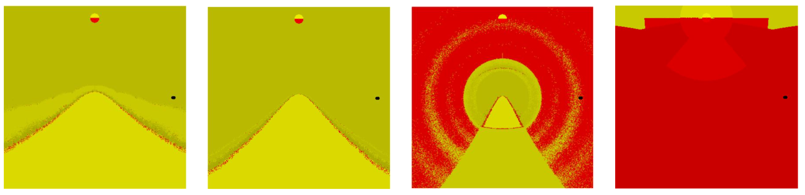
4. Basins of Attraction

In this section, we demonstrate the basins of attraction [28] to verify the stability of the proposed schemes. We present the basin of the attraction in the form of a rectangular image with dimensions $[-2,2]\times [-2,2]$ in $400\times 400$ grids. We run this analysis with a maximum of 100 iterations per point with the stopping convergence criterium set at ${10}^{-3}$. We note that a coloured region represents a convergence point, while the black region signifies a divergence point. For this purpose, we consider the test functions as given by Zafar et al. [23], Kumar et al. [29] and Alharbey et al. [30] (cf.

Table 4. Test functions for basins of attraction.

Function	Roots	Multiplicity
$g_1\left(z\right)=z^4+4z^3-24z^2+16z+16$	{$-7.4641,-0.535898,2,2$}	2
$g_2\left(z\right)={(z^3-1)}^2$	{$-0.5-0.866025i,-0.5-0.866025i,$	2
	$-0.5+0.866025i,-0.5+0.866025i,1,1$}
$g_3\left(z\right)=z^3-5.22z^2+9.0825z-5.2675$	{1.72,1.75,1.75}	2
$g_4\left(z\right)={(z^4-6z^2+8)}^2$	$\{-2,-2,-1.41421,-1.41421,$	2
	$1.41421,1.41421,2,2\}$

). Figure 1, Figure 2, Figure 3 and Figure 4 shows the images for the basins of attraction of each method. Figure 3, in particular, show that all the methods are convergent at all points for the function $g_3$. Overall, all the proposed methods have a stable scheme for finding the roots of nonlinear equations.

5. Conclusions

In this work, we have presented two optimal Newton-Househölder methods for finding multiple roots with unknown multiplicity of nonlinear equations. Convergence analysis was given to show that our methods are of eighth order. Such types of methods are desirable since, in practice, both the root and its multiplicity are unknown. In addition, our methods achieve a high order of convergence with four function evaluations per iteration. The effectiveness of the proposed methods has been demonstrated in terms of the CPU time speed, absolute error, and order of convergence. Furthermore, the schemes have been shown to be stable via the basins of attraction through several test functions. We conclude that our scheme can compete with other recent methods in finding multiple roots with unknown multiplicity of nonlinear equations. In our future work, we shall apply the CESTAC (Controle et Estimation Stochastique des Arrondis de Calculs) method [31] to obtain a new termination criterion instead of the traditional absolute error.

References

1. Geum, Y.H.; Kim, Y.I. A biparametric family of optimally convergent sixteenth-order multipoint methods with their fourth-step weighting function as a sum of a rational and a generic two-variable function. J. Comput. Appl. Math. 2011, 235, 3178–3188. [Google Scholar] [CrossRef] [Green Version]
2. Sharifi, S.; Salimi, M.; Siegmund, S.; Lotfi, T. A new class of optimal four-point methods with convergence order 16 for solving nonlinear equations. Math. Comput. Simul. 2016, 119, 69–90. [Google Scholar] [CrossRef] [Green Version]
3. Herceg, D.; Herceg, D. Eighth order family of iterative methods for nonlinear equations and their basins of attraction. J. Comput. Appl. Math. 2018, 343, 458–480. [Google Scholar] [CrossRef]
4. Junjua, M.u.D.; Zafar, F.; Yasmin, N. Optimal derivative-free root finding methods based on inverse interpolation. Mathematics 2019, 7, 164. [Google Scholar] [CrossRef] [Green Version]
5. Behl, R.; Salimi, M.; Ferrara, M.; Sharifi, S.; Alharbi, S.K. Some real-life applications of a newly constructed derivative free iterative scheme. Symmetry 2019, 11, 239. [Google Scholar] [CrossRef] [Green Version]
6. Noor, K.I.; Noor, M.A.; Momani, S. Modified Householder iterative method for nonlinear equations. Appl. Math. Comput. 2007, 190, 1534–1539. [Google Scholar] [CrossRef]
7. Tanveer, M.; Ahamd, M.; Ali, A.; Nazeer, W.; Rehman, K. Modified Householder’s method (MHHM) for solving nonlinear functions with convergence of order six. Sci. Int. 2016, 28, 83–87. [Google Scholar]
8. Kung, H.; Traub, J.F. Optimal order of one-point and multipoint iteration. J. ACM (JACM) 1974, 21, 643–651. [Google Scholar] [CrossRef]
9. Victory, H.D., Jr.; Neta, B. A higher order method for multiple zeros of nonlinear functions. Int. J. Comput. Math. 1983, 12, 329–335. [Google Scholar] [CrossRef]
10. Schröder, E. Über unendlich viele Algorithmen zur Auflösung der Gleichungen. Math. Ann. 1870, 2, 317–365. [Google Scholar] [CrossRef] [Green Version]
11. Geum, Y.H.; Kim, Y.I.; Neta, B. Constructing a family of optimal eighth-order modified Newton-type multiple-zero finders along with the dynamics behind their purely imaginary extraneous fixed points. J. Comput. Appl. Math. 2018, 333, 131–156. [Google Scholar] [CrossRef]
12. Sharma, J.R.; Kumar, S.; Jäntschi, L. On a class of optimal fourth order multiple root solvers without using derivatives. Symmetry 2019, 11, 1452. [Google Scholar] [CrossRef] [Green Version]
13. Alshomrani, A.S.; Behl, R.; Kanwar, V. An optimal reconstruction of Chebyshev–Halley type methods for nonlinear equations having multiple zeros. J. Comput. Appl. Math. 2019, 354, 651–662. [Google Scholar] [CrossRef]
14. Behl, R.; Argyros, I.K.; Argyros, M.; Salimi, M.; Alsolami, A.J. An iteration function having optimal eighth-order of convergence for multiple roots and local convergence. Mathematics 2020, 8, 1419. [Google Scholar] [CrossRef]
15. Alarcón, D.; Hueso, J.L.; Martínez, E. An alternative analysis for the local convergence of iterative methods for multiple roots including when the multiplicity is unknown. Int. J. Comput. Math. 2020, 97, 312–329. [Google Scholar] [CrossRef]
16. Traub, J. Iterative Methods for the Solution of Equations; Prentice Hall: Hoboken, NJ, USA, 1964. [Google Scholar]
17. Parida, P.K.; Gupta, D.K. An improved method for finding multiple roots and it’s multiplicity of nonlinear equations in IR. Appl. Math. Comput. 2008, 202, 498–503. [Google Scholar]
18. Petković, M.S.; Petković, L.D.; Džunić, J. Accelerating generators of iterative methods for finding multiple roots of nonlinear equations. Comput. Math. Appl. 2010, 59, 2784–2793. [Google Scholar] [CrossRef] [Green Version]
19. Li, X.; Mu, C.; Ma, J.; Hou, L. Fifth-order iterative method for finding multiple roots of nonlinear equations. Numer. Algorithms 2011, 57, 389–398. [Google Scholar] [CrossRef] [Green Version]
20. Sharma, R.; Bahl, A. A sixth order transformation method for finding multiple roots of nonlinear equations and basin attractors for various methods. Appl. Math. Comput. 2015, 269, 105–117. [Google Scholar] [CrossRef]
21. Jaiswal, J.P. An optimal order method for multiple roots in case of unknown multiplicity. Algorithms 2016, 9, 10. [Google Scholar] [CrossRef] [Green Version]
22. Behl, R.; Alsolami, A.J.; Pansera, B.A.; Al-Hamdan, W.M.; Salimi, M.; Ferrara, M. A new optimal family of Schröder’s method for multiple zeros. Mathematics 2019, 7, 1076. [Google Scholar] [CrossRef] [Green Version]
23. Zafar, F.; Cordero, A.; Junjua, M.u.D.; Torregrosa, J. Optimal eighth-order iterative methods for approximating multiple zeros of nonlinear functions. Rev. Real Acad. Cienc. Exactas Físicas Y Naturales. Ser. A. Matemáticas 2020, 114, 1–17. [Google Scholar] [CrossRef]
24. Sariman, S.A.; Hashim, I. New optimal Newton-Householder methods for solving nonlinear equations and their dynamics. CMC-Comput. Mater. Contin. 2020, 65, 69–85. [Google Scholar] [CrossRef]
25. Lee, S.D.; Kim, Y.I.; Neta, B. An optimal family of eighth-order simple-root finders with weight functions dependent on function-to-function ratios and their dynamics underlying extraneous fixed points. J. Comput. Appl. Math. 2017, 317, 31–54. [Google Scholar] [CrossRef]
26. Biazar, J.; Ghanbari, B. A new third-order family of nonlinear solvers for multiple roots. Comput. Math. Appl. 2010, 59, 3315–3319. [Google Scholar] [CrossRef] [Green Version]
27. Kumar, S.; Kumar, D.; Sharma, J.R.; Cesarano, C.; Agarwal, P.; Chu, Y.M. An optimal fourth order derivative-free numerical algorithm for multiple roots. Symmetry 2020, 12, 1038. [Google Scholar] [CrossRef]
28. Vrscay, E.R.; Gilbert, W.J. Extraneous fixed points, basin boundaries and chaotic dynamics for Schröder and König rational iteration functions. Numer. Math. 1987, 52, 1–16. [Google Scholar] [CrossRef]
29. Kumar, D.; Sharma, J.R.; Jăntschi, L. A novel family of efficient weighted-Newton multiple root iterations. Symmetry 2020, 12, 1494. [Google Scholar] [CrossRef]
30. Alharbey, R.A.; Kansal, M.; Behl, R.; Machado, J. Efficient three-step class of eighth-order multiple root solvers and their dynamics. Symmetry 2019, 11, 837. [Google Scholar] [CrossRef] [Green Version]
31. Noeiaghdam, S.; Araghi, M.A.F. Application of the CESTAC Method to Find the Optimal Iteration of the Homotopy Analysis Method for Solving Fuzzy Integral Equations. In International Online Conference on Intelligent Decision Science; Springer: Cham, Switzerland, 2020; pp. 623–637. [Google Scholar]
Figure 1. Basins of attraction of mNH1, mNH2, JM and ZM methods respectively for g 1 ( z ) .
Mathematics 09 01020 g001
Figure 2. Basins of attraction of mNH1, mNH2, JM and ZM methods respectively for g 2 ( z ) .
Mathematics 09 01020 g002
Figure 3. Basins of attraction of mNH1, mNH2, JM and ZM methods respectively for g 3 ( z ) .
Mathematics 09 01020 g003
Figure 4. Basins of attraction of mNH1, mNH2, JM and ZM methods repectively for g 4 ( z ) .
Mathematics 09 01020 g004