Unified Representation of Curves and Surfaces

Abstract

In conventional modeling, shared control points can be employed to realize a unified representation for an object consisting of only curves or only surfaces touching one another. However, this method fails in treating the following two cases: (a) a system consisting of detached curves or surfaces; (b) a system having both curves and surfaces. The purpose of the present paper is to develop a new theoretical tool to solve such problems. By introducing the definitions of naked knot and I-mesh, the concept of I-spline is put forth, which is, in essence, an expanded B-spline or T-spline. It is verified by examples that the naked knots make I-splines flexible and effective in transforming different surfaces and/or curves into a unified one, especially in the above two cases.

1. Introduction

In the computer-aided design of aircraft, cars, and ships, non-uniform rational B-splines (NURBS) are widely used in generating and representing curves and surfaces [1,2]. They have even been chosen by International Organization for Standardization (ISO) as the only mathematical tool to define the geometric shapes of industrial products. However, an obvious insufficiency of NURBS is that single NURBS can only represent the tensor product topology; thus, they are not so suitable for the local refinement of surfaces, due to their control points must form rectangular topologies and knot insertion will introduce at least one new row (column) of control points. In addition, the mesh of tensor product spline surface cannot contain extraordinary points, where the number of adjacent connected edges $n\ne 4$ [3]. To overcome those drawbacks, Sederberg et al. put forth T-splines [4,5], which have T-junctions in their control meshes and so can achieve flexible local refinement. Subsequently, research was done to complete the T-spline theory, including the linear independence of blending functions [6,7,8], local refinement algorithm [9,10,11,12], and other fundamental theories of T-splines [13,14,15]. It also extended the applications of NURBS and T-splines in CAD and CAE such as the isogeometric analysis [16] based integration of NURBS or T-splines with finite element analysis [17,18,19,20,21]. The unified representation in the isogeometric analysis may avoid the efficiency and accuracy problems caused by the transformation between the geometric design model and the analysis model.

Although B-splines and T-splines are effective in modeling a single curve or surface, they may encounter difficulties in representing complex objects. As is known, the body surface of a practical product usually has a large number of diverse curves and surfaces, which are represented separately by different B-splines in conventional modeling [1,2]. For example, the face-shaped curve model shown in Figure 1 is comprised of four curves that have different B-spline descriptions. This makes the whole representation very complex and the subsequent treatment troublesome. An effective way to reduce such complexity is to transform multiple curves or surfaces into a unified one. Generally, two curves or surfaces touching each other can be represented uniformly just by introducing shared control points. However, the unified representation cannot be generated in such a conventional way in the following two cases: (a) a system comprised of detached curves or surfaces (see Figure 1); (b) a system consisting of both curves and surfaces (see Figure 2).

The present paper aims at developing a new method for the unified representation of curves and/or surfaces in the abovementioned two cases. For this purpose, the definitions of naked knot and I-mesh are put forward at first, and then they are used to set up a unified representation-oriented concept of I-splines. The remainder of this paper is organized as follows. Section 2 reviews the concept of knot interval. Section 3 presents the theory of I-splines. To make the theory relatively complete, the local refinement is given in Section 4. Finally, the unified representation for the curves and/or surfaces in the abovementioned two cases is provided in Section 5 to demonstrate the effectiveness of the I-spline method, and some conclusions are drawn in Section 6.

2. Knot Interval

For the convenience of subsequent descriptions, the concept of knot interval is reviewed in this section. A knot interval means the distance between two adjacent knots in a knot vector [4], which is a non-negative value. Figure 3 shows a cubic B-spline curve and its topology, where the knot intervals and the control points are denoted by $d_i$ and $P_i$, respectively. In the cases of B-spline or T-spline surfaces, the edges of its control mesh can also be labeled by knot intervals [4]. In this way, the local knot coordinate system can then be set up for the description of curves and surfaces [4].

3. I-Splines

The concept of the I-spline is put forth in this section. For this purpose, the definitions of naked knot and I-mesh need to be given at first. Given the general expression of I-splines with an arbitrary degree is complicated, we only choose the cubic I-splines to make a demonstration here.

3.1. Basic Concepts

As is known, the topology of a B-spline curve is a straight line with several control points continuously distributed, and that of a B-spline surface is a planar orthotropic mesh with the control points located continuously in both parameters’ directions. As for a T-spline surface, its topology is also a planar orthotropic mesh, but there is a row or column of control points allowed to terminate, without traversing the entire topology. The junction at such a termination looks like the English letter “T”. Therefore, such meshes and splines are called T-meshes and T-splines, respectively. A common feature of the control-point distributions of B-splines and T-splines is that there is no naked knot among the control points. Here, the concept of the naked knot is introduced to denote a knot that has no coincident control point.

Such a lack of naked knots among control points restricts the flexibility of both B-splines and T-splines in some respects. For example, they cannot be employed to give a unified representation for a group of detached curves, or a group of surfaces and curves, as stated in Section 1. In this paper, such unified representations are achieved simply by inserting some naked knots among the control points of either B-splines or T-splines. After the insertion, the control points become discontinuous. In this case, the junction at a naked knot looks like the English letter “I”; so, we just call such meshes and the associated splines “I-meshes” and “I-splines”, respectively. Figure 4 illustrates the topologies of an I-spline curve and an I-spline surface, respectively. It is found that the control points become discontinuous due to the insertion of the naked knots (see the red control points therein). For an I-mesh, if two control points of a grid have the same value in one parameter, they must be connected.

Obviously, I-meshes are expanded B-meshes or T-meshes, and thus, the associated I-splines are expanded B-splines or T-splines. Therefore, the mathematical description of I-splines can be obtained by extending that of B-splines or T-splines as follows.

3.2. Mathematical Description

3.2.1. Coordinates of Control Points

To give the mathematical description for I-splines, one needs to determine the coordinates of control points at first. As in the cases of B-splines or T-splines, the coordinates of control points in an I-mesh can be determined by the knot intervals and the local knot coordinate system. Figure 5 shows the control points in both one-parameter and two-parameter topological spaces, respectively.

In principle, any control point can be taken as the coordinate origin for an I-mesh. Here, we just choose $P_1$ as the origin in Figure 5, and the horizontal and vertical knot lines penetrating it are then regarded as the axes. After the reference frame is set up, the knot intervals can then be employed to determine the coordinates of the control points. Nevertheless, it is not easy to give a general formula to calculate their coordinates directly, because there is an indefinite number of naked knots among the control points. Therefore, it is suggested to calculate the coordinates of the knots at first, and then to determine the coordinates of the control points according to their correspondence. Let $u_i$ be the coordinate of the ith knot in a one-dimensional topology. It can be found from Figure 5a that $u_i=u_{i-1}+d_i$, where $d_i$ is the corresponding knot interval. Let $(u_i,v_j)$ be the coordinate of the $(i,j)$ knot in a two-dimensional topology. Then, the coordinates of the knots in Figure 5b can be determined as $u_i=u_{i-1}+d_i$ and $v_j=v_{j-1}+e_j$, where $d_i$ and $e_j$ are the knot intervals in the horizontal and vertical directions, respectively. After the coordinates of the knots are determined, it is very easy to get those of the control points. For example, in Figure 5a, the knot coordinates for $P_1$ is $u_0$, for $P_2$ is $u_1=u_0+d_1$, for $P_3$ is $u_2=u_1+d_2$, and so on. In Figure 5b, the knot coordinates for $P_1$ are ($u_0$,$v_0$), and for $P_2$ are ($u_0+d_1+d_2+d_3$,$v_0$).

3.2.2. I-Spline Formula

Like in the cases of B-splines and T-splines, an I-spline defined in a $m$ dimensional topological space can be expressed by a function containing $m$ variables, i.e., $u_1$, $u_2$, $\cdots$, $u_m$, each of which corresponds to a specific dimension. For example, in the two-dimensional case shown in Figure 5b, the I-spline function only has two variables, $u$ and $v$. To construct a general formulation, $u$ and $v$ here are renamed as $u_1$ and $u_2$, respectively. In such a manner, one can formulate I-splines as follows

$$P\left(u_1,u_2\cdots ,u_m\right)={\displaystyle \sum _{i=1}^n{P}_i{B}_i\left(u_1,u_2\cdots ,u_m\right)}$$

(1)

where $P_i$ stands for the ith control point, and $B_i\left(u_1,u_2\cdots ,u_m\right)$ is the corresponding blending function given by

$$B_i\left(u_1,u_2\cdots ,u_m\right)={\displaystyle \prod _{j=1}^{m}N\left[u_{j,i}\right]\left(u_j\right)}$$

(2)

where $N\left[u_{j,i}\right]\left(u_j\right)$ is the jth basis function defined by the variable $u_j$ and the knot vector $u_{j,i}$. Here, the subscript $j$ stands for the jth dimension and $i$ represents the ith control point. In a one-dimensional topology (i.e., $m=1$), the knot vector $u_{1,i}$ is just written as $u_i$.

For a cubic I-spline in an m-dimensional topological space, the knot vector is

$$u_{j,i}=[u_{j,i-2}, u_{j,i-1}, u_{j,i}, u_{j,i+1}, u_{j,i+2}]$$

(3)

where $j=1, 2, \cdots , m$. For example, Figure 6a shows a cubic I-spline in a four-dimensional topological space. In this case, $j=1, 2, 3, 4$.

For a cubic I-spline in a one-dimensional topological space (see Figure 6b), the knot vector is given by

$$u_i=[u_{i-2}, u_{i-1}, u_i, u_{i+1}, u_{i+2}]$$

(4)

It is seen from the above equations that the formulas of I-splines have the same forms as those of B-splines or T-splines seemingly. However, it can be found from Figure 6 that naked knots exist among the control points of the I-mesh. But as is known, the B-spline or T-spline meshes do not have such naked knots. Therefore, this is the key difference, which will surely affect the values of knot vectors. It is also seen that I-splines can be applied to not only surfaces but also curves, and this expands the representation capability of conventional T-splines, which can only be used to generate surfaces generally. Next, detailed mathematical descriptions will be given to both I-spline curves and surfaces.

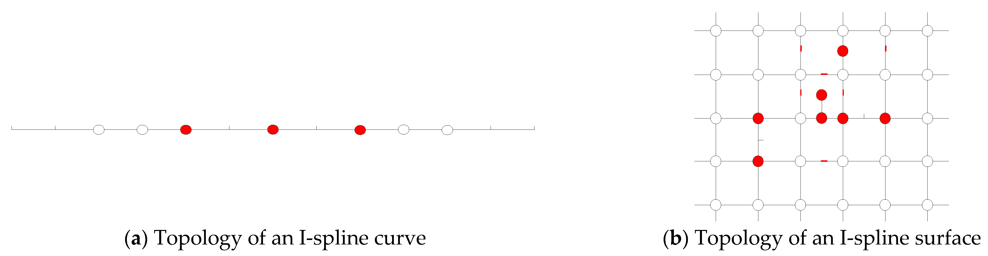
3.2.3. I-Spline Curves

Assume that $P_i=\left(w_i{x}_i,w_i{y}_i,w_i\right)$ is the ith control point of an I-spline curve and $w_i$ is the associated weight. Since the topology is a straight line, the I-spline curve can be formulated as the following one-variable function

$$P\left(u\right)=\frac{{\displaystyle \sum _{i=1}^n\left(x_i,y_i\right)B_i\left(u\right)}}{{\displaystyle \sum _{i=1}^n{w}_i{B}_i\left(u\right)}}$$

(5)

where $B_i(u)$ is the ith blending function given by

$$B_i\left(u\right)=N\left[u_i\right]\left(u\right).$$

(6)

where $N\left[u_i\right]\left(u\right)$ is the basis function, and $u_i$ is the knot vector, whose expression in cubic I-spline cases is shown in Equation (4).

3.2.4. I-Spline Surfaces

Consider an I-spline surface with its ith control point being $P_i=\left(w_i{x}_i,w_i{y}_i,w_i{z}_i,w_i\right)$. Since the surface has a two-dimensional topology, the I-spline formula takes the form of a two-variable function

$$P\left(u_1,u_2\right)=\frac{{\displaystyle \sum _{i=1}^n\left(x_i,y_i,z_i\right)B_i\left(u_1,u_2\right)}}{{\displaystyle \sum _{i=1}^n{w}_i{B}_i\left(u_1,u_2\right)}}$$

(7)

where $B_i(u_1,u_2)$ is the ith blending function defined by

$$B_i\left(u_1,u_2\right)=N\left[u_{1,i}\right]\left(u_1\right)N\left[u_{2,i}\right]\left(u_2\right)$$

(8)

In Equation (8), $N\left[u_{1,i}\right]\left(u_1\right)$ and $N\left[u_{2,i}\right]\left(u_2\right)$ are the basis functions; $u_{1,i}$ and $u_{2,i}$ are the knot vectors, whose expressions in cubic I-spline cases are

$$\begin{array}{l}{u}_{1,i}=[u_{1,i-2}, u_{1,i-1}, u_{1,i}, u_{1,i+1}, u_{1,i+2}]\\ u_{2,i}=[u_{2,i-2}, u_{2,i-1}, u_{2,i}, u_{2,i+1}, u_{2,i+2}]\end{array}\}$$

(9)

4. Local Refinement of I-Splines

The existence of naked knots makes I-splines locally refinable, and this is an advantage over conventional B-splines. This section presents the local refinement algorithm for I-splines, the key part of which is the refinement of the blending functions.

4.1. Refinement of the Blending Functions

Consider the blending function of cubic I-splines and the associated knot vector $u_{j,i}$. To refine the blending function, new knots need to be inserted into the knot vector. Although several knots can be inserted at the same time, only a single one is inserted here just for simplicity. In the cases of cubic I-splines, there are four intervals in every $u_{j,i}$ (see Equation (3)); thus, there are four different ways to perform the insertion. Since only cubic I-splines are considered here, two subsequences of the knot vector after insertion are used to construct the new blending functions. Then, the relations between the original and the new blending functions are given as follows.

Case 1: ${\overline{u}}_{j,i}=[u_{j,-2}, k, u_{j,-1}, u_{j,0}, u_{j,+1}, u_{j,+2}]$.

$$N[u_{j,i}](u_j)=\frac{k-u_{j,-2}}{u_{j,+1}-u_{j,-2}}N[{\tilde{u}}_{j,i}^{(1)}](u_j)+N[{\tilde{u}}_{j,i}^{(2)}](u_j)$$

(10)

where $N[{\tilde{u}}_{j,i}^{(1)}](u_j)$ and $N[{\tilde{u}}_{j,i}^{(2)}](u_j)$ are associated with the two subsequences ${\tilde{u}}_{j,i}^{(1)}=[u_{j,-2}, k, u_{j,-1}, u_{j,0}, u_{j,+1}]$ and ${\tilde{u}}_{j,i}^{(2)}=[k, u_{j,-1}, u_{j,0}, u_{j,+1}, u_{j,+2}]$, respectively.

The following relation can be obtained from Equation (10)

$$B_i=\frac{k-u_{j,-2}}{u_{j,+1}-u_{j,-2}}{\tilde{B}}_i^{(1)}+{\tilde{B}}_i^{(2)}$$

(11)

where the two new blending functions are ${\tilde{B}}_i^{(1)}=N[{\tilde{u}}_{j,i}^{(1)}](u_j){\displaystyle \prod _{c=1, c\ne j}^{m}N[u_{c,i}](u_c)}$ and ${\tilde{B}}_i^{(2)}=N[{\tilde{u}}_{j,i}^{(2)}](u_j){\displaystyle \prod _{c=1, c\ne j}^{m}N[u_{c,i}](u_c)}$.

Case 2: ${\overline{u}}_{j,i}=[u_{j,-2}, u_{j,-1}, k, u_{j,0}, u_{j,+1}, u_{j,+2}]$.

$$N[u_{j,i}](u_j)=\frac{k-u_{j,-2}}{u_{j,+1}-u_{j,-2}}N[{\tilde{u}}_{j,i}^{(3)}](u_j)+\frac{u_{j,+2}-k}{u_{j,+2}-u_{j,-1}}N[{\tilde{u}}_{j,i}^{(4)}](u_j)$$

(12)

where $N[{\tilde{u}}_{j,i}^{(3)}](u_j)$ and $N[{\tilde{u}}_{j,i}^{(4)}](u_j)$ are associated with ${\tilde{u}}_{j,i}^{(3)}=[u_{j,-2}, u_{j,-1}, k, u_{j,0}, u_{j,+1}]$ and ${\tilde{u}}_{j,i}^{(4)}=[u_{j,-1}, k, u_{j,0}, u_{j,+1}, u_{j,+2}]$, respectively.

Then, the original blending function can be expressed as

$$B_i=\frac{k-u_{j,-2}}{u_{j,+1}-u_{j,-2}}{\tilde{B}}_i^{(3)}+\frac{u_{j,+2}-k}{u_{j,+2}-u_{j,-1}}{\tilde{B}}_i^{(4)}$$

(13)

where ${\tilde{B}}_i^{(3)}=N[{\tilde{u}}_{j,i}^{(3)}](u_j){\displaystyle \prod _{c=1, c\ne j}^{m}N[u_{c,i}](u_c)}$ and ${\tilde{B}}_i^{(4)}=N[{\tilde{u}}_{j,i}^{(4)}](u_j){\displaystyle \prod _{c=1, c\ne j}^{m}N[u_{c,i}](u_c)}$.

Case 3: ${\overline{u}}_{j,i}=[u_{j,-2}, u_{j,-1}, u_{j,0}, k, u_{j,+1}, u_{j,+2}]$.

$$N[u_{j,i}](u_j)=\frac{k-u_{j,-2}}{u_{j,+1}-u_{j,-2}}N[{\tilde{u}}_{j,i}^{(5)}](u_j)+\frac{u_{j,+2}-k}{u_{j,+2}-u_{j,-1}}N[{\tilde{u}}_{j,i}^{(6)}](u_j)$$

(14)

where $N[{\tilde{u}}_{j,i}^{(5)}](u_j)$ and $N[{\tilde{u}}_{j,i}^{(6)}](u_j)$ are associated with ${\tilde{u}}_{j,i}^{(5)}=[u_{j,-2}, u_{j,-1}, u_{j,0}, k, u_{j,+1}]$ and ${\tilde{u}}_{j,i}^{(6)}=[u_{j,-1}, u_{j,0}, k, u_{j,+1}, u_{j,+2}]$, respectively.

Further, we can obtain

$$B_i=\frac{k-u_{j,-2}}{u_{j,+1}-u_{j,-2}}{\tilde{B}}_i^{(5)}+\frac{u_{j,+2}-k}{u_{j,+2}-u_{j,-1}}{\tilde{B}}_i^{(6)}$$

(15)

where ${\tilde{B}}_i^{(5)}=N[{\tilde{u}}_{j,i}^{(5)}](u_j){\displaystyle \prod _{c=1, c\ne j}^{m}N[u_{c,i}](u_c)}$ and ${\tilde{B}}_i^{(6)}=N[{\tilde{u}}_{j,i}^{(6)}](u_j){\displaystyle \prod _{c=1, c\ne j}^{m}N[u_{c,i}](u_c)}$.

Case 4: ${\overline{u}}_{j,i}=[u_{j,-2}, u_{j,-1}, u_{j,0}, u_{j,+1}, k, u_{j,+2}]$.

$$N[u_{j,i}](u_j)=N[{\tilde{u}}_{j,i}^{(7)}](u_j)+\frac{u_{j,+2}-k}{u_{j,+2}-u_{j,-1}}N[{\tilde{u}}_{j,i}^{(8)}](u_j)$$

(16)

where $N[{\tilde{u}}_{j,i}^{(7)}](u_j)$ and $N[{\tilde{u}}_{j,i}^{(8)}](u_j)$ are associated with ${\tilde{u}}_{j,i}^{(7)}=[u_{j,-2}, u_{j,-1}, u_{j,0}, u_{j,+1}, k]$ and ${\tilde{u}}_{j,i}^{(8)}=[u_{j,-1}, u_{j,0}, u_{j,+1}, k, u_{j,+2}]$, respectively.

The original blending function can then be reformulated as

$$B_i={\tilde{B}}_i^{(7)}+\frac{u_{j,+2}-k}{u_{j,+2}-u_{j,-1}}{\tilde{B}}_i^{(8)}$$

(17)

where ${\tilde{B}}_i^{(7)}=N[{\tilde{u}}_{j,i}^{(7)}](u_j){\displaystyle \prod _{c=1, c\ne j}^{m}N[u_{c,i}](u_c)}$ and ${\tilde{B}}_i^{(8)}=N[{\tilde{u}}_{j,i}^{(8)}](u_j){\displaystyle \prod _{c=1, c\ne j}^{m}N[u_{c,i}](u_c)}$.

Given the two new blending functions in each case do not necessarily belong to the refined I-spline, we may need to perform the above insertion process iteratively until all of them satisfy the refined I-spline. Finally, the refined result of the original ith blending function can be obtained as

$$B_i={\displaystyle \sum _{k=1}^K{c}_k^{(i)}{\overline{B}}_k}$$

(18)

where ${\overline{B}}_k$ is the kth blending function of the refined I-spline, and $c_k^{(i)}$ is the coefficient. The expressions of both of them depend on the above iteration. $K$ is the number of blending functions of the refined I-spline.

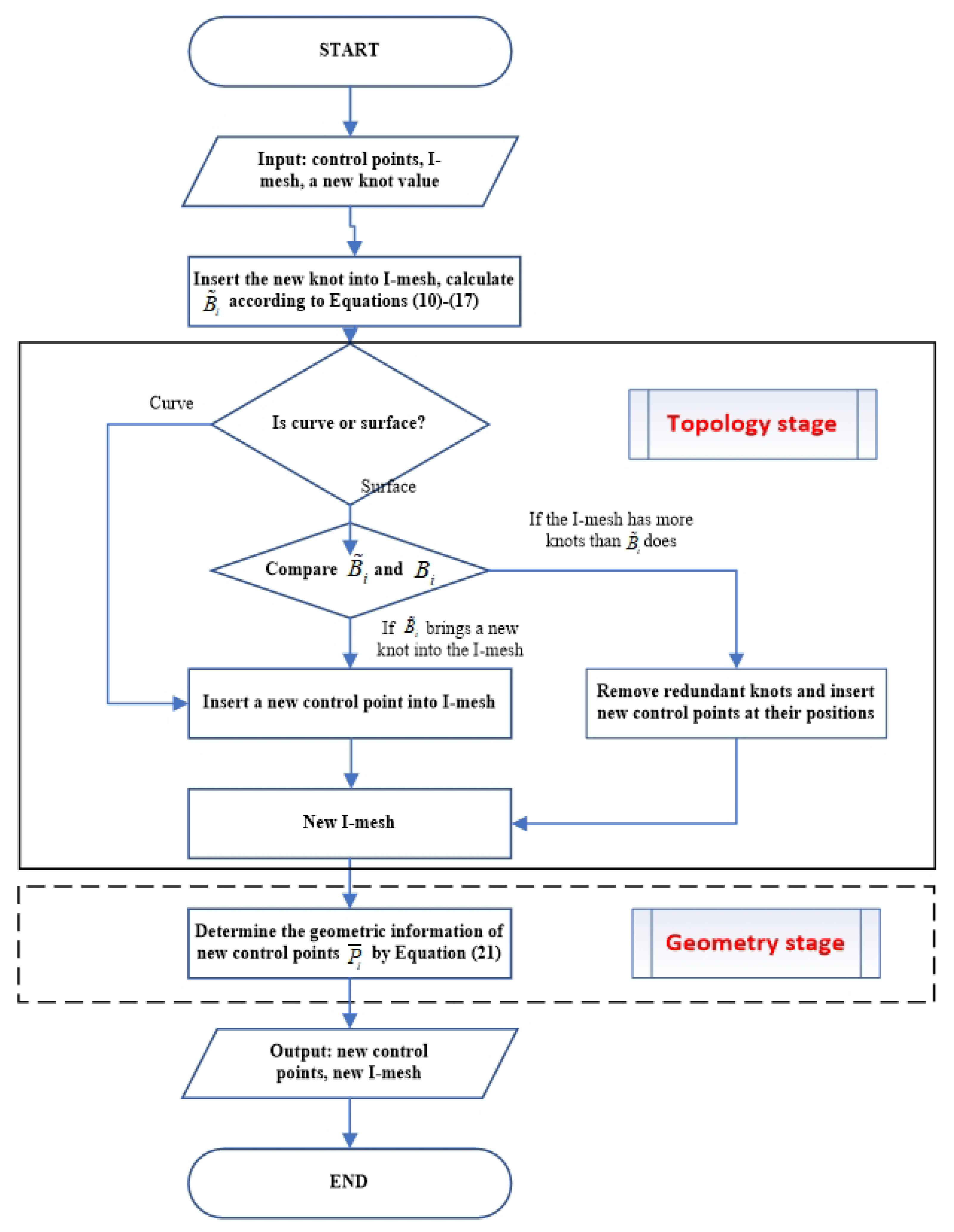
4.2. Local Refinement Algorithm

Similar to the cases of T-splines, the local refinement algorithm of I-splines has two stages, i.e., the topology stage and the geometry one. The main task of the former is to insert control points into an I-mesh without changing the shape of the I-spline, and the latter is to determine the geometry information such as the coordinates of the inserted control points.

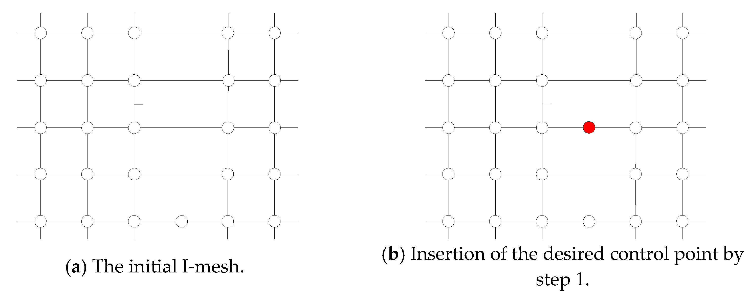
4.2.1. The Topology Stage

There may be two steps to perform the insertion of control points.

Step 1. Insertion of the desired control points into the I-mesh, and determination of ${\tilde{B}}_i$ according to Equations (10)–(17).

For I-spline curves, the desired control points can be inserted directly (see Figure 7). However, in the cases of I-spline surfaces, after step 1, some additional control points may still need to be inserted to satisfy the local refinement condition.

Step 2. Possible insertion of additional control points.

$B_i$ and ${\tilde{B}}_i$ should be compared to judge whether new additional control points should be further inserted or not. Such a judging process may involve two sub-steps: (a) if ${\tilde{B}}_i$ brings a new knot into the I-mesh, a new control point should be inserted on it; (b) in the knot vector of ${\tilde{B}}_i$, if the I-mesh has more knots than ${\tilde{B}}_i$ does, one needs to remove these knots away and then insert new control points at their positions, which will launch a new process of judgment from the case (a) again until no more additional control points are needed.

It deserves noting that the judging process in sub-steps 2(a) and 2(b) will not go into infinite cycling, because the quantity of additional control points is always limited for a specific I-spline.

Two examples are given in Figure 8 and Figure 9 to demonstrate the process of control point insertion in two 2D I-spline topologies, respectively. In the case of Figure 8, only one additional control point is needed to be inserted, and only sub-step 2(a) is employed to perform the additional insertion. However, in the case of Figure 9, two additional control points are required, and both sub-steps 2(a) and 2(b) are involved in the additional insertions.

4.2.2. The Geometry Stage

Let $P^1={\displaystyle \sum _{i=1}^{\overline{n}}{\overline{P}}_i{\overline{B}}_i}$ be the refined version of the original I-spline given in Equation (1). Then, it can be inferred that

$${\displaystyle \sum _{i=1}^n{P}_i{B}_i}={\displaystyle \sum _{i=1}^{\overline{n}}{\overline{P}}_i{\overline{B}}_i}$$

(19)

Substituting Equation (18) into Equation (19), one obtains

$${\displaystyle \sum _{i=1}^n{P}_i}\left({\displaystyle \sum _{k=1}^K{c}_k^{(i)}{\overline{B}}_k}\right)={\displaystyle \sum _{i=1}^{\overline{n}}{\overline{P}}_i {\overline{B}}_i}$$

(20)

Equation (20) can be recast into

$$\left[\begin{array}{cccc}{\overline{B}}_1& {\overline{B}}_2& \cdots & {\overline{B}}_{\overline{n}}\end{array}\right]M\left[\begin{array}{c}{P}_1\\ P_2\\ ⋮\\ P_n\end{array}\right]=\left[\begin{array}{cccc}{\overline{B}}_1& {\overline{B}}_2& \cdots & {\overline{B}}_{\overline{n}}\end{array}\right]\left[\begin{array}{c}{\overline{P}}_1\\ {\overline{P}}_2\\ ⋮\\ {\overline{P}}_{\overline{n}}\end{array}\right]$$

(21)

where $M$ is a coefficient matrix, and $c_k^{(i)}$ ($k=1,2,\cdots ,\overline{n}$; $i=1,2,\cdots ,n$) are its elements.

It follows from Equation (21) that

$${\left[\begin{array}{cccc}{\overline{P}}_1& {\overline{P}}_2& \cdots & {\overline{P}}_{\overline{n}}\end{array}\right]}^T=M{\left[\begin{array}{cccc}{P}_1& P_2& \cdots & P_n\end{array}\right]}^T$$

(22)

The flow chart of the local refinement algorithm is shown in Figure 10.

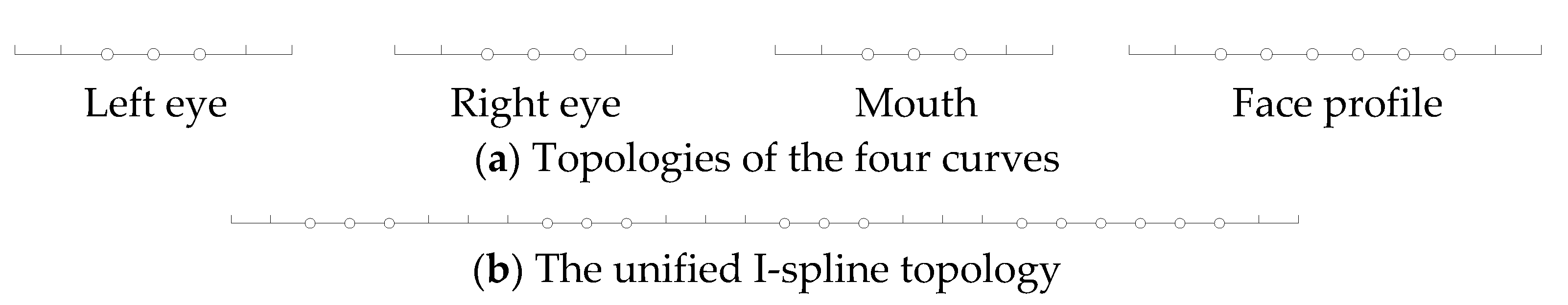
5. Unified Representation of Curves and Surfaces

In geometric modeling, an object may be occasionally represented by separate B-spline curves. For example, the face model in Figure 1 consists of four B-spline curves that are independently defined for the face profile, mouth, and eyes, respectively. Figure 11a illustrates their topologies. The separate representations of these four curves may increase the complexity of animation design. By using I-splines, such complexity can be avoided effectively. As shown in Figure 11b, a unified I-spline topology may be constructed by connecting the four topologies in Figure 11a one by one directly. It is seen that the twelve boundary knots of the separate topologies have been transformed into nine naked knots in the unified topology. The control points and their blending functions of the face profile, mouth, and eyes keep unchanged after the transformation. Therefore, the original face model can be represented by the unified I-spline in Figure 11b.

In conventional geometric modeling, a surface and a curve are generally represented by separate B-splines. Their independent mathematical representations inevitably bring about some troubles to subsequent treatments. By using I-splines, such troubles can be avoided. For example, the surface and the boundary curves of the car model in Figure 2 have their independent topologies as shown in Figure 12a. Here, based on the idea of I-splines, naked knots may be introduced to connect the topology of the surface with those of the two curves to form a unified I-spline topology (see Figure 12b). In this way, the unified I-spline representation is constructed for the surface and the boundary curves of the car model.

Here we demonstrate a specific application of I-spline in CAD (see Figure 13). The original model is the famous Utah Teapot, composed of seven NURBS surfaces (Figure 13a), and their control meshes are shown in Figure 13b. We separate the pot lid from the body to show the convenience of the I-spline in the unified representation of separated surfaces. The topology of NURBS requires seven independent control meshes (Figure 14a), while the I-spline only needs one I-mesh (Figure 14b).

6. Conclusions

The present paper develops a new theoretical tool named I-spline for the unified representation of curves and/or surfaces. The definitions of naked knot and I-mesh are put forward at first, and the concept of I-spline is then set up by inserting naked knots among the control points of B-splines or T-splines. Finally, two examples are presented to demonstrate the effectiveness and versatility of I-splines in uniformly describing curves and surfaces.

I-spline is an extension of NURBS and T-spline, which provides a unified parametric domain for complex models consisting of separate curves and surfaces. This feature can improve the input conditions of CAD downstream applications, optimize the storage space, and simplify the subsequent analysis. Based on the above advantages, I-spline has great potential in the field of geometric modeling and isogeometric analysis. It deserves noting that a lot of investigations such as algorithm improvement and transplantation still need to be conducted to apply the I-spline tool in CAD modeling and even computer animation.

References

1. Cohen, E.; Riesenfeld, R.F.; Elber, G. Geometric Modeling with Splines: An Introduction; AK Peters: Natick, MA, USA, 2001. [Google Scholar]
2. Piegl, L.; Tiller, W. The NURBS Book; Springer: New York, NY, USA, 1997. [Google Scholar]
3. Doo, D.; Sabin, M. Behaviour of recursive division surfaces near extraordinary points. Comput. Aided Des. 1978, 10, 356–360. [Google Scholar] [CrossRef]
4. Sederberg, T.W.; Zheng, J.; Bakenov, A.; Nasri, A. T-slines and T-NURCCs. ACM Trans. Graph. 2003, 22, 477–484. [Google Scholar] [CrossRef]
5. Sederberg, T.W.; Cardon, D.L.; Finnigan, G.T.; North, N.S.; Zheng, J.; Lyche, T. T-spline simplification and local refinement. ACM Trans. Graph. 2004, 23, 276–283. [Google Scholar] [CrossRef] [Green Version]
6. Wang, A.; Zhao, G. The Analysis of T-spline Blending Functions Linear Independence. Comput. Aided Des. Appl. 2011, 8, 735–745. [Google Scholar]
7. Li, X.; Zheng, J.; Sederberg, T.W.; Hughes, T.J.R.; Scott, M.A. On linear independence of T-spline blending functions. Comput. Aided Geom. Des. 2012, 29, 63–76. [Google Scholar] [CrossRef]
8. Li, X.; Zhang, J. AS++ T-splines: Linear independence and approximation. Comput. Methods Appl. Mech. Eng. 2018, 333, 462–474. [Google Scholar] [CrossRef]
9. Wang, A.; Zhao, G.; Li, Y. An influence-knot set based new local refinement algorithm for T-spline surfaces. Expert Syst. Appl. 2014, 41, 3915–3921. [Google Scholar] [CrossRef]
10. Scott, M.A.; Li, X.; Sederberg, T.W.; Hughes, T.J. Local refinement of analysis-suitable T-splines. Comput. Methods Appl. Mech. Eng. 2012, 213, 206–222. [Google Scholar] [CrossRef]
11. Zhang, J.; Li, X. Local refinement for analysis-suitable++ T-splines. Comput. Methods Appl. Mech. Eng. 2018, 342, 32–45. [Google Scholar] [CrossRef]
12. Chen, L.; De Borst, R. Adaptive refinement of hierarchical T-splines. Comput. Methods Appl. Mech. Eng. 2018, 337, 220–245. [Google Scholar] [CrossRef] [Green Version]
13. Wang, A.; Zhao, G. An algorithm of determining T-spline classification. Expert Syst. Appl. 2013, 40, 7280–7284. [Google Scholar] [CrossRef]
14. Singh, S.K.; Singh, I.V.; Mishra, B.K.; Bhardwaj, G.; Bui, T.Q. A simple, efficient and accurate Bézier extraction based T-spline XIGA for crack simulations. Theor. Appl. Fract. Mech. 2017, 88, 74–96. [Google Scholar] [CrossRef]
15. Zhu, Y.; Han, X. C2 interpolation T-splines. Comput. Methods Appl. Mech. Eng. 2020, 362, 112835. [Google Scholar] [CrossRef]
16. Hughes, T.J.; Cottrell, J.A.; Bazilevs, Y. Isogeometric analysis: CAD, finite elements, NURBS, exact geometry and mesh refinement. Comput. Methods Appl. Mech. Eng. 2005, 194, 4135–4195. [Google Scholar] [CrossRef] [Green Version]
17. Bazilevs, Y.; Calo, V.M.; Cottrell, J.A.; Evans, J.A.; Hughes, T.J.R.; Lipton, S.; Scott, M.A.; Sederberg, T.W. Isogeometric analysis using T-splines. Comput. Methods Appl. Mech. Eng. 2010, 199, 229–263. [Google Scholar] [CrossRef] [Green Version]
18. Cottrell, J.; Hughes, T.J.R.; Bazilevs, Y. Isogeometric Analysis: Toward Integration of CAD and FEA; John Wiley & Sons, Ltd.: Hoboken, NJ, USA, 2009. [Google Scholar]
19. Casquero, H.; Liu, L.; Zhang, Y.; Reali, A.; Kiendl, J.; Gomez, H. Arbitrary-degree T-splines for isogeometric analysis of fully nonlinear Kirchhoff–Love shells. Comput. Aided Des. 2017, 82, 140–153. [Google Scholar] [CrossRef]
20. Liu, Z.; Cheng, J.; Yang, M.; Yuan, P.; Qiu, C.; Gao, W.; Tan, J. Isogeometric analysis of large thin shell structures based on weak coupling of substructures with unstructured T-splines patches. Adv. Eng. Softw. 2019, 135, 102692. [Google Scholar] [CrossRef]
21. Chouliaras, S.P.; Kaklis, P.D.; Kostas, K.V.; Ginnis, A.I.; Politis, C.G. An Isogeometric Boundary Element Method for 3D lifting flows using T-splines. Comput. Methods Appl. Mech. Eng. 2021, 373, 113556. [Google Scholar] [CrossRef]
Figure 1. A face model.
Mathematics 09 01019 g001
Figure 2. Part of a car model.
Mathematics 09 01019 g002
Figure 3. A cubic B-spline curve and its topology.
Mathematics 09 01019 g003
Figure 4. I-spline topologies.
Mathematics 09 01019 g004
Figure 5. Control points in I-meshes.
Mathematics 09 01019 g005
Figure 6. The knot vector for a control point of cubic I-splines.
Mathematics 09 01019 g006
Figure 7. Control point insertion in the topology of an I-spline curve.
Mathematics 09 01019 g007
Figure 8. Control point insertion in a 2D I-spline topology.
Mathematics 09 01019 g008
Figure 9. Control point insertion in another 2D I-spline topology.
Mathematics 09 01019 g009aMathematics 09 01019 g009b
Figure 10. Local refinement of I-splines
Mathematics 09 01019 g010
Figure 11. Unified representation of the B-spline curves of the face model.
Mathematics 09 01019 g011
Figure 12. Unified representation of the B-spline surface and curves of the car model.
Mathematics 09 01019 g012
Figure 13. Utah Teapot, the symbol of computer graphics.
Mathematics 09 01019 g013
Figure 14. Unified representation of seven separate NURBS models.
Mathematics 09 01019 g014aMathematics 09 01019 g014b
Publisher’s Note: MDPI stays neutral with regard to jurisdictional claims in published maps and institutional affiliations.