Advanced Metaheuristic Method for Decision-Making in a Dynamic Job Shop Scheduling Environment

Abstract

As a well-known NP-hard problem, the dynamic job shop scheduling problem has significant practical value, so this paper proposes an Improved Heuristic Kalman Algorithm to solve this problem. In Improved Heuristic Kalman Algorithm, the cellular neighbor network is introduced, together with the boundary handling function, and the best position of each individual is recorded for constructing the cellular neighbor network. The encoding method is introduced based on the relative position index so that the Improved Heuristic Kalman Algorithm can be applied to solve the dynamic job shop scheduling problem. Solving the benchmark example of dynamic job shop scheduling problem and comparing it with the original Heuristic Kalman Algorithm and Genetic Algorithm-Mixed, the results show that Improved Heuristic Kalman Algorithm is effective for solving the dynamic job shop scheduling problem. The convergence rate of the Improved Heuristic Kalman Algorithm is reduced significantly, which is beneficial to avoid the algorithm from falling into the local optimum. For all 15 benchmark instances, Improved Heuristic Kalman Algorithm and Heuristic Kalman Algorithm have obtained the best solution obtained by Genetic Algorithm-Mixed. Moreover, for 9 out of 15 benchmark instances, they achieved significantly better solutions than Genetic Algorithm-Mixed. They have better robustness and reasonable running time (less than 30 s even for large size problems), which means that they are very suitable for solving the dynamic job shop scheduling problem. According to the dynamic job shop scheduling problem applicability, the integration-communication protocol was presented, which enables the transfer and use of the Improved Heuristic Kalman Algorithm optimization results in the conventional Simio simulation environment. The results of the integration-communication protocol proved the numerical and graphical matching of the optimization results and, thus, the correctness of the data transfer, ensuring high-level usability of the decision-making method in a real-world environment.

1. Introduction

The use of evolutionary computational methods has been used in decision-making processes in production systems for many years. Heuristic and metaheuristic methods enable obtaining satisfactorily good optimization results for a wide variety of NP-hard decision problems, where a decision problem H is NP-hard when for every problem L in NP, there is a polynomial-time many-one reduction from L to H. The globalized market and digitally supported industry, regardless of the type of production, from the most basic job shop to mass-personalized production, aim to optimize production systems. The paper presents a new metaheuristic method based on the Heuristic Kalman Algorithm [1] which enables optimal scheduling of Dynamic Job Shop Scheduling Problem (DJSSP), and the exchange and use of optimization results in a conventional simulation environment. Within the DJSSP optimization problem, thoroughly describes a real dynamic production system in which three dynamic events occur: The arrival of new orders, machine breakdowns and changes in operations’ process times. Unlike the job shop optimization problem, where orders are static and known in advance, it is necessary to change the scheduling of orders due to dynamic events in the DJSSP optimization problem dynamically and thus ensure optimal operation of the production system.

In the past, DJSSP researchers most often solved the optimization problem with dispatching rules [2], focusing on individual dynamic events [3] (the effects of only one dynamic event are evaluated). Such approaches solved datasets of smaller dimensions satisfactorily but had larger deviations to optimal solutions for more complex optimization problems. The scheduling of job orders from the basic optimization parameter, achieving the minimum flow times of orders, was upgraded by assigning the due date parameter of orders and, consequently, the parameter of job tardiness [4]. At the same time, the dispatching rules became less and less successful, as they only solved the optimization problem well theoretically, especially with a loose due date allowance factor [5]. The trend indicated the need to introduce evolutionary computation methods, which started initially with basic genetic algorithm decision logic [6]. Basic approaches of evolutionary computation methods proved to be useful tools in complex optimization problems in single-criteria optimization [7] in connection with discrete simulation methods [8]. Different researchers, either present the development of new optimization approaches or discrete simulation models that allow the evaluation of dynamic events within conventional simulation tools. The connectivity between self-developed decision-making methods and a discrete simulation model which represents a real-world production system is not found in the literature when evaluating DJSSP.

The development of decision-making methods for solving the DJSSP optimization problem has been extended from single-objective to multi-objective decision-making, where the basic optimization problem is extended to the dynamic flexible job shop scheduling problem (DFJSSP) [9]. The dynamic events represented by machine breakdowns (MB), new jobs arrivals (NJA) and changes in operations process times (PTC) affect different production parameters, and, in DFJSSP in particular, the choice of machine suitable for performing an individual operation must be made [10]. The complexity of choosing the most suitable machine when a dynamic event occurs, in addition to its complexity, further increases the level of need to use evolutionary computation methods [11]. The lack of appropriate mathematical modeling, from the point of view of the correct optimization problem mathematical structure, can represent an irregularity in the operation of evolutionary methods, which intensifies with increasing complexity [12]. Only an appropriate definition of the research problem enables satisfactory good optimization results, capable of compensating for various optimization parameters [13]. Consideration of dynamic events is important if we want to achieve optimally planned and scheduled DJSSP [14]. Dynamic events specific to the real-world production environment must be transferred to simulation models via decision methods [15]. So far this is a well-researched problem in the basic Job Shop Scheduling Problem (JSSP) [16], where the optimization results are satisfactory [17]. Unlike JSSP, the DJSSP literature still does not provide a solution for a data transfer protocol between the optimization algorithm and the conventional simulation environment.

The research work presents a new metaheuristic method for scheduling DJSSP; the method is based on IHKA [18] with a new cellular neighbor network structure, which enables solving DJSSP satisfactorily. A holistic treatment of all three key dynamic events (MB, NJA and PTC), and the evaluation of differently complex datasets (datasets classified into small, medium and large datasets) allows the efficiency and robustness evaluation of the new decision method. Given that the DJSSP represents the characteristics of a real-world production system, the research work represents the integration-communication protocol of optimization results’ integration into the conventional Simio simulation environment, as presented in Figure 1. With the data transfer between the decisive IHKA algorithm and the simulation model in Simio, it is possible to evaluate the DJSSP optimization problem comprehensively from the various production parameters. The research work shows the evaluation of parameters: Machine utilization, machine process time and orders’ flow time. Validation of optimization and simulation results, however, can confirm or refute the importance of proper DJSSP planning and scheduling.

This research paper is organized as follows: in the second section, a problem description of DJSSP with corresponding mathematical model representation is given. This section is followed by the third section, where a newly proposed metaheuristic algorithm IHKA is presented. Next, the experimental design section including the application of IHKA to DJSSP in terms of the evaluation process and simulation model structure proposal is presented. In section five detailed numerical and graphical results of algorithm comparisons are made, followed by the evaluation of the simulation model approach in terms of transformation of optimization results from IHKA to conventional simulation modeling environment. Finally, discussion and conclusions are presented, evaluating results, suggestions, and opportunities for future work.

2. Dynamic Job Shop Scheduling Problem

A Dynamic Job Shop Scheduling Problem (DJSSP) is a combinatorial optimization problem in which we have $n$ job orders given in the introduction and $n^{\prime }$ job orders that arrive after the start of scheduling the $n$ number of job orders. All job orders ($n$ and $n^{\prime }$) must be executed on $m$ available machines, considering the limitations of the DJSSP optimization problem [19]:

• All machines from a set of $m$ are available at time 0;
• An individual operation can only be performed on one machine at a time;
• A single machine $i$ can only perform one operation at a time;
• The operation performed on machine $i$ can only be interrupted when there is a dynamic event of machine breakdown appearing;
• The next operation can be performed only when the previous one is completed;
• The process times of the operation and the assigned machine $i$ are known in advance. During individual operation, the processing time may change due to a dynamic event of changing the original operation processing time;
• The original operation processing time;
• Setup times do not depend on the operation execution sequence and the machine on which the operation will be performed, but are included in the processing time of the operation;
• Transport time between machines is 0.

Problem formulation was made using the following notations for decision variables, datasets and parameters:

$j$	initial jobs $\left(j=1, \dots , n\right)$
$j^{\prime }$	new jobs $\left(j^{\prime }=1, \dots , n^{\prime }\right)$
$i$	machines $\left(i=1, \dots , m\right)$
$A$	set of routing constraints $\left(i,j\right)\to \left(h,j\right)$
$A^{\prime }$	set of new jobs’ routing constraints $\left(i,j^{\prime }\right)\to \left(h,j^{\prime }\right)$
$p_{ij}$	process time of operation $\left(i, j\right)$
${p^{\prime }}_{i{j}^{\prime }}$	process time of new job operation $\left(i, j^{\prime }\right)$
$c_{ij}$	competition time of job j on machine $i$
${c^{\prime }}_{i{j}^{\prime }}$	competition time of new job j’ on machine $i$
$y_{ij}$	starting time of operation $\left(i, j\right)$
${y^{\prime }}_{i{j}^{\prime }}$	starting time of new operation $\left(i, j^{\prime }\right)$
$rp$	the start time of the rescheduled job order
$t{m}_i$	the start that the machine $i$ will be idled at the start of rescheduling job order

In the mathematical description of the single-objective optimization problem, the DJSSP focuses on the minimizing job’s makespan (completion time of all jobs) $C_{max}$, where $c_{ij}$ is the completion time of job $j$ on one machine $i$, described by Equation (1).

$$C_{max}=\left(c_{ij}, i=1, \dots , n\right)$$

(1)

Two constraints (Equations (2) and (3)) ensure that $C_{max}$ is greater than or equal to the completion time of job $j$ and new job $j^{\prime }$ on machine $i$.$i$.

$$C_{max}\ge c_{ij},\mathrm{where} i=1, \dots , m \mathrm{and} j=1, \dots , n$$

(2)

$$C_{max}\ge {c^{\prime }}_{i{j}^{\prime }},\mathrm{where} i=1, \dots , m \mathrm{and} j^{\prime }=1, \dots , n^{\prime }$$

(3)

The makespan of individual operation of orders $n$ and new orders $n^{\prime }$ is determined by Equations (4) and (5).

$$c_{ij}=y_{ij}+p_{ij} \mathrm{where} i=1, \dots , m \mathrm{and} j=1, \dots , n$$

(4)

$${c^{\prime }}_{i{j}^{\prime }}={y^{\prime }}_{i{j}^{\prime }}+{p^{\prime }}_{i{j}^{\prime }}, \mathrm{where} i=1, \dots , m \mathrm{and} j^{\prime }=1, \dots , n^{\prime }$$

(5)

Equations (6) and (7) define the optimization problem constraint condition that the next operation can be performed only when the previous one is completed.

$$y_{hj}-y_{ij}\ge p_{ij} \mathrm{for} \mathrm{all} \left(i,j\right)\to \left(h,j\right)\in A$$

(6)

$${y^{\prime }}_{h{j}^{\prime }}-{y^{\prime }}_{i{j}^{\prime }}\ge {p^{\prime }}_{i{j}^{\prime }} \mathrm{for} \mathrm{all} \left(i,j^{\prime }\right)\to \left(h,j^{\prime }\right)\in A^{\prime }$$

(7)

In addition, some constrains, presented by Equations (8)–(11), must be made according to requirement that only one job can be processed on a machine at any time.

$$M{z}_{ijk}+\left(y_{ij}-y_{ik}\right)\ge p_{ik}, \mathrm{where} \left(i=1, \dots , m, 1\le j\le k\le n\right)$$

(8)

$$M{z}_{i{j}^{\prime }k}+\left({y^{\prime }}_{i{j}^{\prime }}-{y^{\prime }}_{ik}\right)\ge {p^{\prime }}_{ik}, \mathrm{where} \left(i=1, \dots , m, 1\le j^{\prime }\le k\le n\right)$$

(9)

$$M\left(1-z_{ijk}\right)+\left(y_{ik}-y_{ij}\right)\ge p_{ij}, \mathrm{where} \left(i=1, \dots , m, 1\le j\le k\le n\right)$$

(10)

$$M\left(1-z_{i{j}^{\prime }k}\right)+\left({y^{\prime }}_{ik}-{y^{\prime }}_{ij}\right)\ge {p^{\prime }}_{i{j}^{\prime }}, \mathrm{where} \left(i=1, \dots , m, 1\le j^{\prime }\le k\le n\right)$$

(11)

where conditions: $z_{ijk}=1$, if $J_j$ precedes $J_k$ on machine $M_i$ ($z_{ijk}=0$, otherwise), $z_{i{j}^{\prime }k}=1$, if ${J^{\prime }}_{j^{\prime }}$ precedes ${J^{\prime }}_k$ on machine $M_i$ ($z_{i{j}^{\prime }k}=0$, otherwise), $t_{ij}=1$, if $J_j$ will be processed on machine $M_i$ after rescheduling ($t_{ij}=0$, otherwise) and $t_{i{j}^{\prime }}=1$, if ${J^{\prime }}_{j^{\prime }}$ will be processed in machine $M_i$ after rescheduling ($t_{i{j}^{\prime }}=0$, otherwise).

The start time of the rescheduled job orders and the start time of the machine $i$ at the start of the rescheduled job orders is defined by Equations (12) and (13).

$$y_{ij}\ge \left(t{m}_i+rp\right)\ast t_{ij}, \mathrm{where} \left(i=1, \dots , m \mathrm{and} j=1, \dots , n\right)$$

(12)

$${y^{\prime }}_{i{j}^{\prime }}\ge \left(t{m}_i+rp\right)\ast t_{i{j}^{\prime }}, \mathrm{where} \left(i=1, \dots , m \mathrm{and} j^{\prime }=1, \dots , n^{\prime }\right)$$

(13)

As stated in the literature [19] dynamic scheduling can be divided into reactive, predictive-reactive, or pro-active scheduling. This paper uses the predictive-reactive scheduling approach incorporated in the proposed metaheuristic algorithm. For a more real-world usable method, the continuous rescheduling approach was added, where rescheduling is performed each time a dynamic event, new job $n^{\prime }$, arrives. The continuous rescheduling approach gives advantages when the optimization results of DJSSP are transferred into the simulation modeling environment.

3. Metaheuristic Algorithm

A metaheuristic algorithm is introduced in order to solve the DJSSP. Following the introduction of the original metaheuristic algorithm, an improved version is proposed.

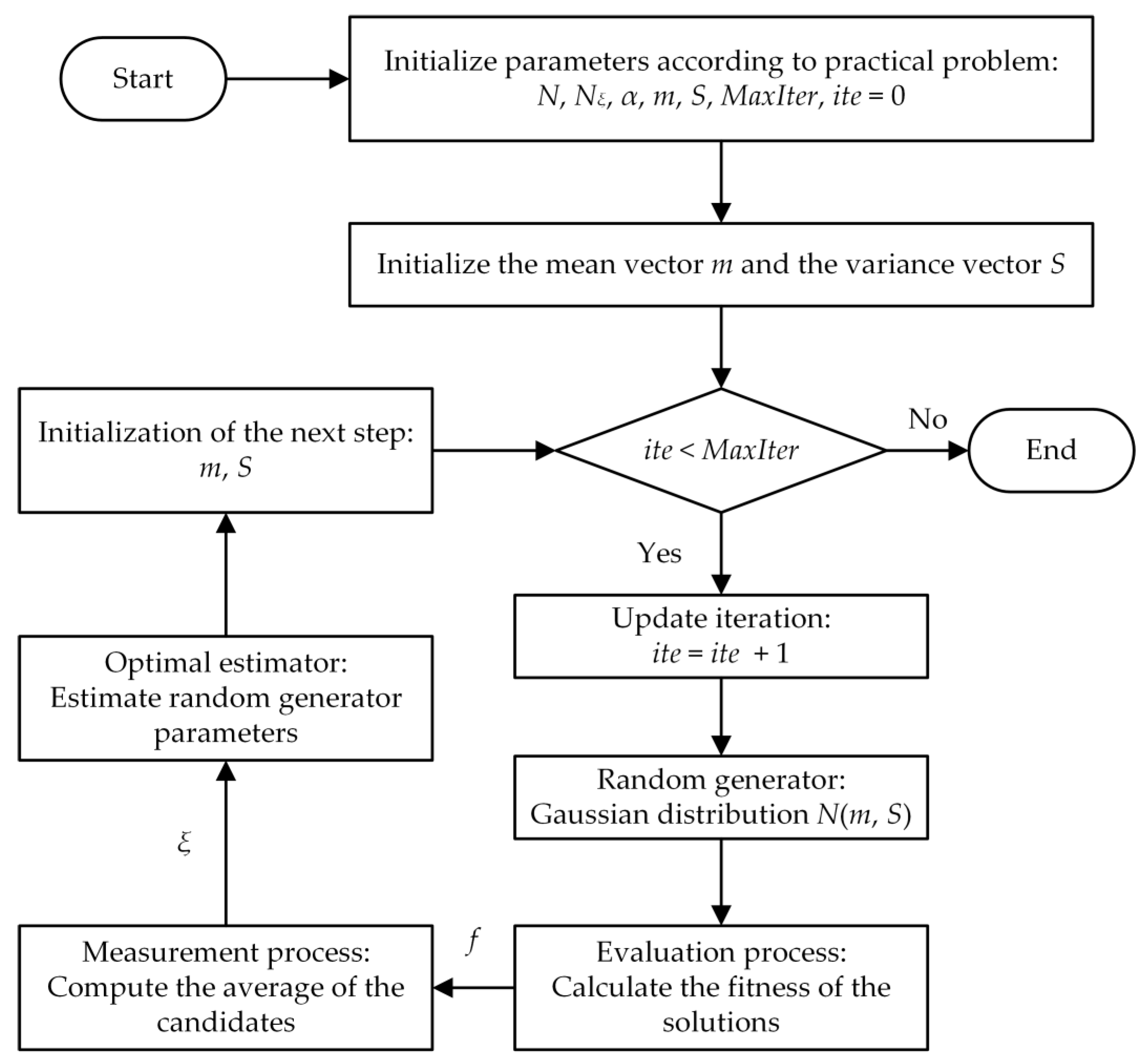
3.1. Heuristic Kalman Algorithm

The Heuristic Kalman Algorithm (HKA) is a Kalman filtering-based heuristic approach, which has been proposed by Toscano and Lyonnet for solving continuous and non-convex optimization problems [1,20]. The HKA is very easy to use, for only a few parameters (only three) need to be set by the user. In the HKA, the search heuristic is entirely different from other population-based stochastic optimization algorithms, which is explicitly considered in the optimization problem as a measurement process designed to give an estimate of the optimum. Through the measurement process, the HKA develops a specific procedure based on the Kalman estimator to improve the quality of the estimate obtained. In the practical implementation, the HKA needs to initialize parameters first, such as the Gaussian distribution, the user-defined parameters and the stopping rule. During the optimization process of the HKA, first, the Gaussian distribution parametrized by a given mean vector with a given variance–covariance matrix generates the solutions, then the evaluation process of the generated solutions, followed by the measurement procedure, and, finally, the optimum estimator of the parameters of the random generator is introduced for the next generation. Figure 2 shows the flowchart of the HKA [1,20].

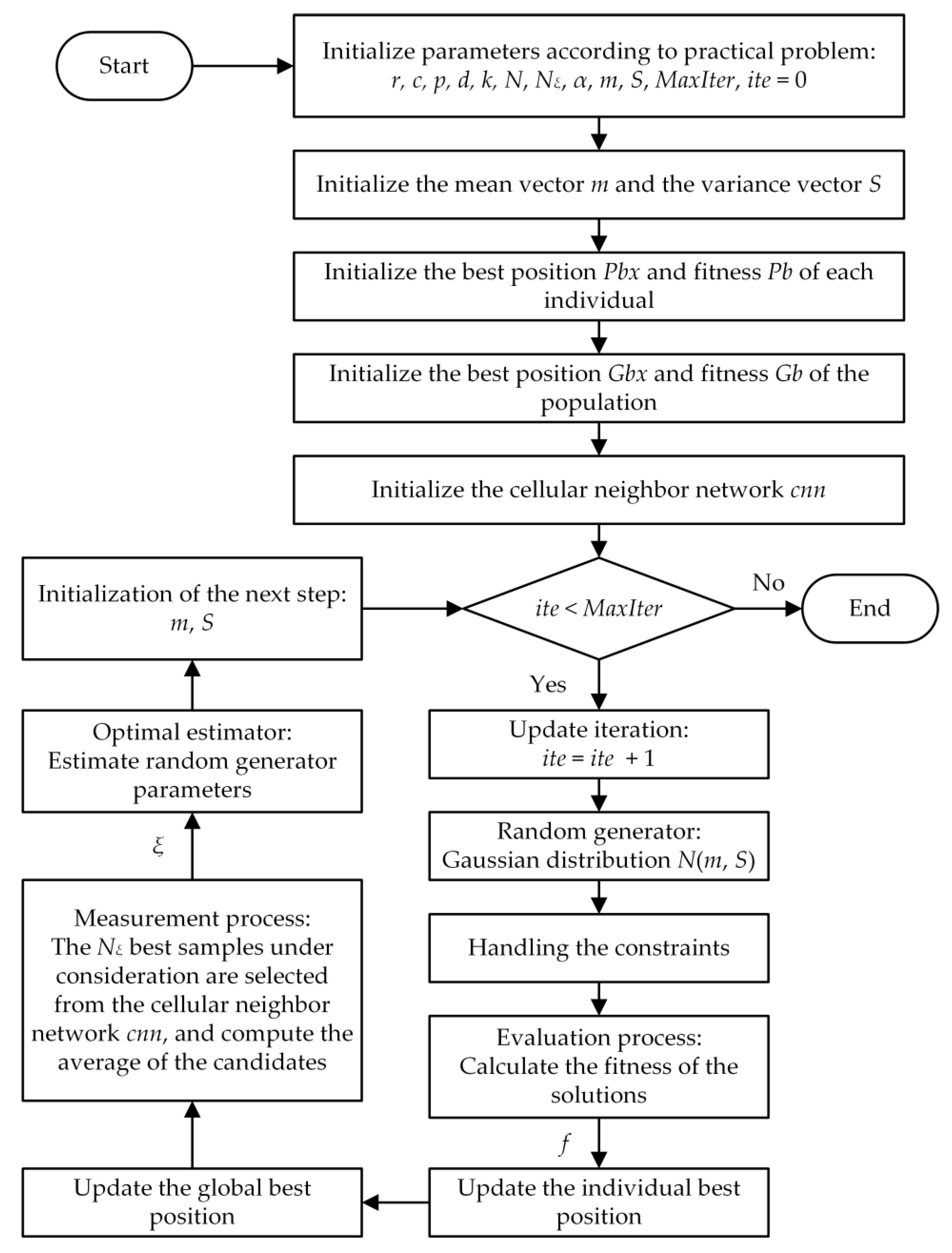
3.2. Improved Heuristic Kalman Algorithm

Due to its very strong convergence, the HKA can easily fall into the local minimum [18,21]. Therefore, the HKA needs to be improved. By introducing the cellular neighbor network, this paper proposes an Improved Heuristic Kalman Algorithm (IHKA). In the IHKA, a function is introduced that handles the boundary constraint after the solutions are generated by the Gaussian distribution, then the best position of each individual is stored and updated after the evaluation process of the generated solutions, and, finally, the cellular neighbor network is introduced during the measurement process to select the best samples under consideration. The general pseudo-code of the IHKA is shown in Algorithm 1 and the flowchart of the IHKA is shows in Figure 3 [21].

Algorithm 1. The general pseudo-code of the IHKA.

Step 0: Initialization. Set the number of rows of the cellular neighbor network $r$, the number of columns of the cellular neighbor network $c$, the neighbor type of the cellular neighbor network $nt$, the rewiring probability of the cellular neighbor network $p$, the minimum maximum depth of the cellular neighbor network $d$, the $k$ nearest neighbors of the cellular neighbor network $k$ (Note that $k$ is set to $N_{\xi }-1$), the size of the population $N=r\ast c$, the number of dimensions of the practical problem $Nd$, the number of best samples under consideration $N_{\xi }$, the slowdown coefficient $\alpha$ and the maximum number of iterations $MaxIter$. Initialize the mean vector $m$ and the variance vector $S$ by Equations (14) and (15), respectively. Initialize the best position $Pbx$ and fitness $Pb$ of each individual by Equations (16) and (17). Initialize the best position $Gbx$ and fitness $Gb$ of the population by Equations (18) and (19). Initialize the cellular neighbor network by Algorithm 2: $cnn=createcnn\left(r, c, nt, p, d, k\right)$ where $createcnn$ is a custom function that generates a cellular neighbor network. Step 1: Iteration. for $ite=1: MaxIter$ Step 1.1: Random generator. Generate a population $x$ with $N$ individuals by a Gaussian distribution parametrized by $m$ and $S$: $x=mvnrnd\left(m, diag\left(S\right), N\right)$ where $mvnrnd(.)$ is a function that generates random vectors from the multivariate normal distribution and $diag(.)$ is a function that generates diagonal matrices or diagonals of a matrix. Step 1.2: Handling the constraints of the problem by Equation (20). Step 1.3: Evaluate fitness. Calculate the individual fitness. Step 1.4: Update the individual best position by Equation (21). Step 1.5: Update the global best position. Step 1.6: Measurement process. The $N_{\xi }$ best samples under consideration are selected from the $k$ nearest neighbors of the global best position in the cellular neighbor network, which is composed of the best positions of individuals: $N_{\xi }=Pbx\left(knni\left(cnn, Gbi\right), :\right)$ where $Gbi$ is the global best position index of the current population and $knni$ is a function to find the $k$ nearest neighbors (containing itself) in the cellular neighbor network. Note that neighbors of each individual can be obtained in advance to reduce the running time. Compute the measurement $\xi$ and the variance vector $V$ by Equations (22) and (23). Step 1.7: Optimal estimation. Compute the posterior estimation: the mean vector $m\_pe$ and the variance vector $S\_pe$ by Equations (24)–(29). Step 1.8: Initialize the next step: $m=m\_pe$,$S=S\_pe$ end

3.2.1. Initializing the Variables

In the IHKA, the initialization parameter is followed by the initialization variable. In the process of initializing variables, the mean vector, the variance vector, the best position of each individual and the best position of the population are initialized.

The mean vector and the variance vector are the parameters of the Gaussian distribution generator. To cover the entire search space, they, denoted $m$ and $S$, are initialized as follows [1]:

$$m={\left[\frac{lu\left(1,1\right)+lu\left(2,1\right)}{2},\cdots ,\frac{lu\left(1,j\right)+lu\left(2,j\right)}{2},\cdots ,\frac{lu\left(1,Nd\right)+lu\left(2,Nd\right)}{2}\right]}^T$$

(14)

$$S={\left[{\left(\frac{lu\left(2,1\right)-lu\left(1,1\right)}{6}\right)}^2,\cdots ,{\left(\frac{lu\left(2,j\right)-lu\left(1,j\right)}{6}\right)}^2,\cdots ,{\left(\frac{lu\left(2,Nd\right)-lu\left(1,Nd\right)}{6}\right)}^2\right]}^T$$

(15)

where $lu\left(1, j\right)$ (respectively, $lu\left(2, j\right)$) is the lower (respectively, upper) boundary of the $j$-th dimension of the problem.

The best position of each individual is stored to construct the cellular neighbor network. In the initialization process, the best position and fitness of each individual are initialized. The best position of the individual is initialized as a zero vector. Its fitness is initialized to infinity (respectively, negative infinity) for the minimization (respectively, maximization) problem. For minimization problem, they, denoted $Pbx$ and $Pb$, are initialized as follows:

$$Pbx=zeros\left(N, Nd\right)$$

(16)

$$Pb=inf\left(N, 1\right)$$

(17)

where $zeros$ (respectively, $inf$) is a function that produces a matrix of all zeros (respectively, infinity).

The best position of the population is used to handling the constraints. When a certain dimension of an individual violates the constraints, it may be replaced by the corresponding dimension of the best position of the population. It needs to be used during the first processing of handling the constraints, so it is randomly initialized in the search space. They, denoted $Gbx$ and $Gb$, are initialized as follows:

$$Gbx=lu\left(1,:\right)+\left(lu\left(2,:\right)-lu\left(1,:\right)\right).\ast rand\left(1, Nd\right)$$

(18)

$$Gb=f\left(Gbx\right)$$

(19)

where $rand$ is a function to generate random numbers in the interval (0, 1) and $f$ is a function to evaluate the fitness of the individual.

3.2.2. Handling the Constraints

To handle the boundary constraints, a handling constraints function is introduced in the IHKA. If a dimension value violates the boundary constraint, it will be replaced. According to a large number of preliminary experiments, it has a 50% probability that it will be replaced by a random number. The probability of being replaced by the corresponding dimension value of the global best position is 25%. Otherwise, it is replaced by a boundary value. If it is greater than the upper boundary value, it will be replaced by the upper boundary value, otherwise, it will be replaced by the lower boundary value. Note that, if the boundary value cannot be taken, it will be replaced with a value that is infinitely close to the boundary value. The rule for handling the constraints is used as follows:

$$x\left(i,j\right)=\{\begin{array}{ll}lu\left(1,j\right)+\left(lu\left(2,j\right)-lu\left(1,j\right)\right)\ast rand,\hfill & \hfill ra<0.5\hfill \\ Gbx\left(1,j\right)\hfill & \hfill 0.5\le ra<0.75\hfill \\ lu\left(1,j\right)\hfill & \hfill ra>0.75 \wedge x\left(i,j\right)<lu\left(1,j\right)\hfill \\ lu\left(2,j\right)\hfill & \hfill ra>0.75 \wedge x\left(i,j\right)>lu\left(2,j\right)\hfill \end{array}$$

(20)

where $x\left(i, j\right)$ represents the $j$-th dimension of the $i$-th individual who violated the boundary constraints in the population $x,$ and $ra$ is a random number generated by the random function.

3.2.3. Updating the Individual Best

The best position in the history of each individual is stored in the IHKA. They are used to construct the cellular neighbor network to ensure the convergence of the IHKA. If its fitness is not worse than the original, the newly generated individual will replace the individual at the corresponding position in the cellular neighbor network. The rule for updating the individual best is used as follows:

$$Pb\left(i\right)=\{\begin{array}{ll}f\left(i\right),\hfill & f\left(i\right)\le Pb\left(i\right)\hfill \\ Pb\left(i\right)\hfill & f\left(i\right)>Pb\left(i\right)\hfill \end{array}$$

(21)

where $f\left(i\right)$ represents the fitness of the newly generated individual $i$.

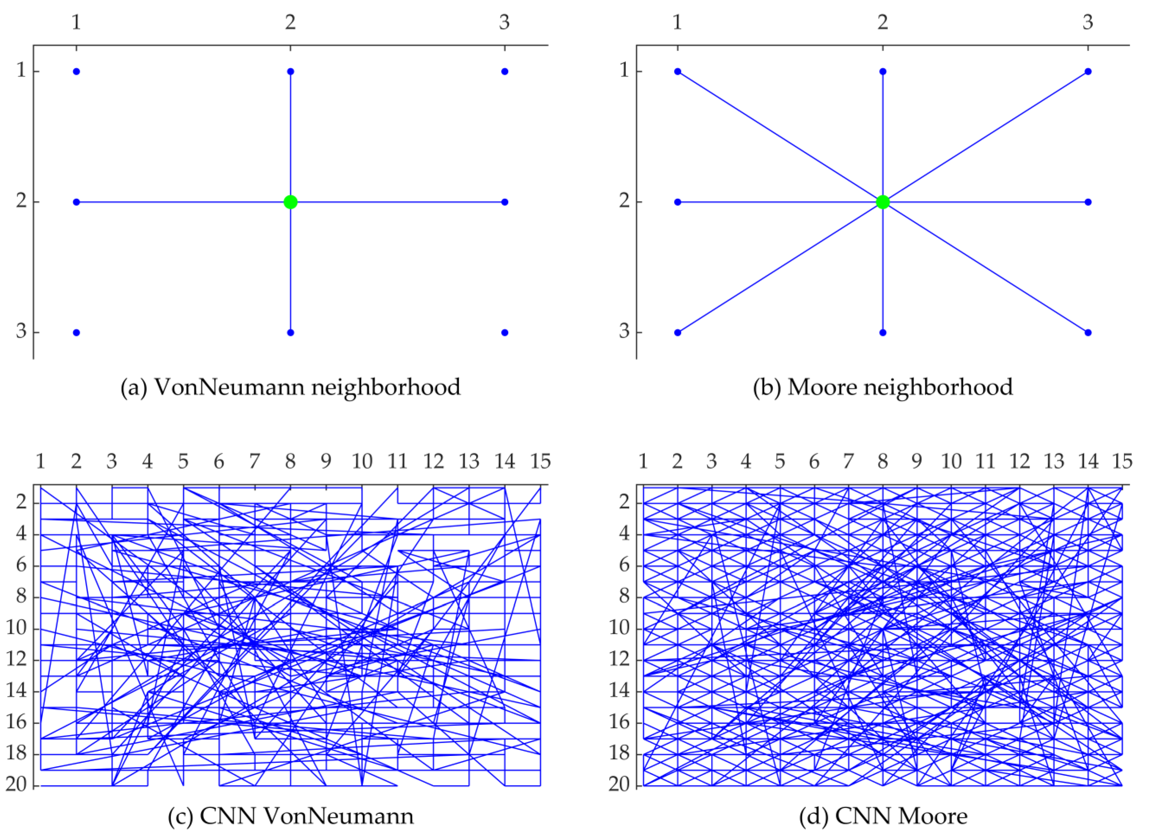
3.2.4. Introducing the Cellular Neighbor Network

During the measurement process, the cellular neighbor network is introduced to select the best samples under consideration in the IHKA. The cellular neighbor network was proposed by Li et al. for a cellular neighbors-based structure can achieve good performance in human society or a network [22]. In the cellular neighbor network, each individual is composed of individuals at corresponding positions in the population. Each individual in the cellular neighbor network uses the best position explored by the corresponding position individual in the population during the optimization process. In a two-dimensional space, there are two well-known structures in the neighborhood of a cell, which are the Von Neumann neighborhood [23] and the Moore neighborhood [24]. Their neighborhood structure is shown in Figure 4a and Figure 4b, respectively. We set the minimum maximum depth of the cellular neighbor network to ensure that each node in the network is connected. The construction of the cellular neighbor network is described in detail in Algorithm 2. The instances of cellular neighbor networks constructed by the proposed algorithm are shown in Figure 4c and Figure 4d, respectively.

Algorithm 2. The general pseudo-code for creating cellular neighbor network.

Input: the number of rows of the cellular neighbor network $r$, the number of columns of the cellular neighbor network $c$, the neighbor type of the cellular neighbor network $nt$, the rewiring probability of the cellular neighbor network $p$, the minimum maximum depth of the cellular neighbor network $d$, the $k$ nearest neighbors of the cellular neighbor network $k$. Output: the cellular neighbor network.Initialize the network. Step 0: Initialize a regular cellular neighbor network based on the type of cellular neighborhood. Step 1: Create the network. Construct a cellular neighbor network based on the rewiring probability of the cellular neighbor network $p$. After cutting, the minimum maximum depths of the two nodes selected for deletion are checked, if the requirements are not met, the disconnection is canceled. Note that this check does not affect the addition of new random connections. Step 2: Obtain $k$ nearest neighbors. Obtain the $k$ nearest neighbors (containing itself) of each node in the network.

3.2.5. Computing the Measurement

In the measurement process, $N_{\xi }$ best samples under consideration are selected, followed by the calculation of the measurement and the variance vector. They, denoted $\xi$ and $V$ are define as follows [1]:

$$\xi =\frac{1}{N_{\xi }}{\sum }_{k=1}^{N_{\xi }}{x}_k$$

(22)

$$V=\frac{1}{N_{\xi }}{\left[{\sum }_{k=1}^{N_{\xi }}{\left(x_{k,1}-{\xi }_1\right)}^2,\cdots ,{\sum }_{k=1}^{N_{\xi }}{\left(x_{k,j}-{\xi }_j\right)}^2,\cdots ,{\sum }_{k=1}^{N_{\xi }}{\left(x_{k,Nd}-{\xi }_{Nd}\right)}^2\right]}^T$$

(23)

3.2.6. Computing the Posterior Estimation

In the optimal estimation process, the mean vector and the variance vector are calculated for the next step. They are the parameters of the Gaussian distribution generator of the next-generation population. They, denoted $m\_pe$ and $S\_pe$, are define as follows [1]:

$$L=S./\left(S+V\right)$$

(24)

$$W={\left(S-L.\ast S\right)}^{0.5}$$

(25)

$$m\_pe=m+L.\ast \left(\xi –m\right)$$

(26)

$$\tau =min\left(1, mean{\left(\sqrt{V}\right)}^2\right)$$

(27)

$$a=\alpha \tau ⁄\left(\tau +max\left(W\right)\right)$$

(28)

$$S\_pe={\left(S^{0.5}+a.\ast \left(W–S^{0.5}\right)\right)}^2$$

(29)

where $L$, $W$ and $\tau$ are unknown vector which have to be determined to ensure optimal estimation, $a$ is the slowdown factor, $mean (.)$ is a function that calculates the mean value and the symbol$./$ (respectively, $.\ast$) stands for a component-wise divide (respectively, product).

4. Experiment Design

In order to verify the performance of the proposed metaheuristic algorithm, this paper designs an experiment. The experiment contains the numerical experiment of the algorithm and the simulation experiment of the optimization results of the algorithm for the benchmark instances of DJSSP.

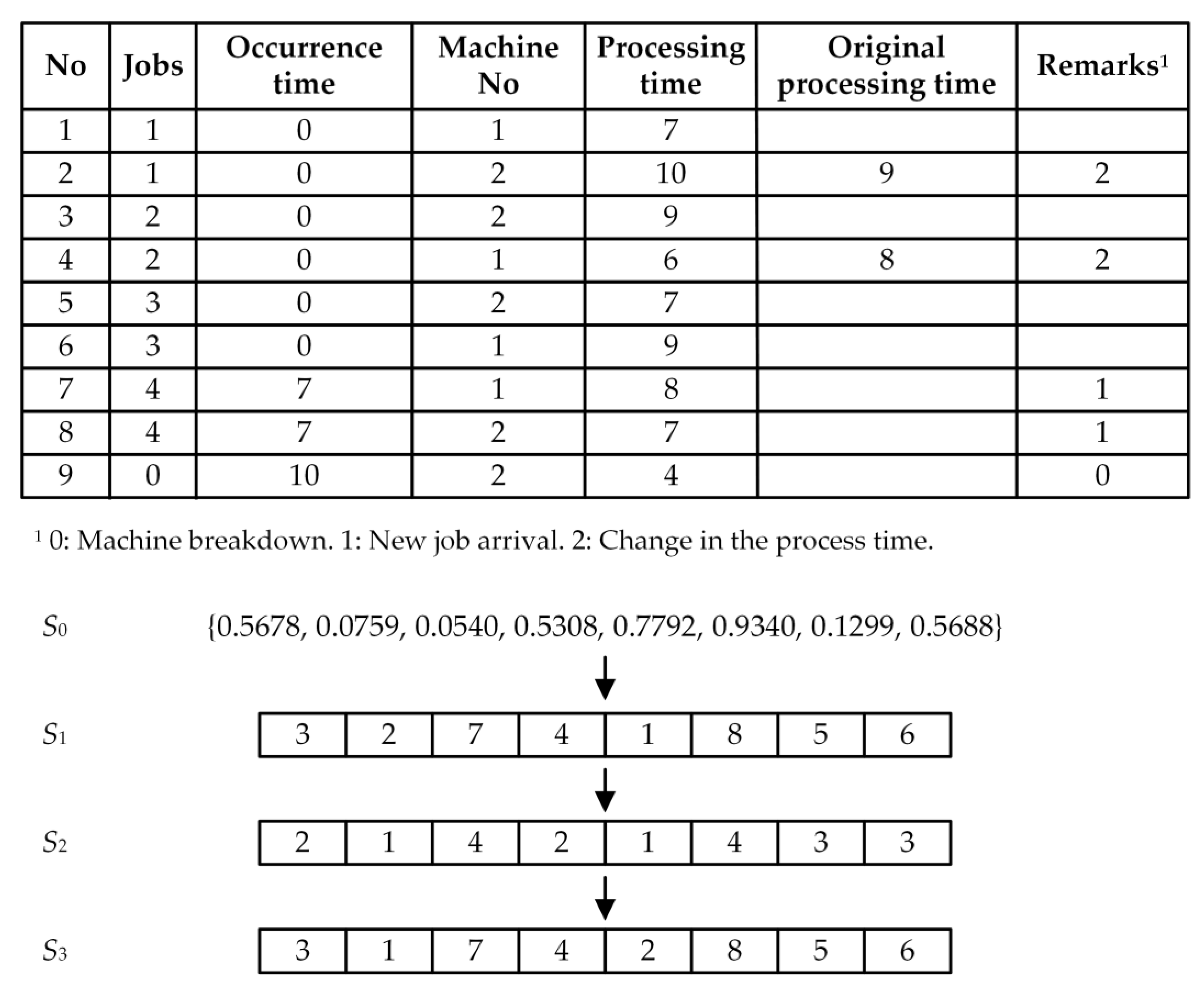
4.1. Applying the Algorithm on DJSSP

The HKA was originally proposed to solve continuous problems, so we introduced the relative position indexing [25] to encode. The instance of the solution encoding is shown in Figure 5. Each dimension of the individual is initialized randomly to an open interval of 0 and 1 (see Figure 5 $S_0$). The position of the individual is transferred into the discrete domain by using the relative position index (see Figure 5 $S_1$). That is, the value of each dimension of the individual represents the priority, the smaller the value, the higher the priority it will be processed with. For instance, in Figure 5 $S_0$, the value of the third (respectively, sixth) position is the smallest (respectively, largest), so its processing priority is the highest (respectively, lowest), that is, it is ranked first (respectively, last) in the processing priority. Then the processing sequence of the jobs can be obtained from the DJSSP Table (see Figure 5 $S_2$). That is, sort the “Jobs” column in the DJSSP Table (not including the rows of the machine breakdowns). In Figure 5 $S_2$, the jobs processing sequence is as follows: (2, 2), (1, 1), (4, 1), (2, 1), (1, 2), (4, 2), (3, 2), (3, 1), where (., .) means job number and machine number. For instance, (2, 2) means job 2 is processed on machine 2. In Figure 5 $S_2$, the $k$-th occurrence of a job number represents the $k$-th operation of the job. Finally, the final solution can be obtained (see Figure 5 $S_3$). In Figure 5 $S_3$, the operations processing sequence is as follows: (3, 2), (1, 1), (7, 1), (4, 1), (2, 2), (8, 2), (5, 2), (6, 1), where (., .) means number (corresponding to the number in the “No” column in the DJSSP Table) and machine number. For instance, (3, 2), means that the third row in the DJSSP Table (job 2) is processed on machine 2.

4.2. Evaluating the Algorithm

In order to evaluate the proposed algorithm, we introduced the benchmark instances of DJSSP and set the parameters of the algorithm.

4.2.1. Selecting the Benchmark Instance

The benchmark instances of DJSSP were selected in order to verify the performance of the proposed algorithm to solve the DJSSP. All selected benchmark instances of DJSSP are from [19], which were generated based on Lawrence static job shop benchmark problem instances. In all the benchmark instances of DJSSP, each instance considers dynamic events such as machine breakdown, new job arrival and change in the processing time. In [19], without considering the arrival of new jobs, 15 benchmark instances of DJSSP are divided into three categories: Small (less than 60), medium (greater than, or equal to 60 and less than 100) and large (greater than, or equal to 100) according to the number of operations. For the benchmark instances of DJSSP see

Table 1. The benchmark instances of DJSSP.

Size Type	No	Size n × m	Number of Operations	Number of Dynamic Operations	Total	Optimal Fitness 1
small	1	5 × 5	25	10	35	51
	2	6 × 5	30	15	45	557
	3	8 × 5	40	5	45	699
	4	10 × 5	50	5	55	624
medium	5	10 × 6	60	6	66	682
	6	15 × 5	75	5	80	1001
	7	10 × 8	80	8	88	1027
	8	10 × 9	90	18	108	1049
large	9	20 × 5	100	5	105	1361
	10	10 × 10	100	10	110	1389
	11	22 × 5	110	15	125	1458
	12	12 × 10	120	10	130	1002
	13	13 × 10	130	10	140	1016
	14	20 × 7	140	14	154	1326
	15	15 × 10	150	20	170	1280

¹ Optimal fitness obtained in [19].

. The detailed data of all the selected benchmark instances of DJSSP can be obtained from [19]. In the benchmark instances of DJSSP, it focuses on the minimizing job’s makespan (completion time) $C_{max}$, described by Equation (1), that is, the optimal fitness.

4.2.2. Defining the Parameters

In this paper, the $MaxIter$ of the IHKA and HKA was set according to a large number of preliminary experiments, and the others were set according to the previous literature. The parameters $r$, $c$, $k$, $N$, $N_{\xi }$ and $\alpha$ were set according to [18,21]. The parameters $p$ and $d$ were set according to [22] and [26], respectively. In the large number of preliminary experiments, the $MaxIter$ was set to a different value, and the algorithm was independently run many times to solve each of the selected 15 benchmark instances, and the convergence process of the algorithm was observed. If it converged after the maximum iteration of each independent run, the $MaxIter$ corresponding to the benchmark instance was determined. According to the large number of preliminary experiments, the $MaxIter$ was set to a different value corresponding to the size type of each benchmark instance. The parameters of the IHKA and HKA are shown in

Table 2. The parameters of the IHKA and HKA.

No	Name	Value	No	Name	Value	No	Name		Value
1	$r$	20	4	$d$	5	7	$N_{\xi }$		10
2	$c$	15	5	$k$	9	8	$\alpha$		0.3
3	$p$	0.5	6	$N$	300	9	$MaxIter$	small	1000
								medium	2000
								large	3000

. The parameters defined in Table 2 will be used in all the experiments.

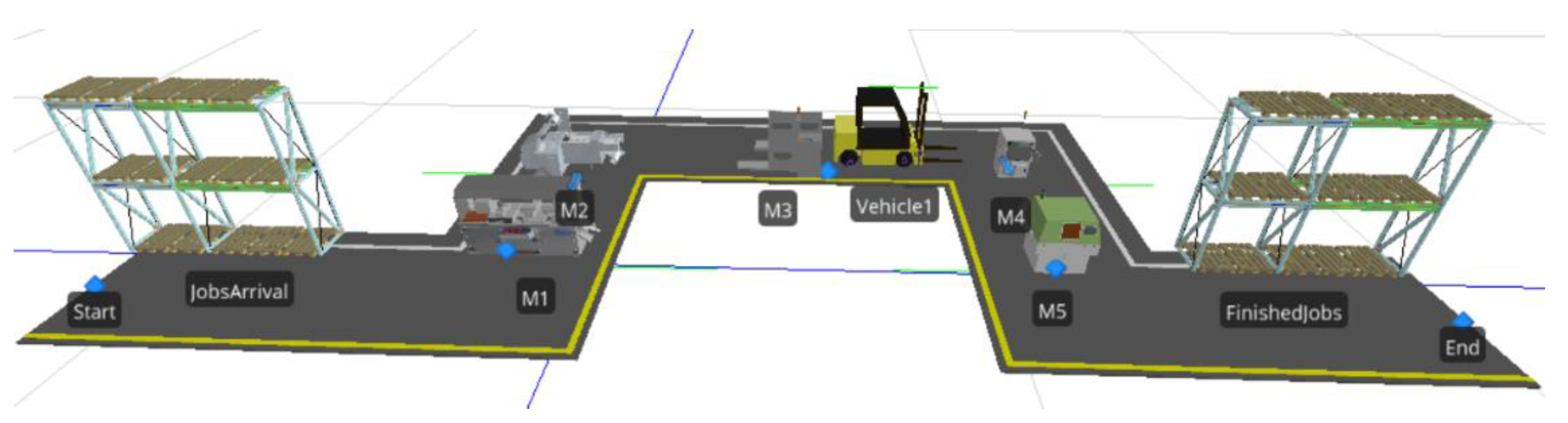
4.3. Transferring Optimization Results to Simulation Evaluation

Given the basic purpose of the DJSSP optimization problem, in which dynamic events such as machine breakdowns (MB), operation process time changes (PTC) and new job arrivals (NJA), occur dynamically, this optimization problem shows the most realistic problem of job shop scheduling using the IHKA, and the high ability to schedule the job and operations of the DJSSP optimization problem has been proven. In the next experimental phase, it is necessary to transfer the optimization results into the real production system environment. To transfer the optimization results of the IHKA to the real-world environment, the simulation modeling method in the commercially available Simio software environment is presented the simulation model of benchmark dataset 6 × 5 is shown in Figure 6. Established communication protocol was introduced when transferring the optimization results of the IHKA to the commercial simulation environment [27].

The simulation model includes five machines (from M₁ to M₅), a warehouse of input material (jobs’ arrival point) and a warehouse of finished products (jobs’ finished point), and the transport of semi-finished orders between stations is provided by a forklift.

Table 3. The scheduling DJSSP results.

Job/Operation	Machine	Start Time (Time Unit)	End Time (Time Unit)	Process Time (Time Unit)	Dynamic Event
J3,1	M4	0	34 + 9 = 43	43	MB
J3,2	M3	69	133	64	/
J3,3	M2	133	156	23	PTC
J3,4	M5	201	293	92	/
J3,5	M1	453	536	83	/
J4,1	M2	21	87 + 5 = 113	92	MB
J4,2	M4	141	210	69	/
J4,3	M3	318	405	87	/
J4,4	M1	405	453	48	PTC
J4,5	M5	484	544	60	/
J7, 1	M4	119	141	22	NJA
J7,2	M2	156	188	32	NJA
J7,3	M1	188	198	10	NJA
J7,4	M3	405	430	25	NJA
J7,5	M5	430	484	54	NJA

shows the optimization results of the IHKA transmitted via the MATLAB-Excel-Simio communication protocol to a data-driven simulation model. The 6 × 5 DJSSP dataset used contains six initial jobs (from J₁ to J₆) and three additional job arrivals (J₇ to J₉). Four jobs are static (J₁, J₂, J₅ and J₆), and in addition five jobs are dynamic (J₃, J₄, J₇, J₈, J₉). In dynamic job J₃, two dynamic events occur: Interruption due to machine breakdown in operation J_3,1, which is 9 min long, and change in process time in operation J_3,3, from the original process time of 19 min to 23 min.

Similar dynamic events occur in job J₄: an interruption is performed due to a machine breakdown in operation J_4,1, with duration of 5 min and a change in process time in operation J_4,4 from the original process time of 93 min to 48 min. The other three dynamic jobs are J₇, J₈ and J₉ represent new job arrivals. In a dynamic machine breakdown event, the simulation model uses a data table with the event time-based interruption function assigned to a specific operation and machine. The time of execution of the breakdown event is defined by the Time to Repair function, in which the repair time value is specified: For J_3,1 the repair time is 9 min, and for J_4,1 the time is 5 min, respectively. This value is added to the initial value of the process time of the operation, and, as a sum, represents the process time of the entire operation. The dynamic event of the change of the operation process time is modeled with a data-driven table of process times, in which the values of the initial and updated process times are given. The simulation model, when new job arrivals appear, obtains data on these via MatLab-Excel-Simio communication, dynamically, according to the performed optimization with the IHKA. The arrival of a new job in the existing order queue is assigned by the new job arrival variable. Despite the fact that the presented simulation model is limited to displaying the 6 × 5 DJSSP dataset, the proposed build-in decision logic is adaptable, and it is possible to change the simulation model continuously according to the characteristics of the devalued production system.

5. Result

The corresponding experimental results were obtained after the experimental design, numerical experiments and simulation experiments were executed in the MATLAB and Simio software.

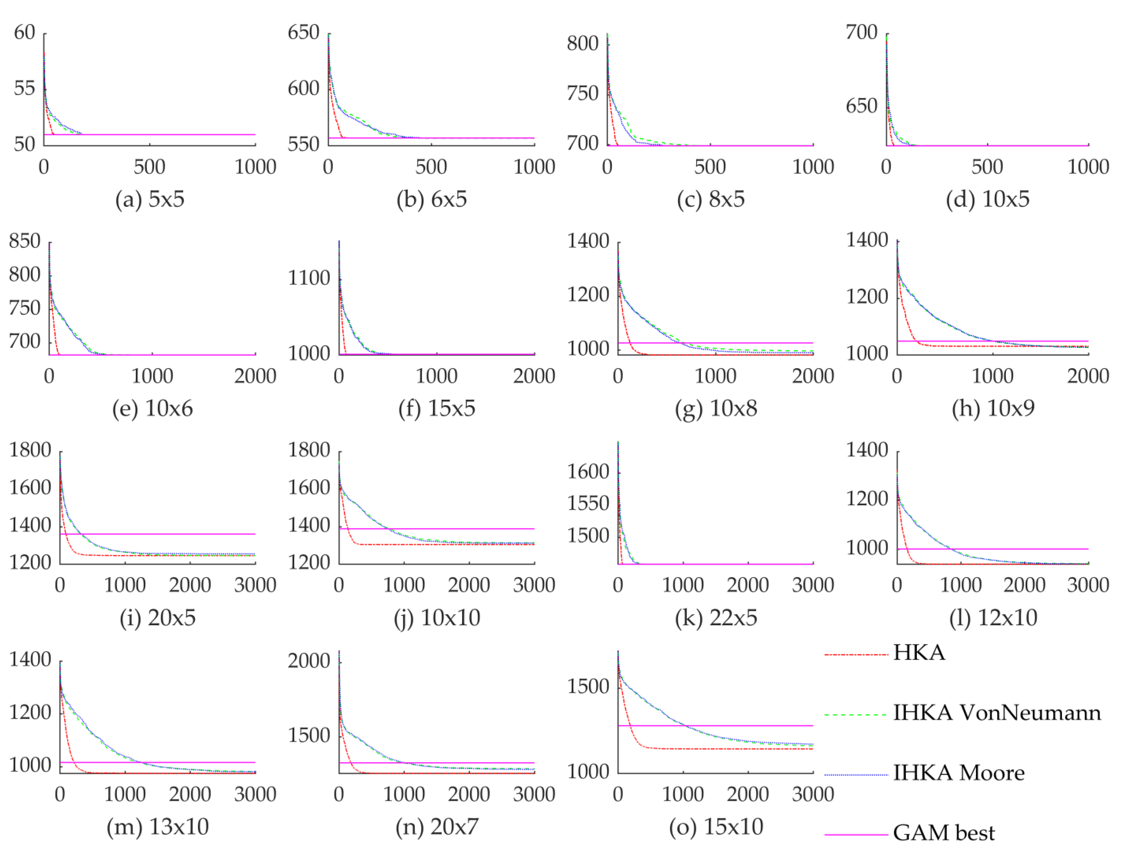
5.1. Results Comparison to Other Algorithms

The original HKA and the Genetic Algorithm-Mixed (GAM) [19] were selected as a comparison to prove the performance of the proposed IHKA to solve the DJSSP. In order to prove the robustness, the IHKA and HKA were run independently, 30 times for each benchmark instance of DJSSP. All the algorithms in this paper are implemented in MATLAB language. All experiments were simulated in version R2020b of MATLAB. The computer used in all experiments was a PC with x64-processor Intel(R) Core(TM) i7-8550U CPU @ 1.80 GHz 1.99 GHz and 16 GB RAM in the environment of the Windows 10 version 20 H2.

Figure 7 shows the IHKA and HKA average convergence of the best solutions for the benchmark instances of DJSSP. The convergence curve in the Figure is the average of 30 independent runs of each algorithm. It can be seen from the Figure that the IHKA reduced the convergence rate significantly, which is beneficial to avoid the algorithm from falling into the local optimum during the optimization process. In the IHKA, the influence of different cellular neighborhood structures on the convergence process is not very obvious. In the IHKA, the average convergence process of 30 independent runs of two cellular neighborhood structures, the Von Neumann neighborhood and the Moore neighborhood, are almost the same. The Figure can also clarify that both HKA and IHKA can converge to the best solution for all benchmark instances of DJSSP. For most of the benchmark instances of DJSSP, such as 10 × 8, 10 × 9, 20 × 5, 10 × 10, 12 × 10, 13 × 10, 20 × 7 and 15 × 10, both IHKA and HKA can converge significantly to the best solution obtained by GAM. Therefore, the convergence performance of IHKA and HKA was clarified to be very good. Moreover, we can also see that, in some instances, such as 10 × 8, 10 × 9, 12 × 10, 13 × 10, 20 × 7 and 15 × 10, the IHKA algorithm still shows a trend of convergence at termination. It means that better solutions may be obtained by increasing the number of iterations of the algorithm for each of these instances.

The computational statistics of the IHKA and HKA on the fitness for the benchmark instances of DJSSP are shown in

Table 4. The computational statistics of the IHKA and HKA on the fitness for the benchmark instances of DJSSP.

Size n × m	GAM Best	HKA					IHKA VonNeumann					IHKA Moore
		Min	Max	Mean	Std.	SR	Min	Max	Mean	Std.	SR	Min	Max	Mean	Std.	SR
5 × 5	51	51	51	51	0	100	51	51	51	0	100	51	51	51	0	100
6 × 5	557	557	557	557	0	100	552	557	556.83	0.91	100	557	557	557	0	100
8 × 5	699	699	699	699	0	100	699	699	699	0	100	699	699	699	0	100
10 × 5	624	624	624	624	0	100	624	624	624	0	100	624	624	624	0	100
10 × 6	682	682	682	682	0	100	682	682	682	0	100	682	682	682	0	100
15 × 5	1001	1001	1001	1001	0	100	1001	1001	1001	0	100	1001	1001	1001	0	100
10 × 8	1027	947	1009	982.17	15.11	100	953	1022	997.47	16.55	100	944	1019	990.77	19.88	100
10 × 9	1049	1005	1059	1030.73	14.17	86.7	1005	1043	1026.73	11.97	100	1005	1052	1027.30	13.28	96.7
20 × 5	1361	1202	1277	1245.90	17.49	100	1217	1282	1246.10	18.32	100	1218	1307	1255.20	18.97	100
10 × 10	1389	1292	1337	1304.90	10.84	100	1287	1360	1313.80	16.62	100	1289	1359	1312.60	18	100
22 × 5	1458	1458	1458	1458	0	100	1458	1458	1458	0	100	1458	1458	1458	0	100
12 × 10	1002	912	981	939.63	17.18	100	914	989	941.33	17.81	100	918	979	940.90	13.60	100
13 × 10	1016	949	1011	974.80	15.95	100	947	1016	981.70	17.95	100	952	1008	980.90	13.60	100
20 × 7	1326	1246	1286	1255.30	11.66	100	1260	1315	1286.40	15.51	100	1246	1324	1281.47	19.42	100
15 × 10	1280	1112	1164	1143.87	14.77	100	1130	1203	1161.77	20.21	100	1122	1246	1171.50	27.12	100

. In Table 4, for each benchmark instance, if the algorithm has the best statistical performance, then the row is bolded, otherwise the minimum value is bolded. It can be clarified from the Table 4 that both the IHKA and HKA performed very well. For most of the benchmark instances of DJSSP, such as 6 × 8, 10 × 8, 10 × 9, 20 × 5, 10 × 10, 12 × 10, 13 × 10, 20 × 7 and 15 × 10, the best solutions obtained by IHKA and HKA were better than those obtained by GAM. As an example, the best solution and the Gantt chart of the 6 × 5 DJSSP with IHKA VonNeumann are given in

Table 5. The best solution of the 6 × 5 DJSSP with IHKA VonNeumann.

Machine 1	Job’s sequence	1	7	5	6	9	2	4	3	8
	Start time	69	188	231	275	370	393	405	453	536
	Finish time	122	198	275	370	393	405	453	536	545
Machine 2	Job’s sequence	1	4	3	7	5	9	6	2	8
	Start time	0	21	133	156	275	324	370	405	447
	Finish time	21	113	156	188	324	334	377	447	496
Machine 3	Job’s sequence	6	1	3	5	8	2	4	7	9
	Start time	0	35	69	133	231	287	318	405	430
	Finish time	35	69	133	231	287	318	405	430	477
Machine 4	Job’s sequence	3	6	7	4	1	8	5	2	9
	Start time	0	43	119	141	210	320	420	447	486
	Finish time	43	119	141	210	265	352	437	486	513
Machine 5	Job’s sequence	2	6	1	3	8	5	7	4	9
	Start time	0	119	180	201	293	324	430	484	544
	Finish time	55	180	201	293	320	420	484	544	552

and Figure 8, respectively. In Figure 8, the yellow is used to represent the period of machine breakdown. For 30 independent runs of all the benchmark instances of DJSSP, the IHKA VonNeumann had a 100% success rate (SR) for obtaining the best solution at least better than that obtained by GAM. Except for the 10 × 9 DJSSP, the success rate of IHKA Moore and HKA was also 100%. In 30 independent runs of each instance, the IHKA obtained the best solution for most instances, which was 12 (considering the best solution obtained by IHKA VonNeumann and IHKA Moore) out of 15 instances. It shows that the IHKA can escape the local minimum, which is better than the HKA that achieved 11 out of 15 instances. However, both IHKA VonNeumann and IHKA Moore are not as good as HKA, respectively, they were 10 out of 15 instances and 9 out of 15 instances. The IHKA VonNeumann performed better than the IHKA Moore, that is, it is better for the Von Neumann neighborhood structure to avoid the IHKA from falling into the local minimum than the Moore neighborhood structure.

Table 6. The computational statistics of the IHKA and HKA on the running time for the benchmark instances of DJSSP.

Size n × m	HKA				IHKA VonNeumann				IHKA Moore
	Min	Max	Mean	Std.	Min	Max	Mean	Std.	Min	Max	Mean	Std.
5 × 5	1.74	2.06	1.83	0.08	1.85	2.16	1.95	0.06	2.05	2.53	2.18	0.12
6 × 5	2.28	2.83	2.49	0.15	2.35	2.55	2.41	0.05	2.47	3.20	2.66	0.18
8 × 5	2.16	2.45	2.25	0.07	2.35	2.56	2.42	0.05	2.46	3.23	2.72	0.21
10 × 5	2.72	3.44	3.05	0.18	2.86	3.43	2.97	0.13	2.91	3.46	3.08	0.16
10 × 6	6.56	8.07	7.18	0.43	6.52	7.61	6.78	0.20	6.86	8.38	7.69	0.43
15 × 5	7.84	9.20	8.43	0.40	8.14	9.50	8.74	0.38	8.27	9.95	9.10	0.46
10 × 8	8.07	9.72	8.73	0.46	8.46	9.95	9.15	0.47	8.38	9.94	8.96	0.48
10 × 9	10.22	11.89	10.97	0.45	10.69	12.13	11.30	0.46	10.93	12.54	11.79	0.39
20 × 5	15.58	16.82	16.20	0.33	16.30	17.55	17.06	0.24	16.61	17.84	17.38	0.32
10 × 10	15.99	17.39	16.82	0.30	17.07	18.71	17.90	0.41	17.47	19.06	18.23	0.41
22 × 5	17.68	19.80	19.14	0.55	19.22	21.04	20.39	0.41	19.80	21.39	20.75	0.36
12 × 10	19.11	20.82	20.16	0.38	20.60	22.01	21.22	0.33	21.17	22.25	21.59	0.30
13 × 10	20.02	22.66	21.66	0.54	22.25	23.76	23.07	0.41	22.52	24.04	23.24	0.38
20 × 7	22.28	25.06	23.63	0.75	24.07	25.37	24.75	0.36	22.91	25.12	23.95	0.64
15 × 10	24.16	26.71	25.92	0.70	27.17	28.78	27.98	0.37	27.23	28.92	28.10	0.45

shows the computational statistics of the IHKA and HKA on the running time (seconds) for the benchmark instances of DJSSP. It can be seen from the Table that the running time of the IHKA and HKA algorithms was very small. The average running time of 30 independent runs was less than 3 s for small size problems, less than 12 s for medium size problems, and less than 30 s even for large size problems. Obviously, the running time of the algorithm was determined by the size of the problem. Their running time was also very stable, the maximum standard error of the running time of 30 independent runs for all the benchmark instances of DJSSP of all algorithms was only 0.75 s. Compared with the HKA, the running time of IHKA did not increase significantly. The running time of IHKA and HKA was very reasonable, so it is suitable for solving DJSSP, which is required in dynamic optimization due to its dynamic nature.

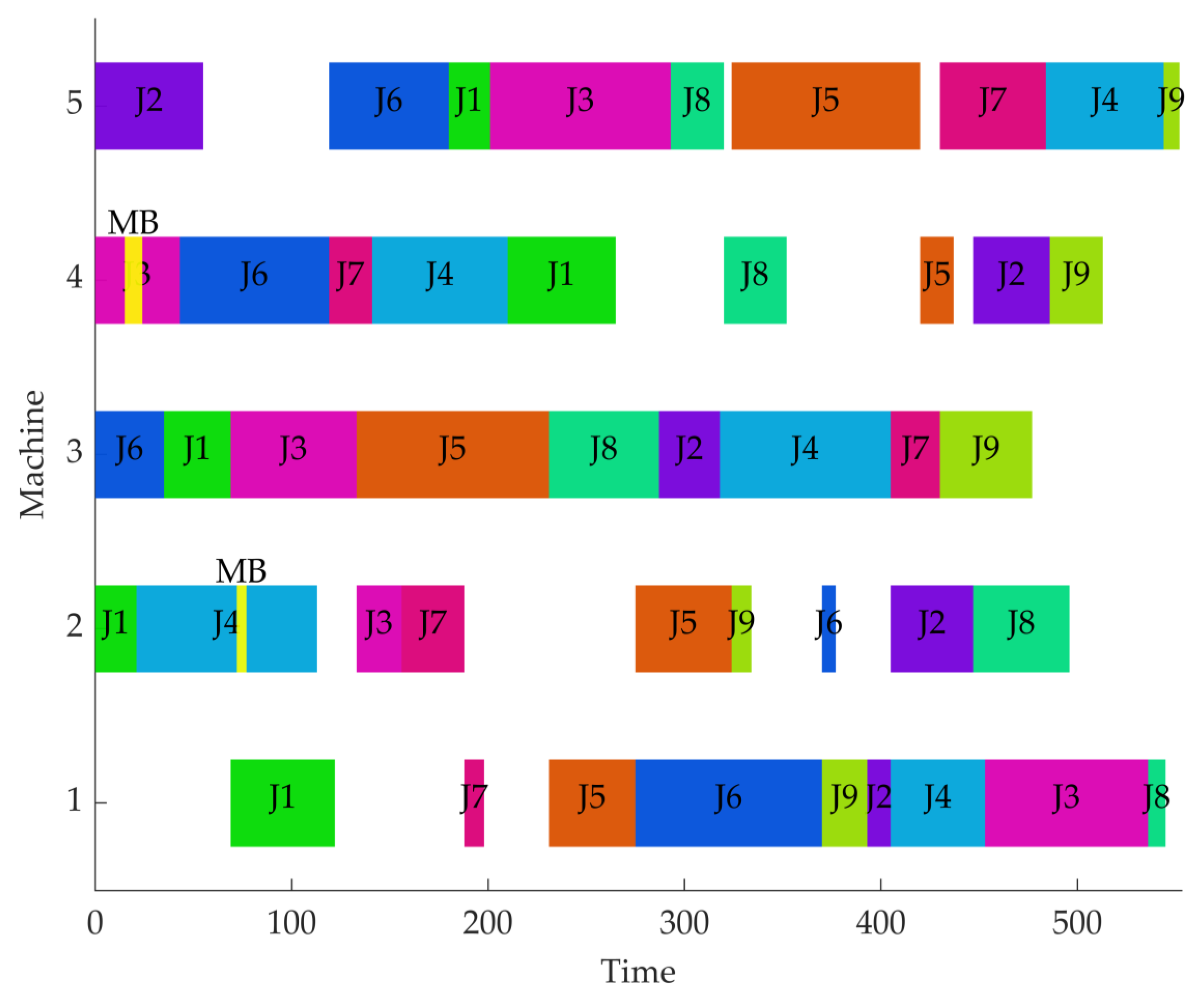
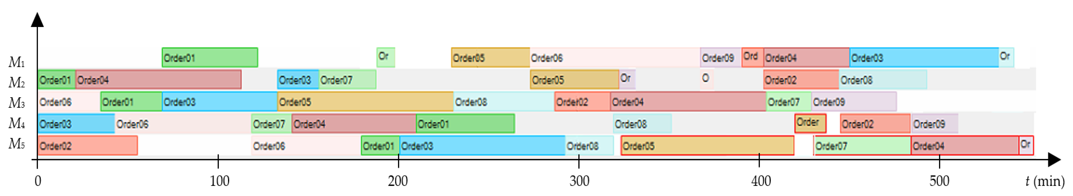
5.2. Simulation Modeling Results

The main purpose of using the simulation model was the data transfer between the numerical results of the optimization IHKA and the real, dynamically changing production system. Given the globally highly competitive environment and the need for a flexible and dynamically fast-responsive production system, a fashion that enables the connection between the decision method and the real environment is crucial.

Table 7. The job’s operation sequence in relation to machine priority number.

		Job’s Sequence
Job priority number		1	2	3	4	5	6	7	8	9
Machine	M1	J1,3	J7,3	J5,2	J6,4	J9,2	J2,3	J4,4	J3,5	J8,5
	M2	J1,1	J4,1	J3,3	J7,2	J5,3	J9,1	J6,5	J2,4	J8,4
	M3	J6,1	J1,2	J3,2	J5,1	J8,1	J2,2	J4,3	J7,4	J9,3
	M4	J3,1	J6,2	J7,1	J4,2	J1,5	J8,3	J5,5	J2,5	J9,4
	M5	J2,1	J6,3	J1,4	J3,4	J8,2	J5,4	J7,5	J4,5	J9,5

shows the job’s sequence according to the assigned machine and the used variable Job Priority Number, which determines the sequence of performing operations on an individual machine specifically. The variable used allows the simulation model to use the optimization data generated by the IHKA. The specifically assigned value of the Job Priority Number variable for an individual operation also defines the dynamic events type (MB, PTC, or NJA) and characteristics that run during the simulation model execution.

Given the limitations of decision algorithms related to the lack of connections with the real-world environment, the proposed simulation model allows the validation of key production system parameters.

Table 8. The machine utilization and process time simulation model results.

Machine	M1	M2	M3	M4	M5	Total Average
Machine utilization (%)	69.2	65.5	100	74.1	85.9	78.9
Machine process time (min)	377	325	477	380	474	406.6

presents the numerical values of the machine utilization parameter and the total process time of an individual machine. The values in the Table prove that the IHKA allows a high degree of scheduling justification from the point of view of high machine utilization, as the average value is 78.9%, which is very high, considering that the data describe job shop production. However, with a high theoretical machine utilization, as shown in the M₃ machine, its performance needs to be evaluated in detail, as such a high theoretical utilization could lead to a bottleneck in the production system. A detailed analysis confirmed, from the graphical results in Figure 7, that the job scheduling performed with the IHKA was able to distribute the optimal schedule, and, thus, allow the smooth operation of the production system. Numerical values of the machine process time parameter prove the adequacy of communication between the IHKA optimization algorithm and the simulation model, as the sums of process times of the simulation model results match the process times assumed in the datasets and terminated by the IHKA.

A detailed analysis of the simulation results evaluates the order flow time. The flow time of the order depends on the time of performing an individual operation on the machine and a dynamic event that can extend or shorten its duration.

Table 9. The order flow time simulation model results and dynamic event job affiliation.

Job	J1	J2	J3	J4	J5	J6	J7	J8	J9	Total Average
Order flow time (min)	265	486	536	523	304	377	365	314	228	377
Dynamic event			MB/PTC	MB/PTC			NJA	NJA	NJA

shows the flow times of orders, and identifies the dynamic events that occurred during model execution. The numerical results prove that the longest order flow times are those in which the dynamic event of an unexpected machine breakdown occurred. This time affected the total order flow time and, consequently, the total average order flow time. It can be found that, in the event of a machine breakdown, it is important to reduce its time to a minimum, if possible, or to adjust the time of performing upcoming operations as shown in the job J₄.

The result of the simulation modeling is a graphical representation of the scheduling of the working tasks of the DJSSP dataset 6 × 5. The Gantt chart in Figure 9 corresponds exactly to the Gantt chart in Figure 8, proving that the presented method of using the optimization results of the IHKA enable communication between the decision algorithm and the real-world environment staged in the simulation environment.

6. Discussion

The IHKA proposed in this paper was applied to solve the 15 benchmark instances of DJSSP. The performance of IHKA is clarified by comparing it with the original HKA and GAM.

First, the results show that both IHKA and HKA performed very well in solving the 15 benchmark instances of DJSSP, and their results were better than GAM [19]. In 30 independent runs of each benchmark instance of DJSSP, they all showed strong robustness. Their robustness of fitness and running time performed very well. Moreover, their running time was very short (less than 30 s even for large size problems), that is, each algorithm can obtain the best solution to the problem in a reasonable time for each instance of DJSSP. It shows that these two algorithms are suitable to solve DJSSP.

The results show that the convergence rate of IHKA was significantly reduced, which helped to avoid the algorithm falling into the local optimum. That is, the introduced cellular neighbor network played an important role. Furthermore, two different cellular neighborhood structures, Von Neumann neighborhood and Moore neighborhood, are used by IHKA. The results show that different cellular neighborhood structures affect the performance of the algorithm. In the 15 benchmark instances of DJSSP, the neighborhood structure of Moore was not as good as Von Neumann. It shows that the cellular neighborhood structure of the cellular neighbor network introduced by IHKA is worthy of further exploration.

According to the proposed integration-communication protocol, Figure 1, a simulation model was built in the conventional Simio simulation environment, made for evaluation of the 6 × 5 DJSSP dataset. The integration-communication protocol allows the use of the scheduling results of the IHKA in the decision logic of the simulation model. The results prove the correspondence of numerical (machine process time, orders’ flow time and makespan) and graphical optimization results (Gantt chart of IHKA and simulation model) with the results of the simulation model. These results prove how important the use of evolutionary computation methods is in solving NP-hard optimization, since the production parameters (machine utilization, orders’ flow time) proved the highly optimized degree of DJSSP scheduling with the IHKA, although dynamic events appeared. The proven successful integration-communication protocol affects significantly the high ability to use the proposed decision-making logic in a real-world production environment, which distinguishes the presented research work, along with a new own IHKA DJSSP decision method, from the research work of other researchers. The use of a conventional simulation tool enables the smooth adaptation of the simulation model structure according to the individually analyzed system, while the proposed decision logic and integration-communication protocol remain sustainably applicable.

Given that the presented research work addresses the DJSSP optimization problem, one of its theoretical limitations is the pre-known sequence of machines assigned to perform individual operations. The transition from single-objective optimization (current state) to DFJSSP, and, thus, to multi-objective decision-making, would enable the elimination of this limitation, which has now been partially eliminated within the simulation model.

7. Conclusions

This paper proposes IHKA by introducing the cellular neighbor network. The cellular neighbor network consists of the best positions experienced by individuals in the population. A boundary constraint handling function is also introduced to enhance the diversity of the population. An encoding method based on relative position index was introduced, so that IHKA can be applied to solve the DJSSP. Both IHKA and HKA were used to solve the 15 benchmark instances of DJSSP, and their performances clarified. The introduction of the cellular neighbor network reduced the convergence rate of HKA. Moreover, the use of multiple cellular neighborhood structures can prevent IHKA from falling into the local optimum. However, further research is needed to improve the performance of IHKA using a cellular neighbor structure.

In conclusion, we find that the newly developed decision-making method allows a satisfactorily good solution for the DJSSP optimization problem. It complements its application usability with an efficient integration-communication protocol, which transfers the optimization results to a conventional simulation environment. A comprehensive treatment of the DJSSP optimization problem allows the application of the proposed methods directly in a real-world production environment.

In the following, it would be useful to evaluate the performance of methods on datasets obtained from real-world production systems, and, thus, examine the capabilities of dynamic decision-making in real-time. Given the limitations of the DJSSP optimization problem, the trend of further research will focus on extending the proposed single-criterion methods to multi-criteria methods (DFJSSP consideration), since then IHKA will also be able to determine machine sequence according to a possible set of machines to perform an individual operation. This development step will contribute to an even higher level of applicability of the proposed method, as, in the real-world environment, decisions are often made as to which machine is the most suitable for and most efficient at performing a specific operation.

References

1. Toscano, R.; Lyonnet, P. A new heuristic approach for non-convex optimization problems. Inf. Sci. 2010, 180, 1955–1966. [Google Scholar] [CrossRef]
2. Adibi, M.A.; Zandieh, M.; Amiri, M. Multi-objective scheduling of dynamic job shop using variable neighborhood search. Expert Syst. Appl. 2010, 37, 282–287. [Google Scholar] [CrossRef]
3. Shahrabi, J.; Adibi, M.A.; Mahootchi, M. A reinforcement learning approach to parameter estimation in dynamic job shop scheduling. Comput. Ind. Eng. 2017, 110, 75–82. [Google Scholar] [CrossRef]
4. Vinod, V.; Sridharan, R. Simulation modeling and analysis of due-date assignment methods and scheduling decision rules in a dynamic job shop production system. Int. J. Prod. Econ. 2011, 129, 127–146. [Google Scholar] [CrossRef]
5. Xiong, H.; Fan, H.; Jiang, G.; Li, G. A simulation-based study of dispatching rules in a dynamic job shop scheduling problem with batch release and extended technical precedence constraints. Eur. J. Oper. Res. 2017, 257, 13–24. [Google Scholar] [CrossRef]
6. Zhang, L.; Gao, L.; Li, X. A hybrid genetic algorithm and tabu search for a multi-objective dynamic job shop scheduling problem. Int. J. Prod. Res. 2013, 51, 3516–3531. [Google Scholar] [CrossRef]
7. Park, J.; Mei, Y.; Nguyen, S.; Chen, G.; Zhang, M. An investigation of ensemble combination schemes for genetic programming based hyper-heuristic approaches to dynamic job shop scheduling. Appl. Soft Comput. 2018, 63, 72–86. [Google Scholar] [CrossRef]
8. Turker, A.K.; Aktepe, A.; Inal, A.F.; Ersoz, O.O.; Das, G.S.; Birgoren, B. A decision support system for dynamic job-shop scheduling using real-time data with simulation. Mathematics 2019, 7, 278. [Google Scholar] [CrossRef] [Green Version]
9. Rajabinasab, A.; Mansour, S. Dynamic flexible job shop scheduling with alternative process plans: An agent-based approach. Int. J. Adv. Manuf. Technol. 2011, 54, 1091–1107. [Google Scholar] [CrossRef]
10. Nie, L.; Gao, L.; Li, P.; Li, X. A GEP-based reactive scheduling policies constructing approach for dynamic flexible job shop scheduling problem with job release dates. J. Intell. Manuf. 2013, 24, 763–774. [Google Scholar] [CrossRef]
11. Geyik, F.; Dosdogru, A.T. Process plan and part routing optimization in a dynamic flexible job shop scheduling environment: An optimization via simulation approach. Neural Comput. Appl. 2013, 23, 1631–1641. [Google Scholar] [CrossRef]
12. Shen, X.-N.; Yao, X. Mathematical modeling and multi-objective evolutionary algorithms applied to dynamic flexible job shop scheduling problems. Inf. Sci. 2015, 298, 198–224. [Google Scholar] [CrossRef] [Green Version]
13. Hosseinabadi, A.A.R.; Siar, H.; Shamshirband, S.; Shojafar, M.; Nasir, M.H.N.M. Using the gravitational emulation local search algorithm to solve the multi-objective flexible dynamic job shop scheduling problem in small and medium Enterprises. Ann. Oper. Res. 2015, 229, 451–474. [Google Scholar] [CrossRef]
14. Gocken, T.; Dosdogru, A.T.; Boru, A.; Gocken, M. Integrating process plan and part routing using optimization via simulation approach. Int. J. Simul. Model. 2019, 18, 254–266. [Google Scholar] [CrossRef]
15. Yu, M.R.; Yang, B.; Chen, Y. Dynamic integration of process planning and scheduling using a discrete particle swarm optimization algorithm. Adv. Prod. Eng. Manag. 2018, 13, 279–296. [Google Scholar] [CrossRef] [Green Version]
16. Ren, T.; Zhang, Y.; Cheng, S.-R.; Wu, C.-C.; Zhang, M.; Chang, B.; Wang, X.; Zhao, P. Effective heuristic algorithms solving the jobshop scheduling problem with release dates. Mathematics 2020, 8, 1221. [Google Scholar] [CrossRef]
17. Zhang, H.; Zhang, Y.Q. A discrete job-shop scheduling algorithm based on improved genetic algorithm. Int. J. Simul. Model. 2020, 19, 517–528. [Google Scholar] [CrossRef]
18. Ojstersek, R.; Zhang, H.; Liu, S.; Buchmeister, B. Improved heuristic Kalman algorithm for solving multi-objective flexible job shop scheduling problem. Procedia Manuf. 2018, 17, 895–902. [Google Scholar] [CrossRef]
19. Kundakcı, N.; Kulak, O. Hybrid genetic algorithms for minimizing makespan in dynamic job shop scheduling problem. Comput. Ind. Eng. 2016, 96, 31–51. [Google Scholar] [CrossRef]
20. Toscano, R.; Lyonnet, P. A kalman optimization approach for solving some industrial electronics problems. IEEE Trans. Ind. Electron. 2012, 59, 4456–4464. [Google Scholar] [CrossRef]
21. Zhang, H.; Buchmeister, B.; Liu, S.; Ojstersek, R. Use of a simulation environment and metaheuristic algorithm for human resource management in a cyber-physical system. In Simulation for Industry 4.0; Gunal, M., Ed.; Springer: Cham, Germany, 2019; pp. 219–246. [Google Scholar] [CrossRef] [Green Version]
22. Li, X.; Li, X.; Yang, L.; Li, J. Dynamic route and departure time choice model based on self-adaptive reference point and reinforcement learning. Phys. A Stat. Mech. its Appl. 2018, 502, 77–92. [Google Scholar] [CrossRef]
23. Von Neumann Neighborhood. Available online: https://en.wikipedia.org/wiki/Von_Neumann_neighborhood (accessed on 26 August 2020).
24. Moore Neighborhood. Available online: https://en.wikipedia.org/wiki/Moore_neighborhood (accessed on 16 December 2020).
25. Marinakis, Y.; Marinaki, M. A hybrid particle swarm optimization algorithm for the open vehicle routing problem. In Swarm Intelligence. ANTS 2012. Lecture Notes in Computer Science; Dorigo, M., Birattari, M., Blum, C., Christensen, A.L., Engelbrecht, A.P., Groß, R., Stützle, T., Eds.; Springer: Berlin, Germany, 2012; pp. 180–187. [Google Scholar] [CrossRef]
26. Milgram, S. The small world problem. Psychol. Today 1967, 1, 60–67. [Google Scholar]
27. Ojstersek, R.; Lalic, D.; Buchmeister, B. A new method for mathematical and simulation modelling interactivity: A case study in flexible job shop scheduling. Adv. Prod. Eng. Manag. 2019, 14, 435–448. [Google Scholar] [CrossRef]
Figure 1. The proposed integration-communication protocol.
Mathematics 09 00909 g001
Figure 2. The flowchart of the HKA.
Mathematics 09 00909 g002
Figure 3. The flowchart of the IHKA.
Mathematics 09 00909 g003
Figure 4. The instances of cellular neighborhood and cellular neighbor network.
Mathematics 09 00909 g004
Figure 5. The instance of the solution encoding.
Mathematics 09 00909 g005
Figure 6. The simulation model in Simio.
Mathematics 09 00909 g006
Figure 7. The IHKA and HKA average convergences of the best solutions for the benchmark instances of DJSSP (the horizontal line is the fitness of the best solution obtained by GAM for each instance).
Mathematics 09 00909 g007
Figure 8. The Gantt chart of the 6 × 5 DJSSP with IHKA VonNeumann.
Mathematics 09 00909 g008
Figure 9. The Gantt chart of the 6 × 5 DJSSP with IHKA VonNeumann results obtained in Simio.
Mathematics 09 00909 g009