Article

μ-Synthesis for Fractional-Order Robust Controllers

Department of Automation, Technical University of Cluj-Napoca, Str. G. Bariţiu nr. 26-28, 400027 Cluj-Napoca, Romania
*
Authors to whom correspondence should be addressed.
These authors contributed equally to this work.
Mathematics 2021, 9(8), 911; https://doi.org/10.3390/math9080911
Submission received: 28 February 2021 / Revised: 12 April 2021 / Accepted: 16 April 2021 / Published: 20 April 2021
(This article belongs to the Special Issue Applications of Mathematical Models in Engineering)

Abstract

:
The current article presents a design procedure for obtaining robust multiple-input and multiple-output (MIMO) fractional-order controllers using a μ -synthesis design procedure with DK iteration. μ -synthesis uses the generalized Robust Control framework in order to find a controller which meets the stability and performance criteria for a family of plants. Because this control problem is NP-hard, it is usually solved using an approximation, the most common being the DK iteration algorithm, but, this approximation leads to high-order controllers, which are not practically feasible. If a desired structure is imposed to the controller, the corresponding K step is a non-convex problem. The novelty of the paper consists in an artificial bee colony swarm optimization approach to compute the nearly optimal controller parameters. Further, a mixed-sensitivity μ -synthesis control problem is solved with the proposed approach for a two-axis Computer Numerical Control (CNC) machine benchmark problem. The resulting controller using the described algorithm manages to ensure, with mathematical guarantee, both robust stability and robust performance, while the high-order controller obtained with the classical μ -synthesis approach in MATLAB does not offer this.

1. Introduction

One of the active problems with major impact which have been studied for years in Control Theory refers to robustness. Robustness encompasses the sensitivity of a control system with respect to both internal and external disturbances. Several robust methods have been developed in order to achieve robust performance and stability in the presence of uncertainties. Robust control problems use H 2 and H norms defined in frequency domain as a performance measure. To solve H 2 / H control problems, there are several approaches. One possible solution is presented in [1] and is based on Algebraic Riccati Equations (AREs). A more numerically stable approach to solve ARE was developed using Popov triplets in [2], approach recently implemented in an open-source manner in [3], with an iterative refinement method presented in [4], but an ARE-based solution presents a limitation due to the impossibility of solving singular problems. An alternative way which manages to solve such problems was introduced in [5], where AREs were replaced by Algebraic Riccati Inequalities (ARIs). ARIs are solved through Linear Matrix Inequalities (LMIs), while regular assumptions are no longer needed due to LMI system versatility. An open-source solver for Robust Control problems using LMIs is presented in [6].
The H 2 / H approach designs a suitable controller for the nominal plant, therefore only nominal stability and nominal performance are fulfilled. Additionally, generalized Robust Control framework allows to impose robust stability and robust performance, which cover the previous two aspects for an entire family of physical processes. As such, the  μ -synthesis approach extends the H optimization in order to obtain a robust controller for the uncertain plant which includes parametric and dynamic uncertainties [7,8]. μ -synthesis is based on using structured singular values to quantify robustness margins and also on using linear fractional descriptions of the control problem containing the nominal plant model and uncertainty weighting functions. In [9], the authors present the μ -synthesis problem used with the so-called DK iteration, which, in essence, provides two steps iteratively repeated until the robust performance stops improving: designing a H control law and μ analysis on closed-loop system.
μ -synthesis is, however, a non-convex problem and the DK iteration represents only an approximation, without any convergence guarantees. Another significant concern of DK iteration is that the method generates high order controllers. In order to solve this issue, various approaches based on fixed structure controller are proposed in different papers [10,11,12]. The method presented in [10] uses nonsmooth techniques for H synthesis. Then, using the same technique, the  μ -synthesis was solved using DK iteration and the result are presented in [13].
The main issue which appears when controller structure constraints are imposed is that the optimization problem in no longer convex and also, μ -synthesis is in general, considered nondeterministic polynomial time hard (NP-hard). A possible solution to that are swarm optimization algorithms. There are different approaches presented in papers [14,15,16] based on Genetic Algorithms (GA) and Particle Swarm Optimization (PSO). A solution for imposing a fixed structure controller, such as low-order or decentralized, was proposed in paper [14], which splits the problem in two parts: the convex part, solved using the classical ARE approach, and the non-convex part, solved using GA. The same authors proposed in [16] a new technique based on an evolutionary D K D 0 iteration method, which combines the classical D-step with a K D 0 algorithm based on also a GA. Authors of the paper [15] propose an evolutionary approach to solve the μ -synthesis problem without order reduction by using an improved PSO.
Artificial Bee Colony (ABC) can also be used to solve complex optimization problems with constraints and could possibly outperform the other approaches and return the best solution in shorter execution time. The initial idea was presented in [17] as an extension of another metaheuristic algorithm, namely Honey Bee Swarm (HBS). The efficiency of the algorithm for several state-of-the-art optimization problems, along with an improvement for the stopping criterion, were underlined in [18].
One possible fixed structure controller is fractional-order proportional-integral-derivative (FO-PID). FO-PID is one of the most remarkable fractional order techniques with great interest in research [19]. It is used to generalize the classical PID control by adding extra degrees of freedom [20]. Compared to the integer PID controller, FO-PID brings the advantage of improving the robustness and providing better performance. In [21], the authors propose a FO-PID controller for a fractional-order plant model, presenting an analysis in both frequency and time domains, proving that achieving better control performance is one of the advantages of this approach. The FO-PID was used on a benchmark problem, i.e., the speed control of a DC motor [22], obtaining good results in terms of performance and robustness. Two generalized versions of Kessler’s magnitude method with fractional order controllers were developed in [23,24]. A detailed comparison between classical modelling approaches and a fractional integrator approximation as a control baseline model is presented to the servo problem in [25]. A graphical method was developed in [26], while in [27] a fractional order internal model controller with event-based implementation was developed. Other applications comprise in an optimal FO-PID controller for a PMSM speed control, presented in [28], while a robust controller for a steam turbine was developed in [29].
In this paper, we present a new technique to design FO-PID robust controllers using μ -synthesis. The novelty of the current approach consists in implementing an algorithm able to find the nearly optimal values of the controller parameters using an artificial bee colony optimization. The cost function to be minimized is the H norm of the closed-loop system, when stable, and, otherwise, a large value affinely dependent on the largest real part of the eigenvalues of the closed-loop state matrix. Therefore, the non-convex part of the NP-hard μ -synthesis problem is solved using such a swarm optimization, while the D step is solved using the classical LMI technique. More than that, the realp object from MATLAB’s Robust Control Toolbox embodies a limitation because it cannot be used as an exponent, necessary in approximating the fractional element with an integer-order system. Our approach manages to deal with this limitation in order to obtain the controller parameters, because the only information necessary in our approach is the range of the controller’s parameters stored in such variables, which can be replaced with a simpler software object. Additionally, using our approach, a numerical example illustrates that the resulting controller manages to fulfill the robust stability and performance, while the controller obtained using unstructured μ -synthesis does not rigorously guarantee these specifications. Therefore, our method proposes a general framework able to synthesize arbitrary fixed structure fractional order controllers by optimizing their parameters in terms of robustness and performance, surpassing the well-established approach of manually tuning them for a desired problem, harnessing the Robust Control framework’s design strongness.
We illustrate our proposed method on a benchmark problem: obtaining a controller for a two axis computer numerical control (CNC) system by solving a mixed-sensitivity μ -synthesis problem. Several control methods using the state space model of the machine are presented in literature. A comparison between the classical pole-placement method and Linear Quadratic Regulator (LQR) method is presented in [30]. For the LQR problem, an energy-based minimization algorithm was proposed, which proves to be suitable in terms of stability and robustness. As presented in [31], a different approach is recommended, in order to obtain a PI controller for each axis, using the state-feedback control algorithm. In this case, the state space model is augmented with an extra state which represents the integral of the position. The PI regulator parameters are obtained from the state-feedback gains.
The paper is organized in four sections. Section 2 introduces several ideas relevant to the proposed method, such as a mathematical foundation of FO-PID, continuing with the fundamental robust control problem based on μ -synthesis, and, finally, the ABC optimization algorithm. After that, the last subsection focuses on solving the non-convex problem of computing fixed structure controllers. Section 3 illustrates an application of the proposed method for position control of a two axis CNC machine, along with numerical results. In Section 4, the previously mentioned results are compared with those obtained using the well-established algorithms from MATLAB. Finally, conclusions are presented in Section 5.

2. Materials and Methods

In this section we present a controller synthesis procedure which manages to find a fixed structure fractional-order controller using the μ -synthesis technique from the Robust Control framework, where the non-convex subproblem involved in the classical DK iteration is replaced by a swarm optimization algorithm. First, the mathematical background comprised in fractional-order control, robust control and artificial bee colony optimization is underlined, while the fourth subsection presents the proposed design procedure using all the mechanisms briefly described.

2.1. Fractional-Order Controller

The classical integer-order calculus was extended by Riemann and Liouville to fractional-order calculus by introducing the fractional integral operator [32]:
I a α f ( t ) = 1 Γ ( α ) a t f ( τ ) ( t τ ) α 1 d τ ,
where Γ ( α ) : C + C is the Euler Gamma function and the order of the integral operator is the complex parameter α C + . This extension develops a new area of research in the Control System domain. A commonly used definition of this operator was introduced in [33] as:
J C α f ( t ) = 1 Γ ( α ) 0 t ( t τ ) α 1 f ( τ ) d τ = I 0 α f ( t ) ,
with t > 0 and α R + , having the Laplace transform [34]:
L { J c α f ( t ) } ( s ) = s α F ( s ) ,
where F ( s ) = L f ( t ) ( s ) . One of the most common controller structures used in practice is the proportional-integral-derivative (PID) controller, having three degrees of freedom. Using fractional-order calculus, two new degrees of freedom can be added to a PID, having the notation PIλDμ. As such, the fractional order PID (FO-PID) has, as extra degrees of freedom, the order λ R + of the integrator and the order μ R + of the differentiator, with the resulting transfer function:
H c ( s ) = K P + K I s λ + K D s μ .
The time domain expression of the command signal c ( t ) can be expressed using the error signal ε ( t ) as:
c ( t ) = K p · ε ( t ) + K I · J c λ { ε ( t ) } + K D · J c μ { ε ( t ) } .
One of the major issues of such a fractional element, i.e.,  J c λ or J c μ , is its implementation. In order to solve this problem, the Oustaloup recursive approximation (ORA) was introduced [35], and allows the approximation of the fractional-order element with an LTI system of pre-specified order N:
s λ = k = 1 N 1 + s / ω z , k 1 + s / ω p , k ,
where the frequency values of the singularities are obtained based on the desired fractional order λ ( 0 , 1 ) , the integer order of the approximation N, along with the frequency range in which the approximation is valid [ ω l , ω u ] . Using the following two coefficients:
ε = ω u ω l λ N and η = ω u ω l 1 λ N ,
the above mentioned frequencies can be computed using:
ω z , 1 = ω l η ,
ω p , n = ω z , n · ε , n = 1 , N ¯ ,
ω z , n + 1 = ω p , n · η , n = 1 , N 1 ¯ .
For the rest of the possible real values of λ , the approximation can be easily extended as: for λ ( 1 , 0 ) by inverting the relation (6), while for | λ | 1 , the components could be the integer part [ λ ] and the fractional part { λ } , with the fractional part only approximated using (6).

2.2. Robust Control

The Robust Control framework assumes to minimize the H 2 / H norm of the lower linear fractional transformation (LLFT) of a plant P and a controller K:
P o = LLFT ( P , K ) = P 11 + P 12 K ( I P 22 K ) 1 P 21 ,
where the plant P can be written, in general form, as:
P : P 11 P 12 P 21 P 22 = A B w B u C z D z w D z u C y D y w D y u ,
where the signals involved in the above relation will be further detailed in a more general context. One approach to solving H 2 / H problems is using AREs, which presents several limitations that are removed by the LMI approach. However, this framework can be used to ensure nominal stability and nominal performance only, but, the plant P must also contain an augmented model of the real process in which uncertainties are also present. There are two classic uncertainties types: parametric, represented by δ I , where δ is the maximum bound of the parameter for a physical variable, and unstructured, represented by a full block Δ R m × m . The latter illustrates neglected or unknown dynamics uncertainties. In the mixed-scenario case, the following set is considered:
Δ = Δ = diag δ 1 I n 1 , , δ s I n s , Δ 1 , , Δ f | δ k R , Δ j R m j × m j , k = 1 , s ¯ , j = 1 , f ¯ .
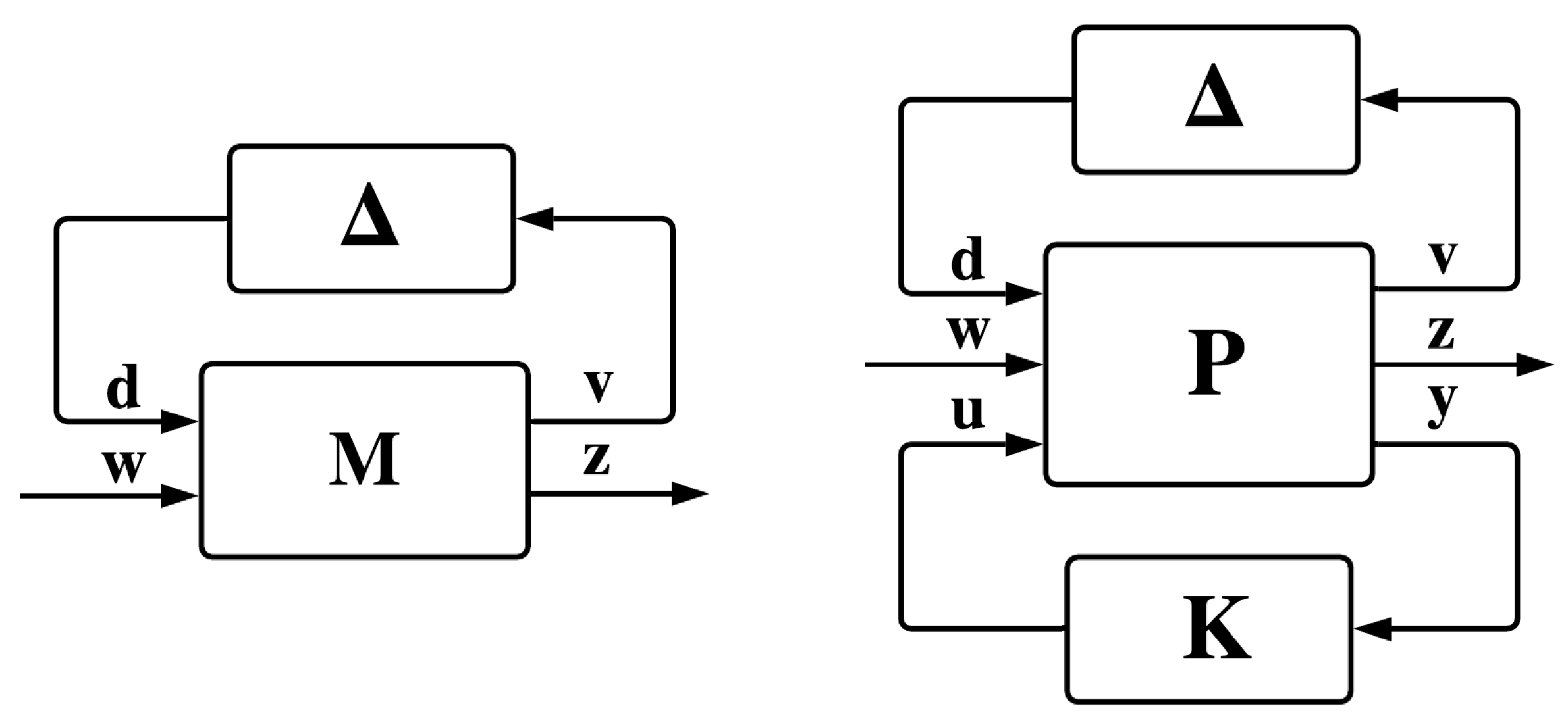
In the Robust Control field, one of the main tools used for robustness analysis is the structured singular value, defined as follows.
Definition 1.
For a square matrix M C N × N the structured singular value with respect to the set Δ is:
μ Δ ( M ) = 1 min Δ Δ { σ ¯ ( Δ ) | det ( I M Δ ) = 0 } ,
if there exists Δ Δ such that the matrix I M Δ is rank deficient, otherwise 0.
For an LTI system described by the transfer matrix M ( s ) and an upper linear fractional transformation (ULFT) connection shown in Figure 1 (left), the structured singular value μ Δ ( M ) can be defined as:
μ Δ ( M ( s ) ) = sup ω R + μ Δ ( M ( j ω ) ) .
Now, considering M ( s ) = LLFT ( P , K ) ( s ) as being the lower linear fractional transformation (LLFT) between plant P and controller K, the connection illustrated in Figure 1 (right) results. The generalized plant structure is:
P Δ ( s ) = P v d ( s ) P v w ( s ) P v u ( s ) P z d ( s ) P z w ( s ) P z u ( s ) P y d ( s ) P y w ( s ) P y u ( s ) P Δ : x ˙ ( t ) v ( t ) z ( t ) y ( t ) = A B d B w B u C v D v d D v w D v u C z D z d D z w D z u C y D y d D y w D y u x ( t ) d ( t ) w ( t ) u ( t ) ,
where three types of input signals are present—the command input u R n u , the performance input w R n w , and the disturbance input d R n d —and three types of outputs—the measurements vector y R n y , the performances vector z R n z , and the disturbance output v R n v .
Besides the well-known H 2 / H methods, a controller that meets robust stability and robust performance alike can be computed using the μ -synthesis framework. Robust stability implies that a specific controller manages to stabilize all the processes described by the upper linear fractional transformation (ULFT) presented in Figure 1 (left), while robust performance implies that the controller is able to impose the desired closed-loop performance in the worst case scenario. In order to have a mathematical guarantee that a controller K meets the robust stability and performance, the Main Loop theorem can be used. It implies that closed-loop system meets robust stability and performance if and only if the structural singular value of the LLFT of the plant and controller, with respect to Δ , fulfills:
sup ω R + μ Δ ( LLFT ( P , K ) ( j ω ) ) < 1 .
Therefore, the robust control problem can be written as:
inf K stab . sup ω R + μ Δ ( LLFT ( P , K ) ( j ω ) ) ,
which is not convex. More than that, the structural singular values are hard to be explicitly computed. In practice, there are various bounds which can be used to approximate the structural singular value. One of the most used approximations of the upper bound is in [9]:
μ Δ ( M ) inf D D σ ¯ ( D M D 1 ) ,
where σ ¯ denotes the largest singular value, and the set D is defined as:
D = diag D 1 , , D s , d 1 I m 1 , , d f I m f | D k = D k R n k × n k , d j > 0 , k = 1 , s ¯ , j = 1 , f ¯ .
Based on this upper bound, a good approximation of the initial non-convex problem can be employed by solving the following quasi-convex problem:
inf K stab . sup ω R + inf D D σ ¯ D ( j ω ) · LLFT ( P , K ) ( j ω ) · ( D ( j ω ) ) 1 .
If the scaling factor, represented by the system D, is fixed, then the problem (21) is nothing but a H optimization problem. On the other hand, fixing the controller K, the D scaling step can now be obtained by solving a Parrot problem for a desired frequency set Ω = { ω 1 , , ω N } using the following generalized eigenvalue problem:
min γ , s . t . LLFT ( P , K ) ( j ω i ) * · X · LLFT ( P , K ) ( j ω i ) γ 2 X ,
where from the solution X = D ( j ω i ) * · D ( j ω i ) , the matrix D ( j ω i ) can be extracted using a singular value decomposition. After all Parrot problems are solved, a minimum phase system is found in order to approximate the analytical solution D ( s ) . In summary, an iterative algorithm which solves the μ -synthesis problem starts by setting D = I , with the following steps applied successively:
1: 
Fix D and solve the H optimal problem to find a controller K:
K = arg inf K stab . | | LLFT ( P , K ) | | .
2: 
Fix the controller K and solve the set of convex problems:
D ( j ω ) = arg inf D D σ ¯ D · LLFT ( P , K ) ( j ω ) · D 1 ,
for a given frequency range Ω and, then, fit a stable minimum phase transfer matrix D ( s ) .
Steps 1 and 2 are executed in a loop sequence until the difference between two consecutive H norms is less than a prescribed tolerance or the maximum number of iterations is reached.

2.3. Artificial Bee Colony Optimization

The artificial bee colony (ABC) optimization is a nature-inspired algorithm used to minimize a cost function:
f : D R , where D = [ l b 1 , u b 1 ] × [ l b 2 , u b 2 ] × × [ l b d , u b d ] R d .
The ABC algorithm mimics the behaviour of real honeybees, where each food source represents a possible solution of the optimization problem described above. The location and the amount of nectar correspond to the design variables and the cost function, respectively. The bees are divided in two main groups: employed and unemployed bees, while the unemployed bees could be of two types as well: onlooker and scout bees. The employed bees are the ones that investigate the food source and return to the hive to inform the others by performing the waggle dance; the onlooker bees are the ones that watch the dance and decide whether or not a food source is worthy of being searched or not; the scout bees are former employed bees that have abandoned their previous food source, due to lack of nectar, and which now search for a new one. The Best Solution is represented by the food source, and the quality (or cost) of the solution is represented by the amount of nectar.
The number of employed bees coincides with number of the onlooker bees and represents the dimension of the swarm problem, denoted by N. The employed bees start the foraging process by randomly searching an initial position x i ( 0 ) in the domain D:
x i ( 0 ) = l b 1 + ϕ i , 1 ( 0 ) · ( u b 1 l b 1 ) l b 2 + ϕ i , 2 ( 0 ) · ( u b 2 l b 2 ) l b d + ϕ i , d ( 0 ) · ( u b d l b d ) D ,
where ϕ i , 1 , d ¯ ( 0 ) [ 1 , 1 ] are random numbers. After this initialization step, the first Best Solution appears.
Each employed bee searches a new food source based on the location of the current food source x i ( k ) and another food source x j ( k ) randomly selected. The new possible position is:
x ¯ i ( k ) = sat x i ( k ) + ϕ ( x i ( k ) x j ( k ) ) ,
where ϕ [ 1 , 1 ] d is an array of random numbers, ⊙ is the element-wise multiplication, and sat is the saturation function that does not allow the position to be outside the searching domain D. Now, the position of the ith employed bee for the next iteration will be:
x i ( k + 1 ) = arg min { f ( x i ( k ) ) , f ( x ¯ i ( k ) ) } ,
which means that an employed bee will never choose a source with less nectar. If the position for the next iteration will not be changed, the abandonment counter of the ith employed bee increments.
The onlooker bees use the information shared by each employed bee and choose a location around the position of the employed bees. The fitness value of a solution x i ( k ) is given by:
log W ( i ) = f ( x i ( k ) ) 1 N j f ( x j ( k ) ) ,
and the probability that ith bee’s source will be selected by an onlooker bee is:
p i = W ( i ) j W ( j ) .
Now, using a roulette wheel selection method, the onlooker bee will choose a source i and, using the same searching technique as an employed bee, a new position is computed using (27). If the outlooker bee founds a better solution than the ith employed bee, they change their roles, otherwise the abandonment counter for the ith source increments. After this step, we have N employed bees and N unemployed bees. However, if the abandonment counter for the ith source exceeds a threshold, the ith employed bee becomes a scout and tries to find a new location using the relation (26).
After every loop corresponding to employed, outlooker and scout bees, it is checked if there is a food source with a solution better than the last one. The algorithm is over when the maximum number of cycles is reached or when there is no improvement of the Best Solution after a prescribed number of cycles.

2.4. Proposed Method

The solution of the problem described in (21) using the classical DK iteration with H 2 / H framework leads to a high-order controller. As a solution to this issue, a fixed structure family of controllers K can be considered, and the problem (21) becomes:
inf K K K stab sup ω R + inf D D σ ¯ D ( j ω ) · LLFT ( P , K ) ( j ω ) · ( D ( j ω ) ) 1 .
The new problem has the disadvantage of being non-convex in terms of the parameters of the proposed controller structure. However, the problem described in (31) will also be solved using a DK iterative procedure, but the non-convex part of the problem has fewer degrees of freedom and it will be managed with an ABC optimization.
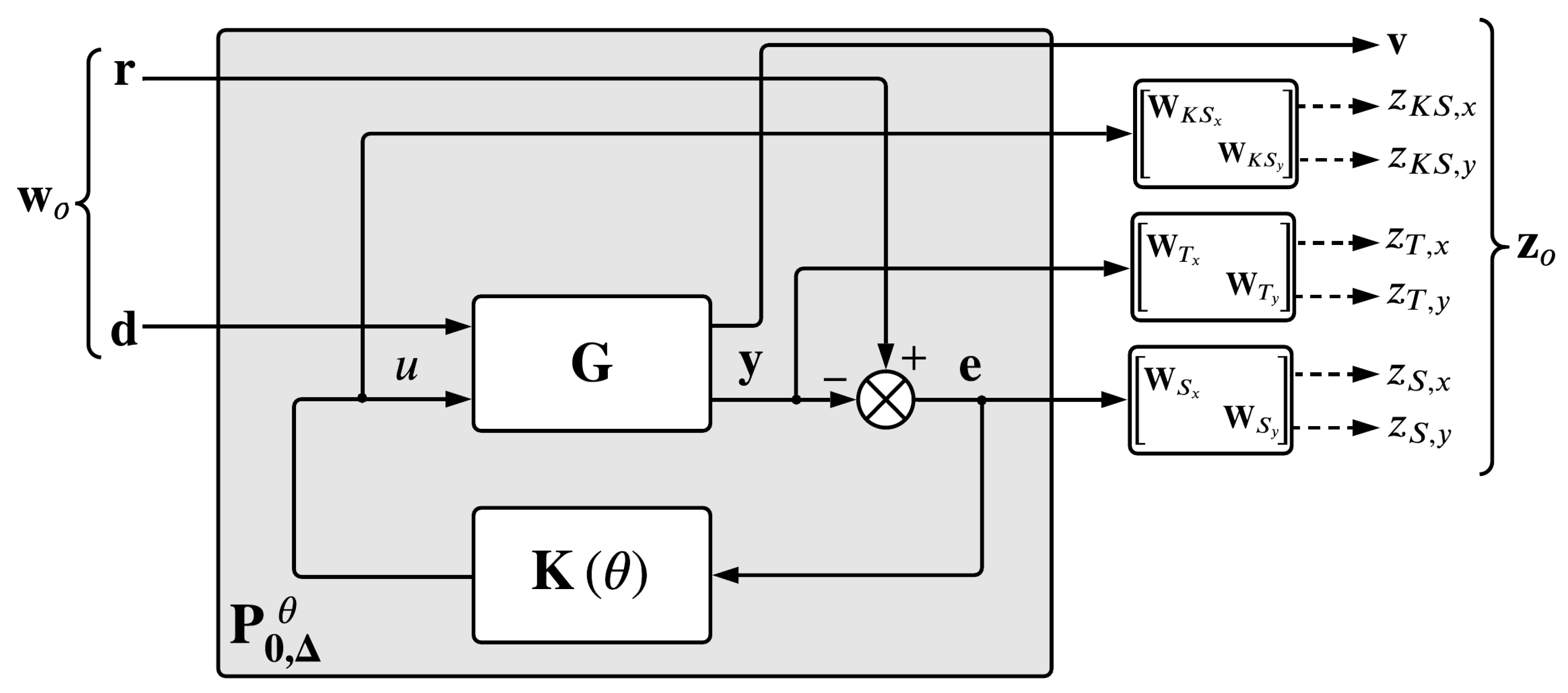
Starting with the model of the process G, a plant P is obtained after the augmentation step:
P : x ˙ ( t ) z ( t ) y ( t ) = A B w B u C z D z w D z u C y D y w D y u x ( t ) w ( t ) u ( t ) ,
where the meaning of the inputs and outputs remains the same as in Section 2.2. Considering the advantages of the fractional-order controllers, the proposed structure of the controller is:
K θ ( s ) = C F O ( 1 , 1 ) ( s ) C F O ( 1 , 2 ) ( s ) C F O ( 1 , n y ) ( s ) C F O ( 2 , 1 ) ( s ) C F O ( 2 , 2 ) ( s ) C F O ( 2 , n y ) ( s ) C F O ( n u , 1 ) ( s ) C F O ( n u , 2 ) ( s ) C F O ( n u , n y ) ( s ) ,
where C F O ( i , j ) is a fractional order controller from the ith input to the jth output and has the form:
C F O ( i , j ) ( s ) = K P ( i , j ) + K i ( i , j ) s λ ( i , j ) + K D ( i , j ) s μ ( i , j ) ,
with the tunable parameters described by the vector:
θ ( i , j ) = K P ( i , j ) K i ( i , j ) λ ( i , j ) K D ( i , j ) μ ( i , j ) D A B C ( i , j ) R 5 .
Using these considerations, the desired family of the fixed structure controllers can be described as follows:
K = K θ ( s ) θ D A B C D A B C ( 1 , 1 ) × D A B C ( 1 , 2 ) × × D A B C ( n u , n y ) ,
where all parameters are stored in a single vector θ describing all degrees of freedom of the tunable controller. Using the ORA mechanism, each component K θ ( s ) K has a state-space representation:
K θ : x ˙ K ( t ) u ( t ) = A K ( θ ) B K ( θ ) C K ( θ ) D K ( θ ) x K ( t ) y ( t )
Next, we denote by P o θ the closed-loop system represented by the lower linear fractional transformation between the augmented plant P and controller K θ , which can be represented as:
P o θ = LLFT ( P , K θ ) : x ˙ o ( t ) z o ( t ) = A o ( θ ) B o ( θ ) C o ( θ ) D o ( θ ) x o ( t ) w o ( t ) ,
where state vector, input vector and output vector of the closed-loop system are:
x o = x x K , w o w and z o z .
In Algorithm 1 the main steps necessary to obtain the parameters of the controller having the structure (33) are presented. The inputs of the algorithm are the closed-loop plant P o θ , containing the tunable controller parameters θ , and the parameters α and β which describe the cost function that needs to be minimized using an ABC optimization, but, P o θ must also contain the varying parameters and unmodelled dynamics. Therefore, the plant P Δ obtained after the augmentation step with uncertainties Δ has the form presented in (16). Thus, the first step made in Algorithm 1 consists in transforming the closed-loop system P o θ in the generalized closed-loop system P o , Δ θ described as follows:
P o , Δ θ = LLFT ( P Δ , K θ ) : x ˙ o ( t ) z ¯ o ( t ) = A ¯ o ( θ ) B ¯ o ( θ ) C ¯ o ( θ ) D ¯ o ( θ ) x o ( t ) w ¯ o ( t ) ,
where the new extended performance inputs and outputs are:
w ¯ o = d w o z ¯ o = v z o
As mentioned in Section 2.2, the structured singular value can be bounded using two D-scaling factors, one for the left and one for the right scaling, denoted D L and D R 
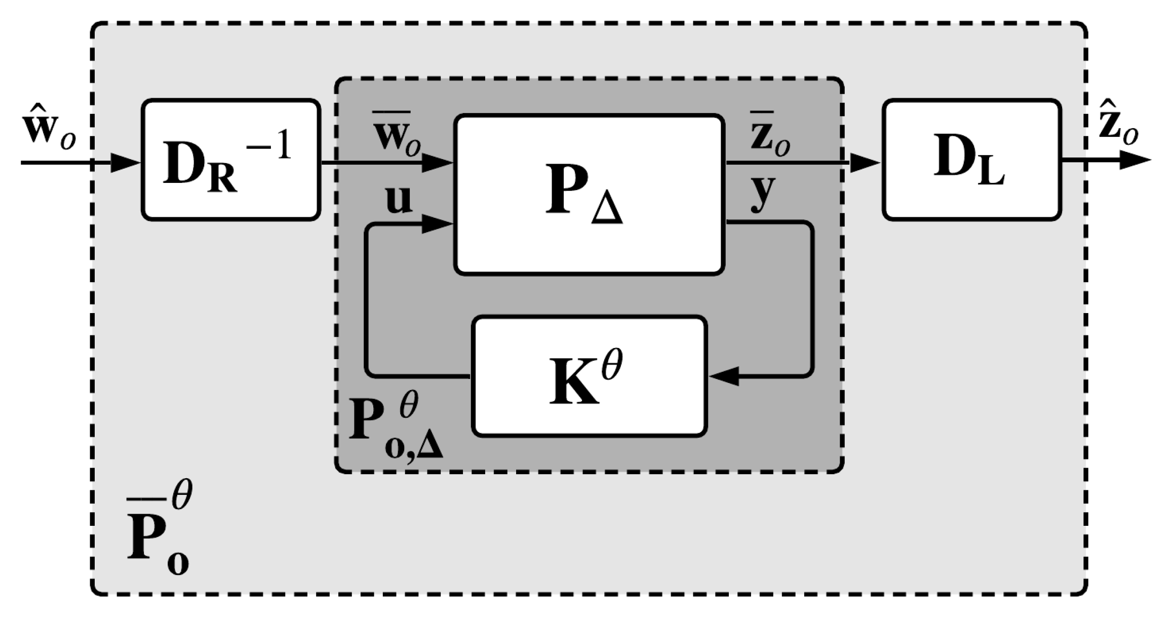
, respectively. As it can be notice in Figure 2, a new closed-loop plant P ¯ o θ is obtained:
P ¯ o ( θ ) ( s ) = D L ( s ) · P o , Δ θ ( s ) · D R 1 ( s ) ,
having the state-space representation:
P ¯ o θ : x ^ ˙ o ( t ) z ^ o ( t ) = A ^ o ( θ ) B ^ o ( θ ) C ^ o ( θ ) D ^ o ( θ ) x ^ o ( t ) w ^ o ( t ) .
All the above mentioned plants are presented in Figure 2. First, the generalized plant P Δ has a LLFT connection with the controller K θ , resulting the closed-loop plant P o , Δ θ , having the input vector w ¯ o and the output vector z ¯ o . After the D-scaling step, a new plant P ¯ o θ is obtained, having the input vector w ^ o and the output vector z ^ o .
Before starting the while loop of Algorithm 1, an initialization of the generalized closed-loop plant with D-scale P ¯ o θ is performed with the initial scale factors D L = I n w and D R = I n z , as seen in line 2. As noticed in line 4, the K step is performed using this generalized plant having as degrees of freedom the tunable parameters θ . In order to compute the controller parameters θ * , the ABC optimization will be used. The cost function to be minimized is:
f : D A B C R + , f ( θ ) = | | P ¯ o θ | | , if P ¯ o θ is stable α λ m a x ( A ^ o ) + β , if P ¯ o θ is unstable ,
where the operator λ m a x is defined by:
λ m a x : R M × M R , λ m a x ( A ) = max { Re ( λ ) | λ Λ ( A ) } .
Algorithm 1: Fixed Structure μ -Synthesis.
Mathematics 09 00911 i001
The procedure computeKstep used to obtain the controller parameters is briefly presented in Algorithm 2 and will be described below. The inputs of the algorithm are the generalized closed-loop plant with D-scaling step P ¯ o θ , along with the parameters α and β which describe the cost function (44). The first step of this routine consists in computing the domain D A B C of the cost function based on the constraints of the tunable parameters. The main limitation is represented by the fractional orders of the integral and derivative effects of the controller which must remain in ( 0 , 1 ) , according to ORA.
In the second step of routine Algorithm 2, an initial population is created. Let N be the dimension of the swarm problem. This parameter can be given as input, but as a good practice, this can be chosen 100 times larger than the number of tunable parameters. The initialization step consists in randomly generating the positions θ 1 ( 0 ) , θ 2 ( 0 ) , , θ N ( 0 ) of the food sources for each employed bee in the domain D A B C using relation (26). After the initialization step, the first Best Solution (BS) is computed as:
θ = arg min f ( θ i ( k ) ) i = 1 , N ¯ B S = f ( θ ) .
Using this initial population, the main while loop starts. In line 4, the employed bees step is performed. In this step, each employed bee searches a new position around using relation (27), resulting N new possible positions for the next step, denoted by θ ¯ 1 ( k ) , θ ¯ 2 ( k ) , , θ ¯ N ( k ) , and the proposed positions of the employed bees at step k + 1 will be:
θ ^ i ( k + 1 ) = arg min { f ( θ i ( k ) ) , f ( θ ¯ i ( k ) ) } , i = 1 , N ¯ .
If, for a specific food source i, the proposed position coincides with the previous position, the abandonment counter increments.
Using the proposed solutions of the above step, each onlooker bee selects a new possible solution based on the roulette wheel selection mechanism and relation (27), resulting a new set of proposed solutions: θ ˜ 1 ( k ) , θ ˜ 1 ( k ) , , θ ˜ N ( k ) . If the ith onlooker bee has a better solution than ith employed bee, they exchange their roles, otherwise the abandonment counter for the ith food source increments. After this step, the new set of proposed positions for the employed bees are:
θ ^ i ( k + 1 ) = arg min { f ( θ ˜ i ( k ) ) , f ( θ ^ i ( k + 1 ) ) } , i = 1 , N ¯ .
Algorithm 2: Compute K Step.
Mathematics 09 00911 i002
After performing the outlooker bees step from line 5, the abandonment counter for each active food source will be interrogated. If the abandonment counter of the ith position exceeds a prescribed threshold, denoted by LIMIT, the employed bee becomes a scout bee and its new position is obtained using (26). As a good practice, this paper proposed an improved mechanism of converting employed bees in scout bees. If the value of the cost function at the proposed position f ( θ ^ i ( k + 1 ) ) is over β , this means that, in the case of a good calibration of parameters α and β , the solution corresponds to an unstable closed-loop system and can be dropped. The positions of the employed bees for the next iteration become θ 1 ( k + 1 ) , θ 2 ( k + 1 ) , , θ N ( k + 1 ) .
The last step of the main while loop, presented in line 7, consists in computing the Best Solution after this new iteration:
θ = arg min f ( θ o l d ) , f ( θ 1 ( k ) ) , f ( θ 2 ( k ) ) , , f ( θ N ( k ) ) B S = f ( θ ) ,
and, then, checking if there exist any improvements after this step. In order to have a good trade-off between execution time and solution accuracy, it can be useful to establish a threshold for the number of steps when no improvement appears in Best Solution and mark if there exists such an improvement. Being a metaheuristic optimization algorithm, the runtime can be made deterministic and theoretically finite by imposing the variable M N C , without convergence guarantees. In practice, such methods have been successfully employed in various global optimization problems and, being that it is an offline optimization, it is not problematic for our approach.
Returning to Algorithm 1, after the K step is performed, a new parameter vector θ results, which leads to a new generalized closed-loop plant P ¯ o θ and to a new uncertain plant P o , Δ θ . The closed-loop plant P o , Δ θ is used to compute the next D-scale factors. From  P o , Δ θ we extract a nominal plant P o , n o m θ by fixing the tunable parameters of the controller with the values determined in step 4.
The computeDstep routine from line 7 receives as input this nominal plant and returns the left and the right D-scale factors. Based on the poles and the transmission zeros of the nominal plant P o , n o m θ , a set Ω = { ω 1 , ω 2 , , ω F } of frequencies is generated. Then, we need to get the frequency response data for each scaling factor by solving the following generalized eigenvalue problem:
min γ , s . t . σ ¯ D L ( j ω i ) · P o , n o m θ ( j ω i ) · D R 1 ( j ω i ) < γ ,
for each i = 1 , F ¯ , which is nothing but a Parrot problem which can be solved point by point using LMI techniques, as  mentioned in Section 2.2. Once the frequency response data points are obtained for each value in Ω , we need to fit two minimum phase systems, one for each scaling factor, then perform the D-scaling step, giving a new generalized closed-loop system:
P ¯ o θ ( s ) = D L ( s ) · P o , Δ ( s ) · D R 1 ( s ) .
In a similar manner with the computeKstep routine, there are possible stopping criteria which can be used. First, a threshold for the maximum number of DK iterations can be imposed. Another important stopping condition appears if the upper bound of the structural singular value is less than 1, because this fact already guarantees that the controller ensures robust stability and robust performance. In accordance with the allowed maximum number of steps, a stopping criterion could be to check if there are any improvements after a certain number of steps.

3. Numerical Results

In this section we illustrate how the proposed method can be used on a benchmark problem. The process is represented by a Computer Numerical Control (CNC) machine with two orthogonal axis which are operated by two servo DC motors. A Trio Motion Coordinator family controller was used for the CNC motors. The programming language was Trio Basic, which provides various functions such as linear, circular and helical interpolation, variable speed and acceleration profile functions and control functions to ensure smooth and synchronized motions.
A mathematical model for each axis was determined on the basis of measured data: angular speeds ω x and ω y , and angular positions θ x and θ y . The state space mathematical model of the machine is described as follows:
G : ω ˙ x θ ˙ x ω ˙ y θ ˙ y θ x θ y = 1 T m x 0 0 0 K m x T m x K x y 1 0 0 0 0 0 0 0 1 T m y 0 K y x K m y T m y 0 0 1 0 0 0 0 1 0 0 0 0 0 0 0 1 0 0 ω x θ x ω y θ y u x u y ,
where the state vector is x = ω x θ x ω y θ y , the input vector is u = u x u y and the output vector is y = θ x θ y . The model parameters, along with their nominal values and uncertainty range are detailed in Table 1.
For this control problem a mixed-sensitivity loop shaping technique is used, which provides a good trade-off between performance and robustness. In order to use this technique, a new plant model will be obtained after the augmentation process, as in Figure 3. The performance inputs for the resulting augmented plant P are the references for both axis w r = r x r y . For the augmentation procedure, the closed-loop transfer functions need to be weighted from the reference signals r to their corresponding error signals e , output signals y and command signals u , which are named: sensitivity function S = ( I + G K ) 1 , complementary sensitivity function T = I S and control effort K S , respectively. The performance output vector is composed from the weighted outputs of these three vector-valued functions:
z = z S z T z K S , where z S = z S , x z S , y , z T = z T , x z T , y and z K S = z K S , x z K S , y .
In order to ensure good disturbance rejection, good reference tracking and stabilization of an unstable plant, the sensitivity function must have small magnitude, which means that the magnitude of the open loop must be large. On the other hand, in order to ensure mitigation of measurement noise and robust stability, the complementary sensitivity function must have small magnitudes, which implies that the magnitude of the open loop system must be small. More than that, the command signal must have small magnitude, which implies that the control effort transfer function must also have small magnitude. However, although these requirements seem to be conflicting, the frequency range where the magnitude of the open loop must be small and high are mostly disjunctive: the magnitude should be high for low frequencies and should be low for high frequencies. In order to ensure the desired shape of these three functions, three weighting functions must be designed, respectively.
The sensitivity function is a very good indicator of the closed-loop system tracking performance and has the advantage of being sufficient to consider only the magnitude. Typical specifications for sensitivity weighting functions are: minimum bandwidth frequency ω B , maximum steady-state error A and maximum peak magnitude M, imposed by the following model [36]:
W S ( s ) = 1 M s + ω B s + ω B A .
In a similar manner, the weighting function for the complementary sensitivity must be designed using the following specifications: the maximum peak amplitude M T , the maximum value for high frequencies A T , the minimum bandwidth ω B T and the roll-off n, formulated as:
W T ( s ) = s + ω B T n A T 1 / n s + ω B T M T 1 / n n .
For the control effort weighting function, the main performance specifications are the maximum value of the magnitude at low and high frequencies, denoted by D C and H F , respectively, and an intermediate point of interest. Sometimes, the main goal is simply to maintain the command signal under a prescribed value due to physical limitations of the system or other causes.
The major advantage of this approach consists in sculpting the relevant loop functions to impose performances implying good tracking and dynamic behaviour. Of great use are the rise time limitation through ω B , steady-state error through A, while the roll-off slope of the closed-loop system imposed using n is directly coupled with sensor noise characteristics. These performances are specified for different frequency ranges, using the adequately selected weighting functions presented above.
Being a MIMO system with two inputs and two outputs, all weighting functions must be described by 2 × 2 transfer matrices, but, following a standard decoupling procedure, the weighting functions will be 2 × 2 diagonal transfer matrices. For the sensitivity, we consider two nearly similar weighting transfer functions, one for each axis, having the maximum bandwidth ω B , x = 3 [ rad / s ] and ω B , y = 5 [ rad / s ] , the maximum steady-state error A x = A y = 10 2 and the desired maximum sensitivity peak M x = M y = 1.5 , resulting in:
W S ( s ) = W S , x ( s ) 0 0 W S , y ( s ) , where W S , x ( s ) = 0.6667 s + 3 s + 0.03 and W S , y ( s ) = 0.6667 s + 5 s + 0.05 .
For the complementary sensitivity weighting function, the same 2 × 2 diagonal structure approach will be used, imposing the same parameters for both axis: maximum complementary bandwidth ω B T , x = 50 [rad/s], maximum peak magnitude M T , x = M T , y = 1.5 , maximum magnitude at high frequencies A T , x = A T , y = 10 2 and roll-off n x = n y = 1 , resulting in:
W T ( s ) = W T , x ( s ) 0 0 W T , y ( s ) , where W T , x ( s ) = W T , y ( s ) = s + 50 0.01 s + 75 ,
while the control effort weighting function being designed to encompass only the physical limitation of the command signal (between 1 and 1), resulting the transfer matrix:
W K S ( s ) = W K S , x ( s ) 0 0 W K S , y ( s ) , where W K S , x ( s ) = W K S , y ( s ) = 1 .
The proposed structure of the controller is a decentralized one with two P I λ D μ controllers:
K = K θ ( s ) = K P , x + K I , x s λ x + K D , x s μ x 0 0 K P , y + K I , y s λ y + K D , y s μ y θ D R 10 ,
where the tunable parameters are:
θ = K P , x K I , x λ x K D , x μ x K P , y K I , y λ y K D , y μ y .
The problem to be solved with the proposed method is the mixed-sensitivity fixed structure μ -synthesis one, described as:
min K K K stab sup ω R + inf D D σ ¯ D ( j ω ) · LLFT ( P , K ) ( j ω ) · ( D ( j ω ) ) 1 , s . t . W S S W T T W K S K S < 1 .
The settings for computeKstep used in the experiments are: the swarm dimension N = 1000 , the maximum number of cycles M N C = 50 , the maximum number of cycles with no improvements N O I M P = 10 , the limit for the abandonment counter L I M I T = 10 . The parameters necessary to describe the cost function (44) are α = 1 and β = 10 5 . The maximum number of DK iterations is M A X _ I T E R = 10 and the maximum window length for assessing lack of progress is 4. Using this setup, the mixed-sensitivity fixed structure μ -synthesis problem (61) is solved using four DK iterations, as  noticed in Table 2. The fractional order controller has been approximated using ORA with the following parameters: the frequency range is [ ω l , ω u ] = [ 1 × 10 4 , 1 × 10 3 ] [ rad / s ] and the order of the approximation is N = 3 . Given that, the resulting controller is:
K θ ( s ) = 0.01 + 7.1116 · s 0.7648 + 0.1133 · s 0.0909 0 0 0.1464 + 10 · s 0.9926 + 0.1344 · s 0.0549 .
The imposed shape of the sensitivity, complementary sensitivity and control effort functions for both axis are depicted in Figure 4, along with the obtained shapes of those functions with the resulting controller for 100 Monte Carlo simulations. It can be noticed that all resulting Bode diagrams are under the prescribed shapes, which is guaranteed by the fact that the upper bound of the structured singular value μ Δ P o , Δ θ is less than 1. The time-domain performances of the systems r x θ x and r y θ y are depicted in Figure 5, which are correlated with the frequency-domain performances. As such, the minimum values of the bandwidths for both x and y axis are over ω B , x = 3 [rad/s] and ω B , y = 5 [rad/s], which means that the rise time is less than 0.33 [ s ] and 0.2 [ s ] , respectively. For the system r x θ x , the rise time of the nominal system is 0.248 [ s ] and varies from 0.227 [ s ] to 0.281 [ s ] , while the settling time is 0.558 [ s ] and varies from 0.496 [ s ] to 0.664 [ s ] . On the other hand, for the system r y θ y , the rise time of the nominal system is 0.211 [ s ] and varies from 0.19 [ s ] to 0.235 [ s ] , having the settling time for the nominal system 0.405 [ s ] and varying from 0.363 [ s ] to 0.454 [ s ] . According to the shape of the actual obtained sensitivity functions, there is no overshoot and no steady-state error for neither of the experiments presented using Monte Carlo simulations. Moreover, the reciprocal axis influence is small, as resulted from numerical simulations, where the peak amplitude from r y to θ x varies from 0.01 to 0.0143 , and the peak amplitude from r x to θ y varies from 3.55 × 10 3 to 4.97 × 10 3 , respectively.

4. Discussion

As noticed, the resulting controller contains a small fractional D term, which may be negligible. As such, the controller may be resynthesized with an imposed diagonal P I λ structure:
K = K θ ( s ) = K P , x + K I , x s λ x 0 0 K P , y + K I , y s λ y θ D R 6 ,
where the tunable parameters are:
θ = K P , x K I , x λ x K P , y K I , y λ y .
The control problem remains the same as in (61), maintaining the constraints as in (56)–(58). The settings for this experiment were kept the same as for the previous case: N = 1000 , M N C = 50 , N O I M P = 10 , L I M I T = 10 , α = 1 , β = 10 5 , M A X _ I T E R = 10 , [ ω l , ω u ] = [ 1 e - 4 , 1 e 3 ] [ rad / s ] and N = 3 . Using this setup, the mixed-sensitivity fixed structure μ -synthesis problem (61) is solved using four DK iterations, as  noticed in Table 3. The resulting controller is:
K F O P I θ ( s ) = 0.2229 + 5.9392 · s 0.7792 0 0 0.3949 + 10 · s 0.9733 .
The imposed s hape of the sensitivity, complementary sensitivity and control effort functions for both axis are depicted in Figure 6, along with the obtained shapes of those functions with the resulting controller for 100 Monte Carlo simulations. It can be noticed that all resulting Bode diagrams are under the prescribed shapes, which is guaranteed by the fact that the upper bound of the structured singular value μ Δ P o , Δ θ is less than 1.
The proposed method results are compared with those obtained using the musyn routine from MATLAB [37]. The musyn routine manages to solve both fixed structure and free-structure μ -synthesis control problems. The first solution of the problem (61) is obtained using the proposed method with results already presented in Section 3. Starting from the same control problem, the structured μ -synthesis version of the musyn routine with the same stopping criteria was used. The resulting controller after 2 iterations achieved its best performance μ Δ ( P o , Δ θ ) = 0.9842 , which means that there is a mathematical guarantee for robust stability and robust performance. The transfer matrix of this controller is:
K θ ( s ) = 0.0101 + 7.4689 · s 0.7860 + 0.1729 · s 0.0542 0 0 0.0881 + 5.4840 · s 0.9749 + 0.2031 · s 0.0348 .
In opposition with the above approaches, the controller obtained with μ -synthesis procedure from MATLAB without imposing a fixed structure is of order 74 and, after 10 iterations, the best achieved performance is μ Δ ( P o , Δ θ ) = 1.003 . The frequency-domain data for structured singular values corresponding to these three numerical simulations are presented in Figure 7. As mentioned, the peak value of the μ values for the unstructured problem is over the critical value 1, while the FO-PID controller manages to fulfill all requirements. A comparison between the frequency responses of the controllers is shown in Figure 8.
The integer-order approximation of a fractional element using ORA contains two exponential terms, as seen in (7), which presently cannot be treated using the realp objects in MATLAB. The actual solution used for this paper is to approximate the exponential function using Taylor series truncation. As stated in the Introduction, our approach requires only the range of the controller parameters and, thus, another object could be used instead of the entire structure of realp necessary in nonsmooth optimization-based algorithms used in MATLAB hinfstruct and systune routines. Based on this limitation, the toolbox presented in [38] will be extended in order to address the previously mentioned mathematical issues, due to the fact that only the fixed-structure H synthesis algorithm uses the realp object, which can be replaced by our approach, where the NP-hard non-convex problem is solved using an ABC swarm optimization.
Compared to other approaches previously described in the introduction, where LQR methods were considered for CNC machines, the advantages of the proposed method consist in the generality of the method and the flexibility of the robustness, with the possibility to compensate measurement noise, unmodelled dynamics and input-output disturbances. Therefore, while LQR requires the complete state vector to be measured at runtime, the proposed method requires only the provided measurements, modelled by the actual outputs of the system. Although the LQR method can be augmented with a state estimator in order to obtain output feedback, the main limitation of this approach is that the model of the plant must be accurate, while in the Robust Control framework, utilized in our method, an entire family of uncertain plants can be taken into consideration at the design phase. Moreover, it is difficult to impose exact limitations on the maximum allowed command signals, using the energy-based approach, which generally is an intrinsic limitation of the execution element.

5. Conclusions and Future Work

The current paper presents a new design method for fixed structure fractional-order controllers using the Robust Control framework. The proposed method manages to return nearly optimal parameters of a MIMO FO-PID as a solution for a mixed-sensitivity fixed structure μ -synthesis control problem. Although the μ -synthesis control problem is NP-hard, the DK iteration algorithm represents a good approximation which allows to convert it into a P-hard problem. However, the returned controller is of high order, which means that an order reduction must be performed in order to implement the control law. Therefore, the imposed structure is an increasingly explored approach, although such a problem presents a non-convex component for the K step. Our approach consists of an artificial bee colony swarm optimization as a solution to this non-convex fixed structure H subproblem. This solution requires only the range of the controller parameters, as opposed to the nonsmooth optimization-based approach from MATLAB’s Robust Control Toolbox, where the parameters can be used only in polynomial structured expressions, which is an inherent limitation when fractional-order controllers are desired. Further, the case study of mixed-sensitivity μ -synthesis position control problem for both axis of a CNC machine manages to underline the strong points of the method and of the imposed structure of the controller: it provides a mathematical guarantee for robust stability and robust performance, while the unstructured version of μ -synthesis from MATLAB does not manage to offer it.
As future work, we want to include our method in a toolbox, as stated in the Discussion section, which starts from an initial process model and a set of desired performances, and manages to automatically obtain the augmented plant, the controller decoupling transfer matrix, the optimal values of the controller parameters, followed by closed-loop simulations and validations. Additionally, we propose to extend this technique for certain types of nonlinear systems.

Author Contributions

Conceptualization, V.M. and M.Ş.; methodology, V.M.; software, V.M.; validation, M.Ş. and M.S.; formal analysis, V.M. and P.D.; investigation, V.M. and D.M.; resources, V.M.; data curation, D.M. and M.S.; writing—original draft preparation, V.M., D.M. and M.Ş.; writing—review and editing, M.Ş., D.M., M.S. and P.D.; visualization, M.Ş.; supervision, P.D.; project administration, V.M.; funding acquisition, D.M. All authors have read and agreed to the published version of the manuscript.

Funding

This paper was supported by the Project “Entrepreneurial competences and excellence research in doctoral and postdoctoral programs—ANTREDOC”, project co-funded by the European Social Fund.

Institutional Review Board Statement

Not applicable.

Informed Consent Statement

Not applicable.

Data Availability Statement

Not applicable.

Conflicts of Interest

The authors declare no conflict of interest.

Abbreviations

The following abbreviations are used in this manuscript:
ABCArtificial Bee Colony
CNCComputer Numerical Control
FO-PIDFractional-Order PID
LMILinear Matrix Inequality
LLFTLower Linear Fractional Transform
LTILinear Time-Invariant
MIMOMultiple-Input Multiple-Output
NPNondeterministic Polynomial Time
PIDProportional-Integral-Derivative
ULFTUpper Linear Fractional Transform

References

  1. Doyle, J.; Glover, K.; Khargonekar, P.; Francis, B.A. State-space solutions to standard H2 and H control problems. IEEE Trans. Autom. Control 1989, 34, 831–847. [Google Scholar] [CrossRef]
  2. Ionescu, V.; Oară, C.; Weiss, M. Generalized Riccati Theory and Robust Control—A Popov Function Approach; John Wiley & Sons: Chichester, UK, 1999. [Google Scholar]
  3. Șușcă, M. Solving Algebraic Riccati Equations Using Proper Deflating Subspaces for H2/H Synthesis. Master’s Thesis, Technical University of Cluj-Napoca, Cluj-Napoca, Romania, 2019. [Google Scholar]
  4. Șușcă, M.; Mihaly, V.; Stănese, M.; Dobra, P. Iterative Refinement Procedure for Solutions to Algebraic Riccati Equations. In Proceedings of the 2020 IEEE International Conference on Automation, Quality and Testing, Robotics (AQTR), Cluj-Napoca, Romania, 21–23 May 2020. [Google Scholar]
  5. Gahinet, P.; Apkarian, P. A linear matrix inequality approach to H control. Int. J. Robust Nonlinear Control 1994, 4, 421–448. [Google Scholar] [CrossRef]
  6. Mihaly, V. General Purpose Linear Matrix Inequality Solver with Applications in Robust and Nonlinear Control. Master’s Thesis, Technical University of Cluj-Napoca, Cluj-Napoca, Romania, 2020. [Google Scholar]
  7. Liu, K.Z.; Yao, Y. Robust Control—Theory and Applications; John Wiley & Sons: Singapore, 2016. [Google Scholar]
  8. Gu, D.-W.; Petkov, P.H.; Konstantinov, M.M. Robust Control Design with MATLAB; Springer London Limited: London, UK, 2005. [Google Scholar]
  9. Packard, A.; Doyle, J.; Balas, G. Linear Multivariable Robust Control with a μ Perspective. J. Dyn. Syst. Meas. Control 1993, 115, 426–438. [Google Scholar] [CrossRef]
  10. Apkarian, P.; Noll, D. Nonsmooth H Synthesis. IEEE Trans. Autom. Control 2006, 41, 71–86. [Google Scholar] [CrossRef] [Green Version]
  11. Bompart, V.; Noll, D.; Apkarian, P. Second-order nonsmooth optimization for H synthesis. Numer. Math. 2007, 107, 433–454. [Google Scholar] [CrossRef] [Green Version]
  12. Apkarian, P.; Noll, D. The H Control Problem is Solved. Aerosp. Lab 2017, 1–11. [Google Scholar] [CrossRef]
  13. Apkarian, P. Nonsmooth μ synthesis. Int. J. Robust Nonlinear Control 2011, 21, 1493–1508. [Google Scholar] [CrossRef]
  14. Farag, A.; Werner, H. A Riccati-Genetic Algorithms Approach To Fixed-Structure Controller Synthesis. In Proceeding of the 2004 American Control Conference, Boston, MA, USA, 30 June–2 July 2004; pp. 2799–2804. [Google Scholar]
  15. Lari, A.; Khosravi, A. An Evolutionary Approach to Design Practical μ Synthesis Controllers. Int. J. Control Autom. Syst. 2013, 11, 167–174. [Google Scholar] [CrossRef]
  16. Farag, A.; Werner, H. Fixed-Structure μ-Synthesis—An Evolutionary Approach. In Proceeding of the 2006 American Control Conference, Minneapolis, MN, USA, 14–16 June 2006; pp. 4332–4337. [Google Scholar]
  17. Dervis, K. An Idea Based on Honey Bee Swarm For Numerical Optimization; Technical Report—TR06; Erciyes University: Kayseri, Egypt, 2005. [Google Scholar]
  18. Mihaly, V.; Covaci, R.; Andrei, S. Artificial Bee Colony Optimization. In Proceedings of the 21th International Conference on Automation, Quality and Testing, Robotics (AQTR), THETA, Student Forum, Cluj-Napoca, Romania, 24–26 May 2018. [Google Scholar]
  19. Petráš, I. Fractional Order Systems; Printed Edition of the Special Issue Published in Mathematics; MDPI: Basel, Switzerland, 2019. [Google Scholar]
  20. Monje, C.A.; Chen, Y.; Vinagre, B.M.; Xue, D.; Feliu, V. Fractional-Order Systems and Controls: Fundamentals and Applications; Springer Science and Business Media: London, UK, 2010. [Google Scholar]
  21. Zhao, C.; Xue, D.; Chen, Y.Q. A fractional order PID tuning algorithm for a class of fractional order plants. In Proceedings of the IEEE International Conference Mechatronics and Automation, Niagara Falls, ON, Canada, 29 July–1 August 2005; pp. 216–221. [Google Scholar]
  22. Mihaly, V.; Dulf, E. Novel fractional order controller design for first order systems with time delay. In Proceedings of the 2020 IEEE International Conference on Automation, Quality and Testing, Robotics (AQTR), Cluj-Napoca, Romania, 21–23 May 2020; pp. 1–4. [Google Scholar]
  23. Dulf, E.H.; Șușcă, M.; Kovacs, L. Novel Optimum Magnitude Based Fractional Order Controller Design Method. IFAC-PapersOnLine 2018, 51, 912–917. [Google Scholar] [CrossRef]
  24. Dulf, E.H. Simplified Fractional Order Controller Design Algorithm. Mathematics 2019, 7, 1166. [Google Scholar] [CrossRef] [Green Version]
  25. Vinagre, B.M.; Monje, C.A.; Calderón, A.J.; Chen, Y.Q.; Feliu, V. The fractional integrator as a reference function. In Proceedings of the 1st IFAC Workshop on Fractional Differentiation and Its Application, Bordeaux, France, 19–21 July 2004. [Google Scholar]
  26. Garrido, S.; Monje, C.A.; Martin, F.; Moreno, L. Design of Fractional Order Controllers Using the PM Diagram. Mathematics 2020, 8, 2022. [Google Scholar] [CrossRef]
  27. Muresan, C.I.; Birs, I.R.; Dulf, E.H. Event-Based Implementation of Fractional Order IMC Controllers for Simple FOPDT Processes. Mathematics 2020, 8, 1378. [Google Scholar] [CrossRef]
  28. Zheng, W.; Luo, Y.; Chen, Y.Q.; Wang, X. A Simplified Fractional Order PID Controller’s Optimal Tuning: A Case Study on a PMSM Speed Servo. Entropy 2021, 23, 130. [Google Scholar] [CrossRef] [PubMed]
  29. Iannino, V.; Colla, V.; Innocenti, M.; Signorini, A. Design of a H Robust Controller with μ-Analysis for Steam Turbine Power Generation Applications. Energies 2017, 10, 1026. [Google Scholar] [CrossRef] [Green Version]
  30. Sabău, D.; Dobra, P. State-feedback control algorithms for a CNC machine. In Proceedings of the 2018 22nd International Conference on System Theory, Control and Computing (ICSTCC), Sinaia, Romania, 10–12 October 2018; pp. 615–620. [Google Scholar]
  31. Sabău, D.; Dobra, P. A PI controller based on state-feedback algorithm for an XY positioning system. In Proceedings of the 2019 22nd International Conference on Control Systems and Computer Science (CSCS), Bucharest, Romania, 28–30 May 2019; pp. 56–60. [Google Scholar]
  32. Oldham, K.B.; Spanier, J. The Fractional Calculus; Academic Press: New York, NY, USA; London, UK, 1974. [Google Scholar]
  33. Caputo, M. Linear model of dissipation whose Q is almost frequency independent-II. Geophys. J. Int. 1967, 13, 529–539. [Google Scholar] [CrossRef]
  34. Podlubny, I. Fractional Differential Equations; Mathematics in Science and Engineering; Academic Press: San Diego, CA, USA, 1999; Volume 198. [Google Scholar]
  35. Xue, D.; Chen, Y.Q.; Atherton, D.P. Linear Feedback Control—Analysis and Design with MATLAB; SIAM: Philadelphia, PA, USA, 2007. [Google Scholar]
  36. Skogestad, S.; Postlethwaite, I. Multivariable Feedback Control—Analysis and Design, 2nd ed.; John Wiley & Sons: New York, NY, USA, 2005. [Google Scholar]
  37. Balas, G.; Chiang, R.; Packard, A.; Safonov, M. Robust Control Toolbox—User’s Guide; The MathWorks: Natick, MA, USA, 2020. [Google Scholar]
  38. Şuşcă, M.; Mihaly, V.; Stănese, M.; Morar, D.; Dobra, P. Unified CACSD Toolbox for Hybrid Simulation and Robust Controller Synthesis with Applications in DC-to-DC Power Converter Control. Mathematics 2021, 9, 731. [Google Scholar] [CrossRef]
Figure 1. (Left) The generalized M- Δ structure containing the plant and the uncertainty block Δ . (Right) The closed-loop P- Δ -K structure containing the plant, controller and uncertainty block Δ .
Mathematics 09 00911 g001
Figure 2. The augmented plant with uncertainties P Δ in LLFT connection with controller K θ forms the closed-loop plant P o , Δ θ . After each D-scale step, the plant used to find the controller parameters is P ¯ o θ .
Mathematics 09 00911 g002
Figure 3. Closed-loop augmented plant.
Mathematics 09 00911 g003
Figure 4. Imposed shapes of the sensitivity, complementary sensitivity and control effort frequency responses for both axis, along with 100 Monte Carlo simulations with F O - P I D closed-loop systems.
Mathematics 09 00911 g004
Figure 5. Time-domain closed-loop F O - P I D performances for r x θ x and r y θ y systems.
Mathematics 09 00911 g005
Figure 6. Imposed shapes of the sensitivity, complementary sensitivity and control effort frequency responses for both axis, along with 100 Monte Carlo simulations with actual F O - P I closed-loop systems.
Mathematics 09 00911 g006
Figure 7. Comparison between structured singular values’ frequency response obtained with the structured μ -synthesis from MATLAB (blue), with the unstructured μ -synthesis from MATLAB (orange) and with the proposed method (red), respectively.
Mathematics 09 00911 g007
Figure 8. Obtained controllers’ frequency responses with the structured μ -synthesis from MATLAB (blue), unstructured (orange) μ -synthesis from MATLAB, and with the proposed method (red).
Mathematics 09 00911 g008
Table 1. Nominal values and uncertainty ranges of the CNC model parameters.
ParameterNominal ValueUncertainty RangeParameterNominal ValueUncertainty Range
T m x 0.02448 ± 10 % T m y 0.01139 ± 10 %
K m x 25.8017 ± 10 % K m y 25.1494 ± 10 %
K x y 26.65 ± 10 % K y x 24.46 ± 10 %
Table 2. The evolution of the structural singular value in the DK iteration procedure used to solve the mixed-sensitivity fixed structure μ -synthesis problem for the case study—FO-PID structure.
DK Iteration Number1234
Number of ABC Iterations50395045
Peak Value of μ 1.8956 1.0185 1.0021 0.9822
Table 3. The evolution of the structural singular value in the DK iteration procedure used to solve the mixed-sensitivity fixed structure μ -synthesis problem for the case study—FO-PI structure.
DK Iteration Number1234
Number of ABC Iterations30302430
Peak Value of μ 3.0676 1.1961 1.0026 0.9959
Publisher’s Note: MDPI stays neutral with regard to jurisdictional claims in published maps and institutional affiliations.

