A Theoretical Framework for Optimality Conditions of Nonlinear Type-2 Interval-Valued Unconstrained and Constrained Optimization Problems Using Type-2 Interval Order Relations

Abstract

In the traditional nonlinear optimization theory, the Karush-Kuhn-Tucker (KKT) optimality conditions for constrained optimization problems with inequality constraints play an essential role. The situation becomes challenging when the theory of traditional optimization is discussed under uncertainty. Several researchers have discussed the interval approach to tackle nonlinear optimization uncertainty and derived the optimality conditions. However, there are several realistic situations in which the interval approach is not suitable. This study aims to introduce the Type-2 interval approach to overcome the limitation of the classical interval approach. This study introduces Type-2 interval order relation and Type-2 interval-valued function concepts to derive generalized KKT optimality conditions for constrained optimization problems under uncertain environments. Then, the optimality conditions are discussed for the unconstrained Type-2 interval-valued optimization problem and after that, using these conditions, generalized KKT conditions are derived. Finally, the proposed approach is demonstrated by numerical examples.

1. Introduction

Because of the impreciseness and randomness of the parameters involved in the different kinds of day-to-day real-life problems (especially decision-making problems), solving the decision-making problems under uncertainty is more challenging for academicians, system analysts, and engineers. Over the last few decades, researchers are trying to cope with these problems by introducing several techniques. Generally, parameter’s impreciseness is coped up by taking the imprecise parameter as either a random variable following a proper distribution function or a fuzzy set (a set whose elements have different membership/indicator values, unlike the ordinary sets). The elements of an ordinary set have only two membership values, either 0 or 1. Thus, a fuzzy set is identified by a membership function whereas the characteristic function or interval identifies the crisp set. Based on the impreciseness of various parameters of an optimization problem, several researchers categorized the optimization problem into the following four types:

➢

crisp optimization problem

➢

stochastic optimization problem

➢

Ø fuzzy-valued optimization problem

➢

interval-valued optimization problem

A crisp optimization problem is an optimization problem in which the objective function and all the constraints are real valued functions and the associated decision variables belong to a crisp set (a set in which each element has bi-valued membership, i.e., 0 or 1 be the membership value of each element of the set). Simply to state, in a crisp optimization problem, no parameter involved in the objective function and constrained are uncertain or vague—each parameter is deterministic in nature. From this point of view, all traditional optimization problems are crisp. In stochastic optimization, either the objective function or constraints or both are considered as random variables following the proper distribution function. In the area of stochastic optimization, researchers like Birge and Louveaux [1], Vajda [2], Clempner [3], Xie et al. [4], and Akbari-Dibavar et al. [5] introduced several practical techniques to solve stochastic multi-objective decision-making problems. On the other side, in the fuzzy optimization problem, the type of objective function is fuzzy-valued, and all the involved constraints are taken as either fuzzy-valued or crisp (real-valued). Furthermore, Delgado et al. [6] proposed an advanced optimization technique of fuzzy optimization. Rommelfanger and Slowiński [7] established the methodologies for solving fuzzy linear programming with multiple objective functions. Panigrahi et al. [8] introduced the fuzzy convexity of a function and derived the fuzzy optimization problem’s optimality condition. Recently, Bao and Bai [9], Song and Wu [10], Nagoorgani and Sudha [11], and others established interesting research works on fuzzy optimization. Alternatively, in the interval optimization problem, the objective function is in the form of intervals. In constrained interval optimization problems with an interval-valued objective, the constraints may be interval-valued or real-valued. In the area of interval optimization, several researchers proposed their works on the theory of interval optimization. Among them, some worth-mentioning works are mentioned here. Wu [12] established the Karush-Kuhn-Tucker (KKT) conditions of a nonlinear interval-valued constrained optimization problem with crisp-type constraints. He used the Ishibuchi and Tanaka’s [13] partial interval order relations and the gH-differentiability (Stefanin and Bede [14]) to derive the optimality conditions. On the other side, using interval arithmetic, Maqui-Huamán et al. [15] derived the necessary optimality conditions of an interval optimization problem with inequality constraints. Cartis et al. [16] used the scaled KKT conditions to determine the bounds of complexity of a smooth constrained optimization problem. Bazargan and Mohebi [17] proposed a new constraints qualification for convex optimization and Ghosh et al. [18] applied the generalized Hukuhara and Frechet differences in the area of interval optimization. However, to enrich the concept of interval optimization, Treanta [19,20,21,22] introduced several concepts on the different branches of interval optimization field viz. constrained interval-valued optimization, interval-valued variational control, and saddle-point optimality problems. Rahman et al. [23,24] also established the extended Karush-Kuhn-Tucker (KKT) conditions and saddle point optimality criteria for a constrained interval-valued optimization problem.

However, in several real-life situations, expressing the imprecise parameters involved in various real-life problems as intervals by selecting both the lower and the upper bound can be quite difficult. As an example, the cost of various commodities is usually expressed by the interval with deterministic bounds. However, sometimes when dealing with these situations, one has to face two major unavoidable challenges for selecting the bounds. In the first case, it is observed that some data on the commodity costs might exceed the bounds of the interval. Furthermore, secondly, it can also be noticed that the data of the cost never attain either of the bounds. If we do not overcome these challenges, the optimal solutions to the related problems under such a situation either contain a significant error or deal with considerable uncertainty, which is not an optimistic decision maker’s principle. To tackle these challenges, recently, Rahman et al. [25,26] introduced an essential generalization of the regular interval, called Type-2 interval. In the generalization of an interval, the certainty of both of the bounds was replaced by some kind of flexibility. In the new generalized type of interval, each of its bound is lying in two different ordinary intervals—one for the upper bound and another for the lower bound. Thus, according to Rahman et al. [26], a Type-2 interval can be defined mathematically in the form $A=\left[a_L,a_U\right]$, where $a_L\in \left[{\underset{\_}{a}}_L,{\overline{a}}_L\right]$ and $a_U\in \left[{\underset{\_}{a}}_U,{\overline{a}}_U\right]$. This Type-2 interval is represented as $A=\left[\left({\underset{\_}{a}}_L,{\overline{a}}_L\right),\left({\underset{\_}{a}}_U,{\overline{a}}_U\right)\right]$. If the objective function or constraints or both of a nonlinear optimization problem are Type-2 interval-valued, then the corresponding optimization problem is called Type-2 interval-valued optimization problem.

For the first time in the proposed work, the optimality conditions (both necessary and sufficient) for Type-2 interval-valued constrained and unconstrained optimization problems are derived. Initially, we have introduced the Type-2 interval mathematics and order relation. After that, the theory of optimality conditions of Type-2 interval-valued unconstrained optimization problem is discussed. Furthermore, in the successive sections, we have elaborated a discussion on the constrained interval optimization problem. In the case of the constrained interval optimization problem, the optimality conditions are derived for three possible cases, viz. (i) Type-2 interval-valued objective and real-valued constraints, (ii) Type-2 interval-valued objective and Type-1 interval-valued (usual interval) constraints, and (iii) Type-2 interval-valued objective function and constraints. Finally, all the theoretical results are illustrated with some numerical examples.

2. Preliminaries

2.1. Basic Concepts of Nonlinear Crisp Optimization

Let us suppose a constrained nonlinear crisp optimization problem of the following form:

$$\mathrm{Minimize}F\left(x\right)$$

$$\mathrm{subject} \mathrm{to} G_i\left(x\right)\le 0 \mathrm{for} i=1,2,\dots ,m,$$

$$x\in X.$$

Here $F:X\to \mathbb{R}$ is the objective function, $G_i:X\to \mathbb{R}$, ($i=1,2,\dots ,m$) are the inequality constraint functions, and $X\subseteq {\mathbb{R}}^n$ is a convex set. Assume that all functions are continuously differentiable at a point $x^{*}\in X$. If $x^{*}$ is a local optimum and it satisfies regularity conditions (also called constraint qualification), then there exist constants ${\lambda }_i$, $(i=1,2,\dots ,m$), such that $x^{*}$ must satisfy the following stationary, primal feasibility (a point satisfies the primal feasibility means it satisfies all the constraints of the corresponding constrained nonlinear optimization problem), complementary slackness (it is a condition in an inequality constraint which is converted into equality constraints by multiplying non-negative real number), and dual feasibility conditions (the non-negativity condition of the multiplier used in the complementary slackness condition is called dual feasibility):

(1)

Stationarity:

$$\nabla F\left(x^{*}\right)+{\displaystyle \sum }_{i=1}^m{\lambda }_i\nabla G_i\left(x^{*}\right)=0$$

(2)

Primal feasibility:

$$G_i\left(x^{*}\right)\le 0 \mathrm{for} i=1,2,\dots ,m,$$

(3)

Dual feasibility:

$${\lambda }_i\ge 0$$

for

$$i=1,2,\dots ,m$$

(4)

Complementary slackness:

$${\lambda }_i{G}_i\left(x^{*}\right)=0$$

for

$$i=1,2,\dots ,m$$

The conditions (1) to (4) are called KKT-conditions, and ${\lambda }_i$, $i=1,2,\dots ,m$ are the KKT-multipliers. Karush [27] first introduced these conditions in the year 1939, and later these conditions were derived independently by Kuhn and Tucker [28] in the year 1951.

If the functions $F$ and $G_i$ are convex, then necessary KKT conditions are also sufficient conditions for optimality.

2.2. Basic Concepts of Nonlinear Interval Optimization

Definition 1.

$$Let\hspace{0.17em}A=\left[a_L,a_U\right]\hspace{0.17em}\hspace{0.17em}and \hspace{0.17em}B=\left[b_L,b_U\right]\in I_1\left(\mathbb{R}\right)\hspace{0.17em}with\hspace{0.17em}\hspace{0.17em}{a}_c=\frac{a_L+a_U}{2},\hspace{0.17em}{a}_r=\frac{a_U-a_L}{2},\hspace{0.17em}{b}_c=\frac{b_L+b_U}{2},\hspace{0.17em}{b}_r=\frac{b_U-b_L}{2}$$

Then

$$A{\le }^{\min }B\iff \{\begin{array}{l}{a}_c\le b_c,\hspace{0.17em}\mathrm{if}\hspace{0.17em}{a}_c\ne b_c\\ a_r\le b_r,\hspace{0.17em}\mathrm{if}\hspace{0.17em}{a}_c=b_c\end{array}$$

The canonical form of an interval optimization problem is given as follows:

$$\begin{array}{l}\hspace{0.17em}\hspace{0.17em}\hspace{0.17em}\hspace{0.17em}\hspace{0.17em}\hspace{0.17em}\hspace{0.17em}\hspace{0.17em}\hspace{0.17em}\hspace{0.17em}\hspace{0.17em}\hspace{0.17em}\hspace{0.17em}\hspace{0.17em}\hspace{0.17em}\hspace{0.17em}\mathrm{Optimize} f\left(x\right)=\left[f_L\left(x\right),f_U\left(x\right)\right]=\langle f_c\left(x\right),f_r\left(x\right)\rangle \\ \hspace{0.17em}\hspace{0.17em}\hspace{0.17em}\hspace{0.17em}\hspace{0.17em}\hspace{0.17em}\hspace{0.17em}\hspace{0.17em}\hspace{0.17em}\hspace{0.17em}\hspace{0.17em}\hspace{0.17em}\hspace{0.17em}\hspace{0.17em}\hspace{0.17em}\hspace{0.17em}\mathrm{subject} \mathrm{to} \mathrm{the} \mathrm{constraints}\\ \hspace{0.17em}\hspace{0.17em}\hspace{0.17em}\hspace{0.17em}\hspace{0.17em}\hspace{0.17em}\hspace{0.17em}\hspace{0.17em}\hspace{0.17em}\hspace{0.17em}\hspace{0.17em}\hspace{0.17em}\hspace{0.17em}\hspace{0.17em}\hspace{0.17em}\hspace{0.17em}\mathrm{either} g_i\left(x\right)\le 0,\hspace{0.17em}\hspace{0.17em}i=1,2,\dots ,m\\ \hspace{0.17em}\hspace{0.17em}\hspace{0.17em}\hspace{0.17em}\hspace{0.17em}\hspace{0.17em}\hspace{0.17em}\hspace{0.17em}\hspace{0.17em}\hspace{0.17em}\hspace{0.17em}\hspace{0.17em}\hspace{0.17em}\hspace{0.17em}\hspace{0.17em}\hspace{0.17em}\mathrm{or} g_i\left(x\right)=\left[g_{Li}\left(x\right),g_{Ui}\left(x\right)\right]=\langle g_{ci}\left(x\right),g_{ri}\left(x\right)\rangle \le \left[0,0\right],\hspace{0.17em}\hspace{0.17em}i=1,2,3,\dots ,m\\ \hspace{0.17em}\hspace{0.17em}\hspace{0.17em}\hspace{0.17em}\hspace{0.17em}\hspace{0.17em}\hspace{0.17em}\hspace{0.17em}\hspace{0.17em}\hspace{0.17em}\hspace{0.17em}\hspace{0.17em}\hspace{0.17em}\hspace{0.17em}\hspace{0.17em}\hspace{0.17em}\hspace{0.17em}\hspace{0.17em}x\in X.\end{array}$$

where

$$\begin{array}{l}f:X\subseteq {\mathbb{R}}^n\to I_1\left(\mathbb{R}\right)\hspace{0.17em}\\ g_i:X\subseteq {\mathbb{R}}^n\to \mathbb{R}\hspace{0.17em}or\hspace{0.17em}{I}_1\left(\mathbb{R}\right),\hspace{0.17em}i=1,2,3,\dots ,m\\ f_c=\frac{f_L+f_U}{2},\hspace{0.17em}{f}_r=\frac{f_U-f_L}{2},\hspace{0.17em}{g}_{ci}=\frac{g_{Li}+g_{Ui}}{2},\hspace{0.17em}{g}_{ri}=\frac{g_{Ui}-g_{Li}}{2}\end{array}$$

Here all $f_c,f_r,\hspace{0.17em}{g}_{ci},g_{ri}\hspace{0.17em}:\hspace{0.17em}X\to \mathbb{R}$ are continuously differentiable, and the inequality sign $\le$ in the alternative constraints is the symbol of interval order relation (Definition 1), not the ordinary inequality sign. If $x^{*}$ is a local optimum and satisfies regularity conditions (also called constraint qualification), then there exist constants ${\lambda }_i$, $(i=1,2,\dots ,m$), such that:

Case-A: when $g_i:X\subseteq {\mathbb{R}}^n\to \mathbb{R}$, then $x^{*}$ satisfies the conditions

$$\hspace{0.17em}(i)\hspace{0.17em}\hspace{0.17em}\nabla f_c\left(x^{\ast }\right)+{\displaystyle \sum _{i=1}^m{\lambda }_i\nabla g_i\left(x^{\ast }\right)=0\hspace{0.17em}.}\hspace{0.17em}\hspace{0.17em}$$

$$(ii)\hspace{0.17em}{\lambda }_i{g}_i\left(x^{\ast }\right)=0\hspace{0.17em},\hspace{0.17em}i=1,2,\dots ,m\hspace{0.17em}$$

$$(iii)\hspace{0.17em}{g}_i\left(x^{\ast }\right)\le 0\hspace{0.17em},\hspace{0.17em}\forall i=1,2,\dots ,m\hspace{0.17em}$$

$$\hspace{0.17em}(iv)\hspace{0.17em}\hspace{0.17em}{\lambda }_i\ge 0\hspace{0.17em},\hspace{0.17em}i=1,2,\dots ,m$$

Case-B: when $g_i:X\subseteq {\mathbb{R}}^n\to I_1\left(\mathbb{R}\right)$, where first k number of constraints are with non-constant centers and remaining m-k constraints are with constant centers.

Then $x^{*}$ satisfies the conditions:

$$\hspace{0.17em}(i)\hspace{0.17em}\hspace{0.17em}\nabla f_c\left(x^{\ast }\right)+{\displaystyle \sum _{i=1}^k{\lambda }_i\nabla g_{ci}\left(x^{\ast }\right)+{\displaystyle \sum _{i=k+1}^m{\mu }_i\nabla g_{ri}\left(x^{\ast }\right)}=0\hspace{0.17em}.}\hspace{0.17em}\hspace{0.17em}$$

$$(ii)\hspace{0.17em}{\lambda }_i{g}_{ci}\left(x^{\ast }\right)=0\hspace{0.17em},\hspace{0.17em}i=1,2,\dots ,m\hspace{0.17em}$$

$$\begin{array}{l}(iii)\hspace{0.17em}{g}_{ci}\left(x^{\ast }\right)\le 0\hspace{0.17em},\hspace{0.17em}\forall i=1,2,\dots ,k\hspace{0.17em}\\ (iv)\hspace{0.17em}{g}_{ri}\left(x^{\ast }\right)=0\hspace{0.17em},\hspace{0.17em}\forall i=k+1,k+2,\dots ,m\hspace{0.17em}\end{array}$$

$$\hspace{0.17em}(v)\hspace{0.17em}\hspace{0.17em}{\lambda }_i\ge 0\hspace{0.17em},\hspace{0.17em}i=1,2,\dots ,m$$

2.3. Basic Concepts of Type-2 Interval

We are already familiar with the concept of a closed bounded interval or a simply interval. In the interval, there are two fixed bounds: one is for the lower and another for the upper end of the range. Any fluctuating parameters of real-life problems (costs of different commodities, temperature of a day, normal pressure of a human body, etc.) are represented by the intervals. However, sometimes, we face difficulties to select both the bounds in the representation of interval forms of such fluctuating parameters due to the uncertainty. To cope with the difficulties of selecting the bounds of an interval, Rahman et al. [26] generalized the interval’s concept by taking the flexibilities of both interval bounds instead of fixed bounds. In the new generalized type of interval, each of the bounds is lying in two different ordinary intervals—one for the upper bound and another for the lower bound. This new generalized type of interval is called Type-2 interval, whereas the ordinary interval is called Type-1 interval. The formal definition of Type-2 interval is given in Definition 1.

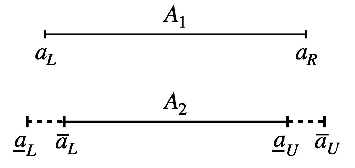
Definition 2.

The Type-2 interval is denoted by$A=\left[\left({\underset{\_}{a}}_L,{\overline{a}}_L\right),\left({\underset{\_}{a}}_U,{\overline{a}}_U\right)\right]$and defined in the form of Type-1 intervals given as

$$\left[\left({\underset{\_}{a}}_L,{\overline{a}}_L\right),\left({\underset{\_}{a}}_U,{\overline{a}}_U\right)\right]=\left\{\left[a_L,a_U\right]\hspace{0.17em}:a_L\in \left[{\underset{\_}{a}}_L,{\overline{a}}_L\right]\hspace{0.17em}\hspace{0.17em}\mathrm{and} a_U\in \left[{\underset{\_}{a}}_U,{\overline{a}}_U\right]\right\}.$$

Comparison of Type-1 and Type-2 interval:

Let $A=\left[\left({\underset{\_}{a}}_L,{\overline{a}}_L\right),\left({\underset{\_}{a}}_U,{\overline{a}}_U\right)\right]$ be a Type-2 interval. From the definition of the Type-2 interval, any element of $A_2$ is of the form Type-1 interval $A_1=\left[a_L,a_U\right],\hspace{0.17em}\hspace{0.17em}{a}_L\in \left[{\underset{\_}{a}}_L,{\overline{a}}_L\right]\hspace{0.17em}\&\hspace{0.17em}{a}_U\in \left[{\underset{\_}{a}}_U,{\overline{a}}_U\right]$. Thus, a Type-1 interval is a member of a Type-2 interval. From the definition, it is observed that the elements (Type-1 intervals) of $A_2$ with the largest and smallest widths are $\left[{\underset{\_}{a}}_L,{\overline{a}}_U\right]\hspace{0.17em}\hspace{0.17em}\mathrm{and} \left[{\overline{a}}_L,{\underset{\_}{a}}_U\right]$, respectively.

For example, let $A_2=\left[\left(-2,3\right),\left(6,8\right)\right]\hspace{0.17em}$. Then, the largest element of $A_2$ is $\left[-2,8\right]$ and the smallest one is $\left[3,6\right].$ Another intermediate element is $\left[1,7\right]\in A_2.$

A generic Type-2 interval $A_2=\left[\left({\underset{\_}{a}}_L,{\overline{a}}_L\right),\left({\underset{\_}{a}}_U,{\overline{a}}_U\right)\right]$ and a Type-1 interval $A_1=\left[a_L,a_U\right]\in A_2$ are shown graphically in Figure 1.

Definition 3.

Suppose$A=\left[\left({\underset{\_}{a}}_L,{\overline{a}}_L\right),\left({\underset{\_}{a}}_U,{\overline{a}}_U\right)\right]\hspace{0.17em}\hspace{0.17em},\hspace{0.17em}\hspace{0.17em}B=\left[\left({\underset{\_}{b}}_L,{\overline{b}}_L\right),\left({\underset{\_}{b}}_U,{\overline{b}}_U\right)\right]$are two Type-2 intervals. Now,$A=B$iff${\underset{\_}{a}}_L={\underset{\_}{b}}_L,{\overline{a}}_L={\overline{b}}_L,{\underset{\_}{a}}_U={\underset{\_}{b}}_U,{\overline{a}}_U={\overline{b}}_U.$

Definition 4.

Let$A=\left[\left({\underset{\_}{a}}_L,{\overline{a}}_L\right),\left({\underset{\_}{a}}_U,{\overline{a}}_U\right)\right]\hspace{0.17em}\hspace{0.17em},\hspace{0.17em}\hspace{0.17em}B=\left[\left({\underset{\_}{b}}_L,{\overline{b}}_L\right),\left({\underset{\_}{b}}_U,{\overline{b}}_U\right)\right]$be two Type-2 intervals. Then, the fundamental arithmetic operations between A and B are defined as follows:

(i) 

Addition:

$$A+B=\left[\left({\underset{\_}{a}}_L,{\overline{a}}_L\right),\left({\underset{\_}{a}}_U,{\overline{a}}_U\right)\right]+\left[\left({\underset{\_}{b}}_L,{\overline{b}}_L\right),\left({\underset{\_}{b}}_U,{\overline{b}}_U\right)\right]=\left[\left({\underset{\_}{a}}_L+{\underset{\_}{b}}_L,{\overline{a}}_L+{\overline{b}}_L\right),\left({\underset{\_}{a}}_U+{\underset{\_}{b}}_U,{\overline{a}}_U+{\overline{b}}_U\right)\right]$$

(ii) 

Subtraction:

$$A-B=\left[\left({\underset{\_}{a}}_L,{\overline{a}}_L\right),\left({\underset{\_}{a}}_U,{\overline{a}}_U\right)\right]-\left[\left({\underset{\_}{b}}_L,{\overline{b}}_L\right),\left({\underset{\_}{b}}_U,{\overline{b}}_U\right)\right]=\left[\left({\underset{\_}{a}}_L-{\overline{b}}_U,{\overline{a}}_L-{\underset{\_}{b}}_U\right),\left({\underset{\_}{a}}_U-{\overline{b}}_L,{\overline{a}}_U-{\underset{\_}{b}}_L\right)\right]$$

(iii) 

Scalar multiplication:

$$\lambda .A=\lambda .\left[\left({\underset{\_}{a}}_L,{\overline{a}}_L\right),\left({\underset{\_}{a}}_U,{\overline{a}}_U\right)\right]=\{\begin{array}{c}\left[\left(\lambda {\underset{\_}{a}}_L,\lambda {\overline{a}}_L\right),\left(\lambda {\underset{\_}{a}}_U,\lambda {\overline{a}}_U\right)\right]\hspace{0.17em}\hspace{0.17em}\mathrm{if} \lambda \ge 0,\\ \left[\left(\lambda {\overline{a}}_U,\lambda {\underset{\_}{a}}_U\right),\left(\lambda {\overline{a}}_L,\lambda {\underset{\_}{a}}_L\right)\right]\hspace{0.17em}\hspace{0.17em}\mathrm{if} \lambda <0.\end{array}$$

(iv) 

Multiplication:

$$\begin{array}{l}AB=\left[(\min C,\min D),(\max D,\max C)\right]\\ where\hspace{0.17em}\hspace{0.17em}C=\left\{{\underset{\_}{a}}_L{\underset{\_}{b}}_L,{\underset{\_}{a}}_L{\overline{b}}_U,{\overline{a}}_U{\overline{b}}_U,{\overline{a}}_U{\underset{\_}{b}}_L\right\},\hspace{0.17em}D=\left\{{\overline{a}}_L{\overline{b}}_L,{\underset{\_}{a}}_U{\overline{b}}_L,{\underset{\_}{a}}_U{\underset{\_}{b}}_U,{\underset{\_}{a}}_U{\overline{b}}_L\right\}\end{array}$$

(v) 

Division:

$$\frac{A}{B}=A.\left(\frac{1}{B}\right)\hspace{0.17em}\hspace{0.17em}provided 0\notin \mathrm{B}.$$

3. Type-2 Interval Order Relation

In this section, the order relation of two Type-2 intervals is defined and, to justify its validity, two numerical examples are considered.

Definition 5.

Let$A=\left[\left({\underset{\_}{a}}_L,{\overline{a}}_L\right),\left({\underset{\_}{a}}_U,{\overline{a}}_U\right)\right]$be a Type-2 interval. Then, a set of score functions of A which uniquely determines A is defined as$\left\{A_a^c,A_a^r,A_U^c,A_U^r\right\}$,

where

$$A_a^c=\frac{{\underset{\_}{a}}_L+{\overline{a}}_L+{\underset{\_}{a}}_U+{\overline{a}}_U}{4},\hspace{0.17em}{A}_a^r=\frac{{\overline{a}}_U-{\underset{\_}{a}}_U+{\overline{a}}_L-{\underset{\_}{a}}_L}{4},\hspace{0.17em}{A}_U^c=\frac{{\underset{\_}{a}}_U+{\overline{a}}_U}{2},A_U^r=\frac{{\overline{a}}_U-{\underset{\_}{a}}_U}{2}$$

Definition 6.

Let$A=\left[\left({\underset{\_}{a}}_L,{\overline{a}}_L\right),\left({\underset{\_}{a}}_U,{\overline{a}}_U\right)\right]\hspace{0.17em},\hspace{0.17em}B=\left[\left({\underset{\_}{b}}_L,{\overline{b}}_L\right),\left({\underset{\_}{b}}_U,{\overline{b}}_U\right)\right]$be two Type-2 intervals with corresponding sets of score functions$\left\{A_a^c,A_a^r,A_U^c,A_U^r\right\}\hspace{0.17em}\&\left\{B_a^c,B_a^r,B_U^c,B_U^r\right\}$, respectively.

Then

$$A{\le }_2^{}B\hspace{0.17em}iff\{\begin{array}{l}{A}_a^c\le B_a^c,\hspace{0.17em}\mathrm{if} A_a^c\ne B_a^c\\ A_a^r\le B_a^r,\hspace{0.17em}\mathrm{if} A_a^c=B_a^c\hspace{0.17em}\mathrm{and} A_a^r\ne B_a^r\\ A_U^c\le B_U^c,\hspace{0.17em}\mathrm{if} A_a^c=B_a^c\hspace{0.17em}, A_a^r=B_a^r \mathrm{and} A_U^c\ne B_U^c\\ A_U^r\le B_U^r,\hspace{0.17em}\mathrm{if} A_a^c=B_a^c\hspace{0.17em}, A_a^r=B_a^r \mathrm{and} A_U^c=B_U^c\end{array}$$

Definition 7.

Let$A=\left[\left({\underset{\_}{a}}_L,{\overline{a}}_L\right),\left({\underset{\_}{a}}_U,{\overline{a}}_U\right)\right]\hspace{0.17em},\hspace{0.17em}B=\left[\left({\underset{\_}{b}}_L,{\overline{b}}_L\right),\left({\underset{\_}{b}}_U,{\overline{b}}_U\right)\right]$be two Type-2 intervals. Then$A{\ge }_2^{}B\hspace{0.17em}\mathrm{iff}\hspace{0.17em}B{\le }_2^{}A.$

Example 1.

Compare the following pairs of Type-2 intervals by using Definition 6.

(i)

$$A=\left[\left(-4,-1\right),\left(2,5\right)\right]\hspace{0.17em},\hspace{0.17em}B=\left[\left(-6,-3\right),\left(-1,3\right)\right].$$

(ii)

$$A=\left[\left(-2,1\right),\left(4,7\right)\right]\hspace{0.17em},B=\left[\left(1,2\right),\left(3,4\right)\right]$$

Solution:

(i)

Here, $\left\{A_a^c,A_a^r,A_U^c,A_U^r\right\}=\left\{\frac{1}{2},\frac{3}{2},\frac{7}{2},\frac{3}{2}\right\}\hspace{0.17em}\&\left\{B_a^c,B_a^r,B_U^c,B_U^r\right\}=\left\{\frac{-7}{4},\frac{7}{4},1,2\right\}$.

Since $A_a^c=\frac{1}{2}>\frac{-7}{4}=B_a^c$, using Definition 6, we can say that $A{\ge }_2^{}B$.

(ii)

Here, $\left\{A_a^c,A_a^r,A_U^c,A_U^r\right\}=\left\{\frac{10}{4},\frac{3}{2},\frac{11}{2},\frac{3}{2}\right\}\hspace{0.17em}\&\left\{B_a^c,B_a^r,B_U^c,B_U^r\right\}=\left\{\frac{10}{4},\frac{1}{2},\frac{7}{2},\frac{1}{2}\right\}$.

Since $A_a^c=\frac{10}{4}=B_a^c\hspace{0.17em}\&A_a^r=\frac{3}{2}>\frac{1}{2}=B_a^r$ and using Definition 6, we can say that $A{\ge }_2^{}B$.

4. Optimality of Unconstrained Type-2 Interval-Valued Optimization Problem

Let $T\subseteq {\mathbb{R}}^n$ and $F_2:T\to I_2\left(\mathbb{R}\right)$ be a Type-2 interval-valued function given by $F_2\left(x\right)=\left[\left({\underset{\_}{f}}_L\left(x\right),{\overline{f}}_L\left(x\right)\right),\left({\underset{\_}{f}}_U\left(x\right),{\overline{f}}_U\left(x\right)\right)\right],\hspace{0.17em}{\underset{\_}{f}}_L,{\overline{f}}_L,{\underset{\_}{f}}_U,{\overline{f}}_U:T\to \mathbb{R}.$ Now the set of score functions of $F_2\left(x\right)$ is defined as $\left\{F_a^c,F_a^r,F_U^c,F_U^r\right\}$, where

$$\begin{array}{l}{F}_a^c\left(x\right)=\frac{{\underset{\_}{f}}_L\left(x\right)+{\overline{f}}_L\left(x\right)+{\underset{\_}{f}}_U\left(x\right)+{\overline{f}}_U\left(x\right)}{4},\hspace{0.17em}\\ F_a^r\left(x\right)=\frac{{\overline{f}}_L\left(x\right)-{\underset{\_}{f}}_L\left(x\right)+{\overline{f}}_U\left(x\right)-{\underset{\_}{f}}_U\left(x\right)}{4},\\ F_U^c\left(x\right)=\frac{{\underset{\_}{f}}_U\left(x\right)+{\overline{f}}_U\left(x\right)}{2}\hspace{0.17em}\hspace{0.17em}\mathrm{and} \hspace{0.17em}{F}_U^r\left(x\right)=\frac{{\overline{f}}_U\left(x\right)-{\underset{\_}{f}}_U\left(x\right)}{2}\end{array}$$

Definition 8.

The point$x^{\ast }\hspace{0.17em}\in T$is called a local minimizer of the Type-2 interval-valued function$F_2\left(x\right)$if$\exists \hspace{0.17em}\mathrm{a}\hspace{0.17em}\delta >0\hspace{0.17em}\mathit{such} \mathit{that}$$F_2\left(x^{*}\right){\le }_2^{}{F}_2\left(x\right),\hspace{0.17em}\forall x\in N\left(x^{\ast },\delta \right)\cap T,$where$N(x^{*},\delta )$is an open ball centered at$x^{*}$with radius$\delta$and${\le }_2^{}$is the symbol of Type-2 interval order relation as defined in Definition 6.

Definition 9.

The point$x^{\ast }\hspace{0.17em}\in T$is called a global minimizer of$F_2\left(x\right)$if$\exists \hspace{0.17em}\mathrm{a}\hspace{0.17em}\delta >0\hspace{0.17em}\mathit{such} \mathit{that}$$F_2\left(x^{*}\right){\le }_2^{}{F}_2\left(x\right),\hspace{0.17em}\forall x\in T$.

Definition 10.

The point$x^{\ast }\hspace{0.17em}\in T$is called a local maximizer of$F_2\left(x\right)$if$\exists \hspace{0.17em}\mathrm{a}\hspace{0.17em}\delta >0\hspace{0.17em}such that F_2\left(x^{*}\right){\ge }_2^{}{F}_2\left(x\right),\hspace{0.17em}\forall x\in N\left(x^{\ast },\delta \right)\cap T.$

Definition 11.

The point$x^{\ast }\hspace{0.17em}\in T$is called a global maximizer of$F_2\left(x\right)$if$\exists \hspace{0.17em}\mathrm{a}\hspace{0.17em}\delta >0\hspace{0.17em}such that F_2\left(x^{*}\right){\ge }_2^{}{F}_2\left(x\right),\hspace{0.17em}\forall x\in T.$

Theorem 1 (Necessary Optimality Conditions).

Let$T\subseteq {\mathbb{R}}^n$and$F_2:T\to I_2\left(\mathbb{R}\right)$be a Type-2 interval-valued function defined by$F_2\left(x\right)=\left[\left({\underset{\_}{f}}_L\left(x\right),{\overline{f}}_L\left(x\right)\right),\left({\underset{\_}{f}}_U\left(x\right),{\overline{f}}_U\left(x\right)\right)\right]$and all the elements of the set of score functions$\left\{F_a^c,F_a^r,F_U^c,F_U^r\right\}$are supposed to be differentiable, i.e.,$\nabla F_a^c,\nabla F_a^r,\nabla F_U^c \mathrm{and} \nabla F_U^r$exist.

$$\begin{array}{l}{F}_a^c\left(x\right)=\frac{{\underset{\_}{f}}_L\left(x\right)+{\overline{f}}_L\left(x\right)+{\underset{\_}{f}}_U\left(x\right)+{\overline{f}}_U\left(x\right)}{4},\hspace{0.17em}\\ F_a^r\left(x\right)=\frac{{\overline{f}}_L\left(x\right)-{\underset{\_}{f}}_L\left(x\right)+{\overline{f}}_U\left(x\right)-{\underset{\_}{f}}_U\left(x\right)}{4},\\ F_U^c\left(x\right)=\frac{{\underset{\_}{f}}_U\left(x\right)+{\overline{f}}_U\left(x\right)}{2}\hspace{0.17em}\hspace{0.17em}and \hspace{0.17em}{F}_U^r\left(x\right)=\frac{{\overline{f}}_U\left(x\right)-{\underset{\_}{f}}_U\left(x\right)}{2}\end{array}$$

Then,$x^{\ast }\hspace{0.17em}\in T$be an optimizer of Type-2 interval-valued function$F_2\left(x\right)$, if

$$\begin{array}{l}\nabla F_a^c\left(x^{\ast }\right)=0 \mathit{when} F_a^c\left(x\right)\hspace{0.17em}\ne \mathit{constant}\\ \nabla F_a^r\left(x^{\ast }\right)=0 \mathit{when} F_a^c\left(x\right)\hspace{0.17em}=\mathit{constant} \mathit{and} F_a^r\left(x\right)\ne \mathit{constant} \\ \nabla F_U^c\left(x^{*}\right)=0\hspace{0.17em}\mathit{when} \mathit{both} F_a^c\left(x\right)\hspace{0.17em}\mathit{and} F_a^r\left(x\right)\mathit{are} \mathit{constant} \mathit{and} F_U^c\left(x\right)\ne \mathit{constant}\\ \nabla F_U^r\left(x^{*}\right)=0\hspace{0.17em}\mathit{when} \mathit{all} \hspace{0.17em}{F}_a^c\left(x\right)\hspace{0.17em},F_a^r\left(x\right) \mathit{and} F_U^c\left(x\right) \mathit{are} \mathit{constant}\end{array}$$

Proof. 

Here, Theorem 1 is proved only for the minimization case. The maximization case can be proved similarly. Suppose $x^{\ast }\hspace{0.17em}\in T$ is a local minimizer of $F_2\left(x\right)$. Now, the definition of local minimizer implies that $F_2\left(x^{\ast }\right){\le }_2^{}{F}_2\left(x\right)\hspace{0.17em}\forall x\in T\cap N\left(x^{\ast },\delta \right)$,

i.e.,

$$\begin{array}{l}{F}_a^c\left(x^{\ast }\right)\le F_a^c\left(x\right) \mathrm{when}{F}_a^c\left(x^{*}\right)\hspace{0.17em} \ne F_a^c\left(x\right)\\ F_a^r\left(x^{\ast }\right)\le F_a^r\left(x\right) \mathrm{when} F_a^c\left(x^{*}\right)\hspace{0.17em}=F_a^c\left(x\right) \mathrm{and} F_a^r\left(x^{*}\right)\ne F_a^r\left(x\right)\\ F_U^c\left(x^{*}\right)\hspace{0.17em}\le F_U^c\left(x\right)\mathrm{when} F_a^c\left(x^{*}\right)=F_a^c\left(x\right)\hspace{0.17em}, F_a^r\left(x^{*}\right)=F_a^r\left(x\right)\mathrm{and} F_U^c\left(x^{*}\right)\ne F_U^c\left(x\right)\\ F_U^r\left(x^{*}\right)\le F_U^r\left(x\right) \mathrm{when} F_a^c\left(x^{*}\right)=F_a^c\left(x\right)\hspace{0.17em}, F_a^r\left(x^{*}\right)=F_a^r\left(x\right)\mathrm{and} F_U^c\left(x^{*}\right)=F_U^c\left(x\right)\end{array}$$

The earlier mentioned relations mean that

$$\begin{array}{l}{F}_a^c\left(x^{\ast }\right)\le F_a^c\left(x\right) \mathrm{when}{F}_a^c\left(x\right)\mathrm{is} \mathrm{non} \mathrm{constant}\\ F_a^r\left(x^{\ast }\right)\le F_a^r\left(x\right) \mathrm{when} F_a^c\left(x\right)\hspace{0.17em}\mathrm{is} \mathrm{constant} \mathrm{and} F_a^r\left(x\right) \mathrm{is} \mathrm{non} \mathrm{constant}\\ F_U^c\left(x^{*}\right)\hspace{0.17em}\le F_U^c\left(x\right)\mathrm{when} F_a^c\left(x\right)\hspace{0.17em}, F_a^r\left(x\right)\mathrm{are} \mathrm{constant} \mathrm{and} F_U^c\left(x\right)\mathrm{is} \mathrm{non}-\mathrm{constant}\\ F_U^r\left(x^{*}\right)\le F_U^r\left(x\right) \mathrm{when} \mathrm{all} F_a^c\left(x\right)\hspace{0.17em},F_a^r\left(x\right)\mathrm{and} F_U^c\left(x\right)\mathrm{are} \mathrm{constants}\end{array}$$

Thus, $x^{\ast }\hspace{0.17em}\in T$ is a local minimizer for

$$\begin{array}{l}{F}_c^c\left(x\right) \mathrm{when}{F}_a^c\left(x\right)\mathrm{is} \mathrm{non} \mathrm{constant}\\ F_U^c\left(x\right) \mathrm{when} F_a^c\left(x\right)\hspace{0.17em}\mathrm{is} \mathrm{constant} \mathrm{and} F_a^r\left(x\right) \mathrm{is} \mathrm{non} \mathrm{constant}\\ F_U^r\left(x\right) \mathrm{when} F_a^c\left(x\right)\hspace{0.17em}, F_a^r\left(x\right)\mathrm{are} \mathrm{constant} \mathrm{and} F_U^c\left(x\right)\mathrm{is} \mathrm{non}-\mathrm{constant}\\ F_c^r\left(x\right)\mathrm{when} \mathrm{all} F_a^c\left(x\right)\hspace{0.17em},F_a^r\left(x\right)\mathrm{and} F_U^c\left(x\right)\mathrm{are} \mathrm{constants}\end{array}$$

Then, according to the necessary optimality conditions for crisp minimization problem with real-valued objectives, $F_a^c\left(x\right),F_a^r\left(x\right),F_U^c\left(x\right)\hspace{0.17em}\mathrm{and} F_U^r\left(x\right),$ we get

$$\begin{array}{l}\nabla F_a^c\left(x^{\ast }\right)=0 \mathrm{when} F_a^c\left(x\right)\hspace{0.17em}\ne \mathrm{constant}\\ \nabla F_a^r\left(x^{\ast }\right)=0 \mathrm{when} F_a^c\left(x\right)\hspace{0.17em}=\mathrm{constant} \mathrm{and} F_a^r\left(x\right)\ne \mathrm{constant} \\ \nabla F_U^c\left(x^{*}\right)=0\hspace{0.17em}\mathrm{when} \mathrm{both} F_a^c\left(x\right)\hspace{0.17em}\mathrm{and} F_a^r\left(x\right)\mathrm{are} \mathrm{constant} \mathrm{and} F_U^c\left(x\right)\ne \mathrm{constant}\\ \nabla F_U^r\left(x^{*}\right)=0\hspace{0.17em}\mathrm{when} \mathrm{all} \hspace{0.17em}{F}_a^c\left(x\right)\hspace{0.17em},F_a^r\left(x\right) \mathrm{and} F_U^c\left(x\right) \mathrm{are} \mathrm{constant}\end{array}$$

                        □

Definition 12.

Let$f:T\subseteq {\mathbb{R}}^n\to \mathbb{R}$be a twice differentiable crisp function. Then, the Hessian matrix${\nabla }^{2}f\left(x\right) \mathrm{of} f$is defined by the$n\times n$matrix whose entries are the second-order partial derivatives, i.e.,${\nabla }^{2}f\left(x\right)={\left(\frac{{\partial }^{2}f}{\partial x_i\partial x_j}\right)}_{n\times n}.$

Theorem 2 (Sufficient Conditions).

Let$F_2:T\to I_2\left(\mathbb{R}\right)$be given in the form$F_2\left(x\right)=\left[\left({\underset{\_}{f}}_L\left(x\right),{\overline{f}}_L\left(x\right)\right),\left({\underset{\_}{f}}_U\left(x\right),{\overline{f}}_U\left(x\right)\right)\right]$.

Suppose$x^{\ast }\hspace{0.17em}\in T$is such that each element of the set of score functions$\left\{F_a^c,F_a^r,F_U^c,F_U^r\right\}$of$F_2$is differentiable and satisfies the following conditions:

$$\begin{array}{l}\nabla F_a^c\left(x^{\ast }\right)=0 \mathit{when} F_a^c\left(x\right)\hspace{0.17em}\ne \mathit{constant}\\ \nabla F_a^r\left(x^{\ast }\right)=0 \mathit{when} F_a^c\left(x\right)\hspace{0.17em}=\mathit{constant} \mathit{and} F_a^r\left(x\right)\ne \mathit{constant} \\ \nabla F_U^c\left(x^{*}\right)=0\hspace{0.17em}\mathit{when} \mathit{both} F_a^c\left(x\right)\hspace{0.17em}\mathit{and} F_a^r\left(x\right)\mathit{are} \mathit{constant} \mathit{and} F_U^c\left(x\right)\ne \mathit{constant}\\ \nabla F_U^r\left(x^{*}\right)=0\hspace{0.17em}\mathit{when} \mathit{all} \hspace{0.17em}{F}_a^c\left(x\right)\hspace{0.17em},F_a^r\left(x\right) \mathit{and} F_U^c\left(x\right) \mathit{are} \mathit{constant}\end{array}$$

(i) Then,$x^{\ast }\hspace{0.17em}\in T$is a local minimizer of$F_2$if

$$\begin{array}{l}{\nabla }^2{F}_a^c\left(x^{\ast }\right)\mathit{be} \mathit{positive} \mathit{definite} \mathit{when} F_a^c\left(x\right)\hspace{0.17em}\ne \mathit{constant} \\ {\nabla }^2{F}_a^r\left(x^{\ast }\right) \mathit{be} \mathit{positive} \mathit{definite} \mathit{when} F_a^c\left(x\right)\hspace{0.17em}=\mathit{constant} \mathit{and} F_a^r\left(x\right)\ne \mathit{constant}\\ {\nabla }^2{F}_U^c\left(x^{*}\right)\mathit{be} \mathit{positive} \mathit{definite} \mathit{when} \mathit{both} F_a^c\left(x\right)\hspace{0.17em}\mathit{and} F_a^r\left(x\right)\mathit{are} \mathit{constant} \mathit{and} F_U^c\left(x\right)\ne \mathit{constant}\\ {\nabla }^2{F}_U^r\left(x^{*}\right) \mathit{be} \mathit{positive} \mathit{definite} \mathit{when} \mathit{all} \hspace{0.17em}{F}_a^c\left(x\right)\hspace{0.17em},F_a^r\left(x\right)\mathit{and} F_U^c\left(x\right) \mathit{are} \mathit{constant}\end{array}$$

(ii)$x^{\ast }\hspace{0.17em}\in T$is local maximizer of$F_2$if

$$\begin{array}{l}{\nabla }^2{F}_a^c\left(x^{\ast }\right)\mathit{be} \mathit{negetive} \mathit{definite} \mathit{when} F_a^c\left(x\right)\hspace{0.17em}\ne \mathit{constant} \\ {\nabla }^2{F}_a^r\left(x^{\ast }\right) \mathit{be} \mathit{negetive} \mathit{definite} \mathit{when} F_a^c\left(x\right)\hspace{0.17em}=\mathit{constant} \mathit{and} F_a^r\left(x\right)\ne \mathit{constant}\\ {\nabla }^2{F}_U^c\left(x^{*}\right)\mathit{be} \mathit{negetive} \mathit{definite} \mathit{when} \mathit{both} F_a^c\left(x\right)\hspace{0.17em}\mathit{and} F_a^r\left(x\right)\mathit{are} \mathit{constant} \mathit{and} F_U^c\left(x\right)\ne \mathit{constant}\\ {\nabla }^2{F}_U^r\left(x^{*}\right) \mathit{be} \mathit{negetive} \mathit{definite} \mathit{when} \mathit{all} \hspace{0.17em}{F}_a^c\left(x\right)\hspace{0.17em},F_a^r\left(x\right)\mathit{and} F_U^c\left(x\right) \mathit{are} \mathit{constant}\end{array}$$

Proof. 

(i) To prove Theorem 2 (i), four cases may arise:

Case-I: when $F_a^c\left(x\right)\hspace{0.17em} \ne \mathrm{constant}$ with $\nabla F_a^c\left(x^{\ast }\right)=0 \mathrm{and} {\nabla }^2{F}_a^c\left(x^{\ast }\right)$ is positive definite at $x^{\ast }\hspace{0.17em}\in T$. Then, from the sufficient optimality condition for real-valued function, $F_a^c$ we have

$$F_a^c(x^{\ast })\le F_a^c\left(x\right)\hspace{0.17em},\hspace{0.17em}\forall x\in T\cap N\left(x^{\ast },{\delta }_1\right)$$

where $N\left(x^{\ast },{\delta }_1\right)$ is an open ball whose center is at $x^{\ast }$ with radius ${\delta }_1.$

Case-II: when $F_a^c\left(x\right)\hspace{0.17em}=\mathrm{constant} \mathrm{and} F_a^r\left(x\right)\ne \mathrm{constant}$ with

$\nabla F_a^r\left(x^{\ast }\right)=0\hspace{0.17em}\mathrm{and} {\nabla }^2{F}_a^r\left(x^{\ast }\right)$ is positive definite at $x^{\ast }\hspace{0.17em}\in T$.

$$\mathrm{Then} F_a^r(x^{\ast })\le F_a^r\left(x\right)\hspace{0.17em},\hspace{0.17em}\forall x\in T\cap N\left(x^{\ast },{\delta }_2\right)$$

$$\mathrm{where} {\delta }_2\hspace{0.17em}\mathrm{is} \mathrm{the} \mathrm{radius} \mathrm{of} \mathrm{the} \mathrm{open} \mathrm{ball} N\left(x^{*},{\delta }_2\right)\mathrm{with} \mathrm{centre} \mathrm{at} x^{\ast }.$$

Similarly,

Case-III: when $F_a^c\left(x\right),F_a^r\left(x\right)=\mathrm{constant} \mathrm{and} F_U^c\left(x\right)\ne \mathrm{constant}$

with $\nabla F_U^c\left(x^{\ast }\right)=0\hspace{0.17em}\mathrm{and} {\nabla }^2{F}_U^c\left(x^{\ast }\right)$ is positive definite at $x^{\ast }\hspace{0.17em}\in T$.

$$\mathrm{Then} F_U^c(x^{\ast })\le F_U^c\left(x\right)\hspace{0.17em},\hspace{0.17em}\forall x\in T\cap N\left(x^{\ast },{\delta }_3\right)$$

$$\mathrm{where} {\delta }_3\hspace{0.17em}\mathrm{is} \mathrm{the} \mathrm{radius} \mathrm{of} \mathrm{open} \mathrm{ball} \mathrm{with} \mathrm{centre} \mathrm{at} x^{\ast }.$$

Case-IV:

when $F_a^c\left(x\right),F_a^r\left(x\right),\hspace{0.17em}{F}_U^c\left(x\right) \mathrm{are} \mathrm{constants} \mathrm{and} F_U^r\left(x\right)\ne \mathrm{constant}$ with

$\nabla F_U^r\left(x^{\ast }\right)=0\hspace{0.17em}\mathrm{and} {\nabla }^2{F}_U^r\left(x^{\ast }\right)$ is positive definite at $x^{\ast }\hspace{0.17em}\in T$.

Then

$$F_U^r(x^{\ast })\le F_U^r\left(x\right)\hspace{0.17em},\hspace{0.17em}\forall x\in T\cap N\left(x^{\ast },{\delta }_4\right)$$

$$\begin{gathered} \mathrm{where} {\delta }_4\hspace{0.17em}\mathrm{is} \mathrm{the} \mathrm{radius} \mathrm{of} \mathrm{open} \mathrm{ball} \mathrm{with} \mathrm{centre} \mathrm{at} x^{\ast }. \\ \mathrm{Let} \mathrm{us} \mathrm{take} \end{gathered}$$

$$\delta =\min \left\{{\delta }_1,{\delta }_2,{\delta }_3,{\delta }_4\right\}.$$

Now, combining all the cases (I–IV), we get

$$\begin{array}{l}\hspace{0.17em}\forall x\in T\cap N\left(x^{\ast },\delta \right),\\ F_a^c\left(x^{*}\right)\le F_a^c\left(x\right) \mathrm{when} F_a^c\left(x\right)\hspace{0.17em}\ne \mathrm{constant}\\ F_a^r\left(x^{*}\right)\le F_a^r\left(x\right) \mathrm{when} F_a^c\left(x\right)\hspace{0.17em}=\mathrm{constant} \mathrm{and} F_a^r\left(x\right)\ne \mathrm{constant}\\ F_U^c\left(x^{*}\right)\le F_U^c\left(x\right) \mathrm{when} \mathrm{both} F_a^c\left(x\right)\hspace{0.17em}\mathrm{and} F_a^r\left(x\right)\mathrm{are} \mathrm{constant} \mathrm{and} F_U^c\left(x\right)\ne \mathrm{constant}\\ F_U^r\left(x^{*}\right)\le F_U^r\left(x\right)\hspace{0.17em}\hspace{0.17em} \mathrm{when} \mathrm{all} \hspace{0.17em}{F}_a^c\left(x\right)\hspace{0.17em},F_a^r\left(x\right)\mathrm{and} F_U^c\left(x\right) \mathrm{are} \mathrm{constant}\end{array}$$

So, by the definition of order relation, we get

$$F_2\left(x^{\ast }\right){\le }_2^{}{F}_2\left(x\right),\hspace{0.17em}\forall x\in T\cap N\left(x^{\ast },\delta \right).$$

Therefore, $x^{\ast }\hspace{0.17em}\in T$ is the local minimizer of $F_2$.

(ii) Similarly, the proof of the maximization case can be obtained.

□

Example 2.

Let us consider the following function for optimization.

$$F_2\left(x_1,x_2\right)=\left[\left(-6\left(x_1^2+x_2^2\right)-2,\left(x_1^2+x_2^2\right)\right),\left(\left(x_1^2+x_2^2\right)+3,6\left(x_1^2+x_2^2\right)+6\right)\right].\hspace{0.17em}$$

(1)

Solution:

Here we have:

$$\hspace{0.17em}{F}_a^c\left(x_1,x_2\right)=\frac{7}{2}=\mathrm{constant}.\hspace{0.17em}\mathrm{and}\hspace{0.17em}{F}_a^r\left(x_1,x_2\right)=3\left(x_1^2+x_2^2\right)+\frac{5}{4}$$

Therefore, for maximization or minimization of $F_2$, it is sufficient to minimize $F_a^r.$ Clearly, (0, 0) is the minimizer of $F_a^r$, and hence it is the minimizer of $F_2\left(x_1,x_2\right)$. Therefore, the minimum value of $F_2\left(x_1,x_2\right)$ at $\left(0,0\right)$ is $F_2\left(0,0\right)=\left[\left(-2,0\right), \left(3,6\right)\right]$.

Example 3.

Let us consider the following function for optimization:

$$F_2\left(x_1,x_2\right)=\left[\left(-3x_1^2{x}_2^2-1,-x_1^2{x}_2^2\right),\left(2\left(x_1^2+x_2^2\right)+1,2\left(x_1^2+x_2^2\right)+4\right)\right]\hspace{0.17em}\hspace{0.17em}\hspace{0.17em}\hspace{0.17em}\hspace{0.17em}\hspace{0.17em}\hspace{0.17em}\hspace{0.17em}\hspace{0.17em}$$

(2)

Solution: Here

$$F_a^c\left(x_1,x_2\right)=x_1^2+x_2^2-x_1^2{x}_2^2+1\ne \mathrm{constant}.$$

Therefore, the necessary conditions for optimality of $F_a^c\left(x_1,x_2\right)$ are given by

$$\frac{\partial F_a^c\left(x_1,x_2\right)}{\partial x_1}=2x_1-2x_1{x}_2^2=0\hspace{0.17em}$$

(3)

$$\hspace{0.17em}\frac{\partial F_a^c\left(x_1,x_2\right)}{\partial x_2}=2x_2-2x_1^2{x}_2=0\hspace{0.17em}\hspace{0.17em}$$

(4)

which implies

$$x_1=0,\pm 1\hspace{0.17em};\hspace{0.17em}{x}_2=0,\pm 1.$$

Hence the critical points of $F_a^c\left(x_1,x_2\right)$ are $\left(0,0\right),\left(1,1\right),\hspace{0.17em}\left(1,-1\right),\hspace{0.17em}\left(-1,1\right)\hspace{0.17em}\mathrm{and}\hspace{0.17em}\left(-1,-1\right).$

Now,

$${\nabla }^2{F}_a^c\left(x_1,x_2\right)=\left(\begin{array}{cc}2-2x_2^2& -4x_1{x}_2\\ -4x_1{x}_2& 2-2x_2^2\end{array}\right)$$

Clearly, ${\nabla }^2{F}_a^c\left(0,0\right)$ is the positive definite matrix. Thus,$\left(0,0\right)$ is the local minimizer of $F_2\left(x_1,x_2\right)$ and the minimum value of $F_2\left(x_1,x_2\right)$ is $F_2\left(0,0\right)=\left[\left(-1,0\right),\left(1,4\right)\right].$

At $\left(\pm 1,\pm 1\right)$, no definite conclusion has been made because, at these points, the strict definiteness of the Hessian matrix cannot be decided.

Definition 13.

Let$F_2\left(x\right)$be a Type-2 interval-valued function defined on$X\subseteq {\mathbb{R}}^n$with X being convex. Then,$F_2\left(x\right)$is said to be convex on X if$F_2\left(\lambda x_1+\left(1-\lambda \right)x_2\right){\le }_2^{}\lambda F_2\left(x_1\right)+\left(1-\lambda \right)F_2\left(x_2\right)$for each$\lambda \in \left(0,1\right)\hspace{0.17em}and \forall x_1,x_2\in X.$

Proposition 1.

Let$X\subseteq {\mathbb{R}}^n$be convex and$F_2$be a Type-2 interval-valued function given by$F_2\left(x\right)=\left[\left({\underset{\_}{f}}_L\left(x\right),{\overline{f}}_L\left(x\right)\right),\left({\underset{\_}{f}}_U\left(x\right),{\overline{f}}_U\left(x\right)\right)\right]$. If$F_a^c\left(x\right),F_a^r\left(x\right),F_U^c\left(x\right)\hspace{0.17em}and F_U^r\left(x\right)$are convex, then$F_2\left(x\right)$is convex.

5. Optimality Conditions of Constrained Type-2 Interval-Valued Optimization Problem

Let the general form of a nonlinearly constrained Type-2 interval-valued optimization problem be of the form:

$$\begin{array}{l}(MP)\hspace{0.17em}\hspace{0.17em}Minimize\hspace{0.17em}{F}_2\left(x\right)=\left[\left({\underset{\_}{f}}_L\left(x\right),{\overline{f}}_L\left(x\right)\right),\left({\underset{\_}{f}}_U\left(x\right),{\overline{f}}_U\left(x\right)\right)\right]\\ \mathrm{subject} \mathrm{to} G_i\left(x\right)\le \hspace{0.17em}or\hspace{0.17em}{\le }^{\min }\hspace{0.17em}or\hspace{0.17em}{\le }_2^{}{B}_i,\hspace{0.17em}i=1,2,\dots ,m.\end{array}$$

where

$$F_2:S\subseteq {\mathbb{R}}^n\to I_2\left(\mathbb{R}\right),\hspace{0.17em}{G}_i:S\to \mathbb{R}\hspace{0.17em}\mathrm{or} I_1\left(\mathbb{R}\right)\hspace{0.17em}or\hspace{0.17em}{I}_2\left(\mathbb{R}\right)$$

The definition of the order relation $\hspace{0.17em}{\le }_2^{}$ is given in Definition 6.

The definition of interval order relation ${\le }^{\min }$ was proposed by Bhunia and Samanta [29], defined in Definition 1.

The set of score functions of $F_2\left(x\right)$ is $\left\{F_a^c,F_a^r,F_U^c,F_U^r\right\}$, where

$$\begin{array}{l}{F}_a^c\left(x\right)=\frac{{\underset{\_}{f}}_L\left(x\right)+{\overline{f}}_L\left(x\right)+{\underset{\_}{f}}_U\left(x\right)+{\overline{f}}_U\left(x\right)}{4},\hspace{0.17em}\hspace{0.17em}{F}_a^r\left(x\right)=\frac{{\overline{f}}_L\left(x\right)-{\underset{\_}{f}}_L\left(x\right)+{\overline{f}}_U\left(x\right)-{\underset{\_}{f}}_U\left(x\right)}{4},\\ F_U^c\left(x\right)=\frac{{\underset{\_}{f}}_U\left(x\right)+{\overline{f}}_U\left(x\right)}{2}\hspace{0.17em}\hspace{0.17em}\mathrm{and} F_U^r\left(x\right)=\frac{{\overline{f}}_U\left(x\right)-{\underset{\_}{f}}_U\left(x\right)}{2}\end{array}$$

and let

$$S=\left\{x\in {\mathbb{R}}^n:G_i\left(x\right)\le \hspace{0.17em}or\hspace{0.17em}{\le }^{\min }\hspace{0.17em}or\hspace{0.17em}{\le }_2^{}{B}_i,i=1,2,\dots ,m\right\}$$

Definition 14.

The point$x^{\ast }\in S$is called a minimizer of the problem$(MP)$ if $F_2\left(x^{\ast }\right){\le }_2^{}{F}_2\left(x\right)\hspace{0.17em}\forall x\in S\cap N\left(x^{\ast },\delta \right)\hspace{0.17em}$, where $N\left(x^{\ast },\delta \right)$ is an open ball centered at $x^{\ast }\hspace{0.17em}and radius \delta .$

Optimality conditions:

Now, based on the nature of all constraints, $G_i\left(x\right)$, three cases may arise:

Case-1: when $F_2\left(x\right)$ is a Type-2 interval-valued function and all $G_i\left(x\right)\hspace{0.17em}(i=1,2,3,\dots ,m)$ are crisp functions (real-valued) having continuous partial derivatives up to the second order. In this case, the nonlinear Type-2 interval-valued constrained optimization problem along with inequality constraints can be expressed as follows:

$$\begin{array}{l}(MP1)\hspace{0.17em}\hspace{0.17em}Minimize\hspace{0.17em}{F}_2\left(x\right)=\left[\left({\underset{\_}{f}}_L\left(x\right),{\overline{f}}_L\left(x\right)\right),\left({\underset{\_}{f}}_U\left(x\right),{\overline{f}}_U\left(x\right)\right)\right]\\ \mathrm{subject} \mathrm{to} G_i\left(x\right)\le \hspace{0.17em}{B}_i,\hspace{0.17em}i=1,2,\dots ,m.\end{array}$$

Here each element of the set of score functions of $F_2\left(x\right)$ is continuously differentiable, i.e., $F_c^c,F_c^r,F_r^c,F_r^r\hspace{0.17em}\mathrm{and} G_i\hspace{0.17em}:{\mathbb{R}}^n\to \mathbb{R}$ are continuously differentiable functions.

Necessary conditions:

Theorem 3.

Suppose$x^{*}$is a local minimizer of the constrained optimization problem (MP1) in which all the basic Type-2 interval-valued constraint qualifications hold. Then, there exist multipliers${\lambda }_i,\hspace{0.17em}i=1,2,3,\dots ,m$subject to the following conditions:

$$\nabla F_a^c\left(x^{\ast }\right)+{\displaystyle \sum _{i=1}^m{\lambda }_i\nabla G_i\left(x^{\ast }\right)=0\hspace{0.17em}.}$$

(5)

$${\lambda }_i{G}_i\left(x^{\ast }\right)=0\hspace{0.17em},\hspace{0.17em}i=1,2,3,\dots ,m$$

(6)

$$G_i\left(x^{\ast }\right)\le 0\hspace{0.17em},\hspace{0.17em}\forall i=1,2,3,\dots ,m\hspace{0.17em}\hspace{0.17em}$$

(7)

$$\hspace{0.17em}{\lambda }_i\ge 0\hspace{0.17em},\hspace{0.17em}i=1,2,3,\dots ,m\hspace{0.17em}$$

(8)

Proof. 

First of all, we have introduced the non-negative slack variable $y_i^2$ in the given inequality constraints (MP1), and we get the equality constraints $H_i\left(x\right)=G_i\left(x\right)+y_i^2=0,\hspace{0.17em}i=1,2,3,\dots ,m$.

Now, the corresponding Lagrange function of (MP1) is as follows:

$$\begin{array}{l}{L}_2\left(x,{\lambda }_i,y_i\right)=\left[\left({\underset{\_}{l}}_L\left(x,{\lambda }_i,y_i\right),{\overline{l}}_L\left(x,{\lambda }_i,y_i\right)\right),\left({\underset{\_}{l}}_U\left(x,{\lambda }_i,y_i\right),{\overline{l}}_U\left(x,{\lambda }_i,y_i\right)\right)\right]\\ \hspace{1em}\hspace{1em}\hspace{1em}\hspace{1em} =F_2\left(x\right)+{\displaystyle \sum _{i=1}^m{\lambda }_i\left(G_i\left(x\right)+y_i^2\right)}\\ =\left[\begin{array}{l}\left({\underset{\_}{f}}_L\left(x\right)+{\displaystyle \sum _{i=1}^m{\lambda }_i\left(G_i\left(x\right)+y_i^2\right)},{\overline{f}}_L\left(x\right)+{\displaystyle \sum _{i=1}^m{\lambda }_i\left(G_i\left(x\right)+y_i^2\right)}\right),\\ \hspace{0.17em}\hspace{0.17em}\hspace{0.17em}\hspace{0.17em}\hspace{0.17em}\hspace{0.17em}\hspace{0.17em}\hspace{0.17em}\hspace{0.17em}\hspace{0.17em}\hspace{0.17em}\hspace{0.17em}\hspace{0.17em}\hspace{0.17em}\hspace{0.17em}\hspace{0.17em}\hspace{0.17em}\left({\underset{\_}{f}}_U\left(x\right)+{\displaystyle \sum _{i=1}^m{\lambda }_i\left(G_i\left(x\right)+y_i^2\right)},{\overline{f}}_U\left(x\right)+{\displaystyle \sum _{i=1}^m{\lambda }_i\left(G_i\left(x\right)+y_i^2\right)}\right)\end{array}\right]\end{array}$$

Here $L_a^c\left(x,{\lambda }_i,y_i\right)=F_a^c\left(x\right)+{\displaystyle \sum _{i=1}^m{\lambda }_i\left(G_i\left(x\right)+y_i^2\right)\ne \mathrm{const}.},\hspace{0.17em}\lambda ={\left({\lambda }_1,{\lambda }_2,\dots ,{\lambda }_m\right)}^T$ are the Lagrange multipliers. Now from the necessary conditions of the Type-2 interval-valued unconstrained optimization problem, we get

$$\nabla L_a^c\left(x,{\lambda }_i,y_i\right)=0\hspace{0.17em},\hspace{0.17em}\sin \mathrm{ce} L_a^c\left(x,{\lambda }_i,y_i\right)\hspace{0.17em}\ne \hspace{0.17em}\mathrm{constant}.$$

That is

$$\frac{\partial L_a^c}{\partial x_k}=\frac{\partial F_a^c}{\partial x_k}+{\displaystyle \sum _{i=1}^m{\lambda }_i\frac{\partial G_i}{\partial x_k}}=0,k=1,2,\dots ,n\hspace{0.17em}and\hspace{0.17em}x=\left(x_1,x_2,\dots ,x_n\right)\hspace{0.17em}\hspace{0.17em}$$

(9)

$$\frac{\partial L_a^c}{\partial y_i}=2{\lambda }_i{y}_i=0\hspace{0.17em},\hspace{0.17em}i=1,2,\dots ,m\hspace{0.17em}$$

(10)

$$\frac{\partial L_a^c}{\partial {\lambda }_i}=G_i\left(x\right)+y_i^2=0,i=1,2,\dots ,m$$

(11)

From Equation (9), we have

$$\begin{array}{l}\left(\frac{\partial F_a^c}{\partial x_1},\frac{\partial F_a^c}{\partial x_2},\dots ,\frac{\partial F_a^c}{\partial x_n}\right)+{\displaystyle \sum _{i=1}^m{\lambda }_i\left(\frac{\partial G_i}{\partial x_1},\frac{\partial G_i}{\partial x_2},\dots ,\frac{\partial G_i}{\partial x_n}\right)}=0\\ \mathrm{i}.\mathrm{e}., \nabla F_a^c\left(x\right)+{\displaystyle \sum _{i=1}^m{\lambda }_i\nabla G_i\left(x\right)}=0\end{array}$$

$G_i\left(x\right)+y_i^2=0\hspace{0.17em}\mathrm{implies}\hspace{0.17em}{G}_i\left(x\right)\le 0\hspace{0.17em}as\hspace{0.17em}{y}_i^2\hspace{0.17em}\mathrm{be} \mathrm{the}\hspace{0.17em}\mathrm{slack}\hspace{0.17em}\mathrm{variables},\hspace{0.17em}i=1,2,3,\dots ,m$

From Equation (11), we obtain

$$2{\lambda }_i{y}_i=0\hspace{0.17em}\Rightarrow \hspace{0.17em}\mathrm{either}{\lambda }_i=0\hspace{0.17em}or\hspace{0.17em}{y}_i=0$$

If $y_i=0$ and ${\lambda }_i>0$, then $\frac{\partial L_a^c}{\partial {\lambda }_i}=0$ gives $G_i\left(x\right)=0.$

This implies, either ${\lambda }_i=0\hspace{0.17em}or\hspace{0.17em}{G}_i\left(x\right)=0,\hspace{0.17em}\mathrm{i}.\mathrm{e}., {\lambda }_i{G}_i\left(x\right)=0\hspace{0.17em}\mathrm{and} {\lambda }_i\ge 0.\hspace{0.17em}i=1,2,3,\dots ,m$,

Hence, we have obtained the required necessary conditions.

□

Note 1.

These conditions are similar to the KKT conditions of the nonlinear crisp optimization problem derived by Karush [27], Kuhn and Tucker [28]. Thus, these conditions can be called generalized KKT conditions.

Sufficient condition:

Theorem 4.

Let$(x^{\ast },\hspace{0.17em}{\lambda }_1,{\lambda }_2,\dots ,{\lambda }_m)$satisfy the conditions (5)–(8), and all the elements of the set of score functions of$F_2\left(x\right)\hspace{0.17em}\mathrm{i}.\mathrm{e}., F_a^c,F_a^r,F_U^c,F_U^r\hspace{0.17em}\mathit{and} \mathit{all}\hspace{0.17em}{G}_i$are the differentiable and convex functions with$F_a^c$as non-constant function. Then$x^{\ast }$is the global minimizer of the problem (MP1).

Proof. 

Since $F_a^c,F_a^r,F_U^c,F_U^r\hspace{0.17em}\mathrm{and} G_i\hspace{0.17em}:{\mathbb{R}}^n\to \mathbb{R}$ being continuously differentiable convex functions with $F_a^c\left(x\right)\ne \mathrm{constant} \mathrm{and} (x^{\ast },\hspace{0.17em}{\lambda }_1,{\lambda }_2,\dots ,{\lambda }_m)$ satisfying the necessary conditions (5)–(8), then from the sufficient optimality conditions of the crisp function $F_a^c\left(x\right)$, it can be concluded that $x^{\ast }$ is a global minimizer of $F_a^c\left(x\right).$

That is, $F_a^c\left(x^{\ast }\right)<F_a^c\left(x\right)\hspace{0.17em},\hspace{0.17em}\mathrm{as}\hspace{0.17em}{F}_a^c\left(x\right)\ne \mathrm{constant}$.

This implies, $F_2\left(x^{\ast }\right){\le }_2^{}{F}_2\left(x\hspace{0.17em}\right)\hspace{0.17em},\hspace{0.17em}\forall x\in S\subseteq {\mathbb{R}}^n$.

Thus, $x^{\ast }$ is a global minimizer of $F_2\left(x\right)$.

Case-2: when all $\hspace{0.17em}{G}_i\left(x\right)\hspace{0.17em}(i=1,2,3,\dots ,m)$ are interval-valued weakly differentiable functions, then the problem (MP) can be rewritten as:

$$\begin{array}{l}(MP2)\hspace{0.17em}\hspace{0.17em}Minimize\hspace{0.17em}{F}_2\left(x\right)=\left[\left({\underset{\_}{f}}_L\left(x\right),{\overline{f}}_L\left(x\right)\right),\left({\underset{\_}{f}}_U\left(x\right),{\overline{f}}_U\left(x\right)\right)\right]\\ \mathrm{subject} \mathrm{to} G_i\left(x\right)=\left[{\underset{\_}{G}}_i\left(x\right),{\overline{G}}_i\left(x\right)\right]{\le }^{\min }\hspace{0.17em}\left[0,0\right],\hspace{0.17em}i=1,2,3,\dots ,m.\end{array}$$

Without loss of generality, it is assumed that the first $k$ constraints $G_i\left(x\right)$ have non-constant centers, $i=1,2,3,\dots ,k,\hspace{0.17em}k\le m,$ and the remaining $(m-k)$ components of $G_i\left(x\right)$ have constant centers, $i=k+1,\dots ,m.$

Then, by using Bhunia and Samanta’s [29] interval order relation, the constraints of the problem (MP2) can be rewritten as:

$$\begin{array}{l}{G}_i\left(x\right)=\left[{\underset{\_}{G}}_i\left(x\right),{\overline{G}}_i\left(x\right)\right]{\le }^{\min }\left[0,0\right],\\ \Rightarrow \hspace{0.17em}\hspace{0.17em}\hspace{0.17em}{G}_i^c\left(x\right)<0,\hspace{0.17em}\hspace{0.17em}i=1,2,\dots ,k,\hspace{0.17em}\hspace{0.17em}k\le m.\\ \hspace{0.17em}\hspace{0.17em}\hspace{0.17em}\hspace{0.17em}\mathrm{and}\hspace{0.17em}{G}_j^r\left(x\right)=0,\hspace{0.17em}j=k+1,k+2,k+3,\dots ,m.\end{array}$$

Here, $G_i^c\left(x\right)\hspace{0.17em}{\mathrm{and} \mathrm{G}}_i^r\left(x\right)$ are the center and the radius of $G_i\left(x\right)$, respectively. Thus, (MP2) can be rewritten as:

$$\begin{array}{c}\left(\mathrm{MP}3\right) \mathrm{Minimize} F_2\left(x\right)=\left[\left({\underset{\_}{f}}_L\left(x\right),{\overline{f}}_L\left(x\right)\right),\left({\underset{\_}{f}}_U\left(x\right),{\overline{f}}_U\left(x\right)\right)\right]\\ \mathrm{subject} \mathrm{to} \left(\mathrm{i}\right)\hspace{0.17em}{G}_i^c\left(x\right)\le 0,\hspace{0.17em}i=1,2,3,\dots ,k\hspace{0.17em},k\le m\\ (ii)\hspace{0.17em}{G}_i^r\left(x\right)=0,\hspace{0.17em}j=k+1,\dots ,m.\end{array}$$

Now, using Case-1, the KKT conditions of the problem (MP2), i.e., of the (MP3) are derived as follows:

$$\nabla F_a^c\left(x\right)+{\displaystyle \sum _{i=1}^k{\lambda }_i{G}_i^c\left(x\right)}+{\displaystyle \sum _{j=k+1}^m{\mu }_j{G}_j^r\left(x\right)}=0,\hspace{0.17em}k\le m.\hspace{0.17em}\hspace{0.17em}$$

(12)

$${\lambda }_i{G}_i\left(x\right)=0\hspace{0.17em},\hspace{0.17em}i=1,2,3,\dots ,k\hspace{0.17em}\hspace{0.17em}$$

(13)

$$G_j^r\left(x\right)=0,\hspace{0.17em}j=k+1,k+2,k+2,\dots ,m$$

(14)

$$G_i^c\left(x\right)\le 0,\hspace{0.17em}i=1,2,3,\dots k\hspace{0.17em}$$

(15)

$${\lambda }_i\ge 0,\hspace{0.17em}i=1,2,3,\dots ,k.\hspace{0.17em}$$

(16)

Case-3: let all $G_i\left(x\right)\hspace{0.17em}(i=1,2,3,\dots ,m)$ be Type-2 interval-valued and weakly continuously differentiable functions. In this case, the problem is reformulated in the following way:

$$\begin{array}{l}(MP4)\hspace{0.17em}\hspace{0.17em}Minimize\hspace{0.17em}{F}_2\left(x\right)=\left[\left({\underset{\_}{f}}_L\left(x\right),{\overline{f}}_L\left(x\right)\right),\left({\underset{\_}{f}}_U\left(x\right),{\overline{f}}_U\left(x\right)\right)\right]\\ \mathrm{subject} \mathrm{to} G_i\left(x\right)=\left[\left({\underset{\_}{g}}_{iL}\left(x\right),{\overline{g}}_{iL}\left(x\right)\right),\left({\underset{\_}{g}}_{iU}\left(x\right),{\overline{g}}_{iU}\left(x\right)\right)\right]{\le }_2^{}\left[\left(0,0\right),\left(0,0\right)\right],\hspace{0.17em}i=1,2,\dots ,m.\end{array}$$

Then, using the definition of Type-2 interval order relation, the problem (MP4) can be reformulated as:

$$\begin{array}{l}(MP5)\hspace{0.17em}\hspace{0.17em}Minimize\hspace{0.17em}{F}_2\left(x\right)=\left[\left({\underset{\_}{f}}_L\left(x\right),{\overline{f}}_L\left(x\right)\right),\left({\underset{\_}{f}}_U\left(x\right),{\overline{f}}_U\left(x\right)\right)\right]\\ \mathrm{subject} \mathrm{to} G_i{}_a^c\left(x\right)<0\hspace{0.17em},\hspace{0.17em}i=1,2,\dots ,m_1\\ \hspace{0.17em}\hspace{0.17em}\hspace{0.17em}\hspace{0.17em}\hspace{0.17em}\hspace{0.17em}\hspace{0.17em}\hspace{0.17em}\hspace{0.17em}\hspace{0.17em}\hspace{0.17em}\hspace{0.17em}\hspace{0.17em}\hspace{0.17em}{G}_j{}_a^r\left(x\right)=0,\hspace{0.17em}\hspace{0.17em}j=1,2,\dots ,m_2\\ \hspace{0.17em}\hspace{0.17em}\hspace{0.17em}\hspace{0.17em}\hspace{0.17em}\hspace{0.17em}\hspace{0.17em}\hspace{0.17em}\hspace{0.17em}\hspace{0.17em}\hspace{0.17em}\hspace{0.17em}\hspace{0.17em}\hspace{0.17em}{G}_k{}_U^c\left(x\right)<0,\hspace{0.17em}\hspace{0.17em}\hspace{0.17em}k=1,2,\dots ,m_3\\ \hspace{0.17em}\hspace{0.17em}\hspace{0.17em}\hspace{0.17em}\hspace{0.17em}\hspace{0.17em}\hspace{0.17em}\hspace{0.17em}\hspace{0.17em}\hspace{0.17em}\hspace{0.17em}\hspace{0.17em}\hspace{0.17em}\hspace{0.17em}{G}_l{}_U^r\left(x\right)=0,\hspace{0.17em}\hspace{0.17em}\hspace{0.17em}l=1,2,\dots ,m_4\hspace{0.17em}\hspace{0.17em}\hspace{0.17em}and\hspace{0.17em}\hspace{0.17em}{m}_1+m_2+m_3+m_4=m\end{array}$$

where $\left\{G_i{}_a^c,\hspace{0.17em}{G}_i{}_a^r,G_i{}_U^c,G_i{}_U^r\right\}$ are the set of score functions of $G_i$.

Now, using Case-1, the generalized conditions of (MP5) are derived as follows:

$$\nabla F_a^c\left(x\right)+{\displaystyle \sum _{i=1}^{m_1}{\lambda }_i^1{G}_i{}_a^c\left(x\right)}+{\displaystyle \sum _{j=1}^{m_2}{\lambda }_j^2{G}_j{}_a^r\left(x\right)}+{\displaystyle \sum _{k=1}^{m_3}{\lambda }_k^3{G}_j{}_U^c\left(x\right)}+{\displaystyle \sum _{l=1}^{m_4}{\lambda }_l^4{G}_l{}_U^r\left(x\right)}=0\hspace{0.17em}\hspace{0.17em}$$

(17)

$${\lambda }_i{G}_i{}_a^c\left(x\right)=0\hspace{0.17em},\hspace{0.17em}i=1,2,\dots ,m_1\hspace{0.17em}$$

(18)

$${\lambda }_j^3{G}_j{}_a^r\left(x\right)=0,\hspace{0.17em}j=1,2,\dots ,m_3$$

(19)

$$G_i{}_a^c\left(x\right)<0,\hspace{0.17em}i=1,2,\dots m_1\hspace{0.17em}$$

(20)

$$G_j{}_a^r=0\hspace{0.17em},\hspace{0.17em}j=1,2,\dots ,m_2\hspace{0.17em}$$

(21)

$$G_k{}_U^c<0,\hspace{0.17em}k=1,2,\dots ,m_3$$

(22)

$$G_l{}_U^r=0,\hspace{0.17em}l=1,2,\dots ,m_4\hspace{0.17em}$$

(23)

$${\lambda }_i^1,{\lambda }_k^3\ge 0,\hspace{0.17em}i=1,2,\dots m_1,\hspace{0.17em}k=1,2,\dots ,m_3$$

(24)

□

Example 4.

Let us consider the Type-2 interval-valued minimization problem:

$$\begin{array}{l}Minimize\hspace{0.17em}{F}_2\left(x\right)=\left[\left(x^2+x,x^2+x+1\right),\hspace{0.17em}\left(x^2+3,x^2+4\right)\right]\hspace{0.17em}\hspace{0.17em}\hspace{0.17em}\hspace{0.17em}\hspace{0.17em}\hspace{0.17em}\hspace{0.17em}\hspace{0.17em}\hspace{0.17em}\hspace{0.17em}\hspace{0.17em}\hspace{0.17em}\hspace{0.17em}\hspace{0.17em}\hspace{0.17em}\hspace{0.17em}\hspace{0.17em}\hspace{0.17em}\hspace{0.17em}\hspace{0.17em}\hspace{0.17em}\hspace{0.17em}\hspace{0.17em}\hspace{0.17em}\hspace{0.17em}\hspace{0.17em}\hspace{0.17em}\hspace{0.17em}\hspace{0.17em}\hspace{0.17em}\hspace{0.17em}\hspace{0.17em}\hspace{0.17em}\hspace{0.17em}\hspace{0.17em}\hspace{0.17em}\hspace{0.17em}\hspace{0.17em}\hspace{0.17em}\hspace{0.17em}\hspace{0.17em}\hspace{0.17em}\hspace{0.17em}\\ \hspace{0.17em}\hspace{0.17em}\hspace{0.17em}\hspace{0.17em}\hspace{0.17em}\hspace{0.17em}\hspace{0.17em}\hspace{0.17em}\hspace{0.17em}\hspace{0.17em}\hspace{0.17em}\hspace{0.17em}\hspace{0.17em}\hspace{0.17em}\hspace{0.17em}\hspace{0.17em}\hspace{0.17em}\hspace{0.17em}\hspace{0.17em}\hspace{0.17em}\hspace{0.17em}\hspace{0.17em}subject to x-2\le 0,\hspace{0.17em}-x\le 0\end{array}$$

(25)

Solution: Suppose $g_1\left(x\right)=x-2,\hspace{0.17em}{g}_2\left(x\right)=-x.$

Here, $F_a^c\left(x\right)=\frac{2x^2+x+4}{2}\ne \mathrm{constant}\hspace{0.17em}$.

Clearly, $F_a^c,\hspace{0.17em}{g}_1,\hspace{0.17em}{g}_2$ are continuously differentiable and convex functions. Then, the generalized KKT conditions of (25) are

$$2x^{\ast }+\frac{1}{2}+{\lambda }_1-{\lambda }_2=0\hspace{0.17em}\hspace{0.17em}\hspace{0.17em}$$

(26)

$${\lambda }_1\left(x^{\ast }-2\right)=-{\lambda }_2{x}^{\ast }=0$$

(27)

$$x^{\ast }-2\le 0,\hspace{0.17em}-x^{\ast }\le 0$$

(28)

$${\lambda }_1\ge 0,\hspace{0.17em}{\lambda }_2\ge 0$$

(29)

Clearly, $x^{\ast }=0,\hspace{0.17em}{\lambda }_1=0,\hspace{0.17em}{\lambda }_2=\frac{1}{2}$ satisfy the conditions (26)–(29). Therefore,$x^{\ast }=0$ is a global minimizer of (25).

Example 5.

Let us consider a minimization problem for Case-2 as follows:

$$\begin{array}{l}Minimize f\left(x\right)=\left[\left(x^2,x^2+2x\right),\left(x^2+4,x^2+2x+4\right)\right]\hspace{0.17em}\hspace{0.17em}\hspace{0.17em}\hspace{0.17em}\hspace{0.17em}\hspace{0.17em}\hspace{0.17em}\hspace{0.17em}\hspace{0.17em}\hspace{0.17em}\hspace{0.17em}\hspace{0.17em}\hspace{0.17em}\hspace{0.17em}\hspace{0.17em}\hspace{0.17em}\hspace{0.17em}\hspace{0.17em}\hspace{0.17em}\hspace{0.17em}\hspace{0.17em}\hspace{0.17em}\hspace{0.17em}\hspace{0.17em}\hspace{0.17em}\hspace{0.17em}\hspace{0.17em}\hspace{0.17em}\hspace{0.17em}\hspace{0.17em}\hspace{0.17em}\hspace{0.17em}\hspace{0.17em}\hspace{0.17em}\hspace{0.17em}\hspace{0.17em}\hspace{0.17em}\hspace{0.17em}\hspace{0.17em}\\ subject to \left[-x-2,2x+1\right]{\le }^{\min }\left[0,0\right]\\ \hspace{0.17em}\hspace{0.17em}\hspace{0.17em}\hspace{0.17em}\hspace{0.17em}\hspace{0.17em}\hspace{0.17em}\hspace{0.17em}\hspace{0.17em}\hspace{0.17em}\hspace{0.17em}\hspace{0.17em}\hspace{0.17em}\hspace{0.17em}\hspace{0.17em}\hspace{0.17em}\hspace{0.17em}\hspace{0.17em}\hspace{0.17em}\hspace{0.17em}\hspace{0.17em}\hspace{0.17em}\hspace{0.17em}\left[-x,-x\right]{\le }^{\min }\left[0,0\right]\end{array}$$

(30)

Solution: Let $g_1\left(x\right)=\left[-x-3,2x+2\right],\hspace{0.17em}{g}_2\left(x\right)=\left[-x,-x\right]$.

$$\hspace{0.17em}\mathrm{Here} \hspace{0.17em}{F}_a^c\left(x\right)=x^2+x+2\ne \mathrm{constant},\hspace{0.17em}{g}_1^c\left(x\right)=\frac{x-1}{2}\ne \mathrm{constant},g_2^c\left(x\right)=-x\ne \mathrm{constant}.$$

Clearly, all $F_c^c,g_1^c,g_2^c\hspace{0.17em}$ are convex and continuously differentiable. Thus, the generalized KKT conditions for (30) are

$$\nabla F_a^c\left(x\right)+{\lambda }_1\nabla g_1^c\left(x\right)+{\lambda }_2\nabla g_2^c\left(x\right)=0\hspace{0.17em}i.e.,\hspace{0.17em}\left(2x+1\right)+\frac{{\lambda }_1}{2}+{\lambda }_2\left(-1\right)=0\hspace{0.17em}\hspace{0.17em}$$

(31)

$${\lambda }_1{g}_1^c\left(x\right)={\lambda }_2{g}_2^c\left(x\right)=0\hspace{0.17em}\hspace{0.17em}i.e.,\hspace{0.17em}{\lambda }_1\left(\frac{x-1}{2}\right)\hspace{0.17em}={\lambda }_2\left(-x\right)\hspace{0.17em}\hspace{0.17em}\hspace{0.17em}\hspace{0.17em}$$

(32)

$$g_1^c\left(x\right)\le 0,\hspace{0.17em}{g}_2^c\left(x\right)\le 0\hspace{0.17em}\hspace{0.17em}\hspace{0.17em}i.e.,\hspace{0.17em}\frac{x-1}{2}\le 0,\hspace{0.17em}-x\le 0\hspace{0.17em}$$

(33)

$${\lambda }_1\ge 0,{\lambda }_2\ge 0\hspace{0.17em}\hspace{0.17em}$$

(34)

Obviously, $x=0,\hspace{0.17em}{\lambda }_1=0,\hspace{0.17em}{\lambda }_2=1$ satisfy the conditions (31)–(34). Thus, $x=0$ is a global minimizer of (30).

Example 6.

Consider a problem:

$$\begin{array}{l}Minimize{ \mathrm{F}}_2\left(x_1,x_2\right)=\left[\left(x_1-2,x_1+x_2\right),\left(x_1+x_2+1,x_1+2x_2+1\right)\right]\hspace{0.17em}\hspace{0.17em}\hspace{0.17em}\hspace{0.17em}\hspace{0.17em}\hspace{0.17em}\hspace{0.17em}\hspace{0.17em}\hspace{0.17em}\hspace{0.17em}\hspace{0.17em}\hspace{0.17em}\hspace{0.17em}\hspace{0.17em}\hspace{0.17em}\\ subject to \left[\left(-4\left(x_1^2+x_2^2\right)-4,-2\left(x_1^2+x_2^2\right)-2\right),\left(x_1^2+x_2^2,x_1^2+x_2^2+10\right)\right]{\le }_2^{}\left[\left(0,0\right),\left(0,0\right)\right]\end{array}$$

(35)

Solution: Let $g\left(x_1,x_2\right)=\left[\left(-4\left(x_1^2+x_2^2\right)-4,-2\left(x_1^2+x_2^2\right)-2\right),\left(x_1^2+x_2^2,x_1^2+x_2^2+2\right)\right]$, and $g_a^c\left(x_1,x_2\right)=-x_1^2-x_2^2+1\ne \mathrm{constant}.$

Clearly, $F_a^c,\hspace{0.17em}{g}_a^c$ are differentiable and convex functions.

Now, the generalized KKT conditions for the problem (35) are as follows:

$$\left(1,1\right)+\lambda \left(-2x_1,-2x_2\right)=\left(0,0\right)$$

(36)

$$\lambda \left(-x_1^2-x_2^2+1\right)=0\hspace{0.17em}$$

(37)

$$-x_1^2-x_2^2+1\le 0\hspace{0.17em}\hspace{0.17em}\hspace{0.17em}\hspace{0.17em}\hspace{0.17em}\hspace{0.17em}\hspace{0.17em}\hspace{0.17em}\hspace{0.17em}\hspace{0.17em}\hspace{0.17em}\hspace{0.17em}\hspace{0.17em}\hspace{0.17em}\hspace{0.17em}\hspace{0.17em}\hspace{0.17em}\hspace{0.17em}\hspace{0.17em}\hspace{0.17em}\hspace{0.17em}\hspace{0.17em}\hspace{0.17em}$$

(38)

$$\lambda \ge 0\hspace{0.17em}$$

(39)

From (36)–(39), we have $x_1=1,x_2=0,\hspace{0.17em}\lambda =\frac{1}{2}$. Thus, $\left(1,0\right)$ is a global minimizer of (35).

6. An Application to an Inventory Control Problem

This section presents an application of the Type-2 interval and optimality conditions of Type-2 interval optimization problem in inventory management.

6.1. Motivation of Type-2 Interval in Inventory Control

In every business sector, it is observed that the cost, demand, order quantity, etc., of a commodity is highly fluctuating from time to time due to uncertainty. These can be ranged in between two fixed bounds and hence can be presented in the form of intervals. Suppose we want to analyze the optimal policy of inventory problems by taking the interval-valued hypothetical data of the inventory parameters (viz. demand, purchase cost, selling price, etc. of a commodity) of the previous few years in a single setting. For example, the hypothetical data of the price and demand of food grains of the previous five years are considered and presented in

Table 1. Data of Demand and Purchase cost of 5 years.

Year	Demand (D) Units	Purchase Cost (C)/Unit
1	(00,150)	(20,25)
2	(110,17)	(22,27)
3	(95,140)	(17,23)
4	(105,145)	(18,24)
5	(102,150)	(20,26)

.

Table 1 shows that the bounds of both demand and purchase cost fluctuated from year to year. So, we cannot present all these demand and purchase costs in a single setting by keeping fixed bounds and less uncertainty. This is a drawback of the classical interval approach. Thus, to perform the case study on these data of demand and purchase cost in a single setting, the flexibility of both bounds is considered. The data of Table 1 can easily be represented in a single setup by using the Type-2 interval approach. Let $D_2\hspace{0.17em}\mathrm{and} C_2$ be the Type-2 interval-valued demand and purchase cost of the food grain, respectively. Then the data of Table 1 are presented as follows:

$$D_2=\left[\left(95,110\right),\left(140,170\right)\right]\hspace{0.17em}\mathrm{and}\hspace{0.17em}{C}_2=\left[\left(17,22\right),\left(23,27\right)\right].$$

Therefore, using the Type-2 interval representation, an imprecise inventory model’s optimal policy in such a situation can be studied. So, the motivation of Type-2 interval in the area of inventory control is discussed in the next section.

6.2. Classical Production Inventory Model with Type-2 Inventory Parameters

In this subsection, the classical economic production quantity model (EPQ) is extended under Type-2 interval uncertainty. The proposed imprecise model is formulated under some fundamental notation and assumptions given in Section 6.2.1 and Section 6.2.2.

6.2.1. Assumptions

(i)

The demand is Type-2 interval-valued.

(ii)

Inventory time horizon is infinite, and the system deals with a single product.

(iii)

Shortages are not allowed, and the lead time is zero.

(iv)

The Production rate is Type-2 interval-valued and greater than the demand rate.

(v)

The setup cost and carrying cost are also Type-2 interval-valued.

6.2.2. Model Formulation

Let us assume that the inventory level at a time $t=t_p$ is $I=\left[\left({\underset{\_}{I}}_L,{\overline{I}}_L\right),\left({\underset{\_}{I}}_U,{\overline{I}}_U\right)\right]$ which will be consumed by the customers’ demand $\left[\left({\underset{\_}{d}}_L,{\overline{d}}_L\right),\left({\underset{\_}{d}}_U,{\overline{d}}_U\right)\right]$ with the time. The imprecise production model in the Type-2 interval environment is shown in Figure 2.

From Figure 2, we get

$$\begin{array}{l}{\underset{\_}{p}}_L{t}_p={\underset{\_}{I}}_L+{\underset{\_}{d}}_L{t}_p,\hspace{0.17em}\hspace{0.17em}\hspace{0.17em}{\overline{p}}_L{t}_p={\overline{I}}_L+{\overline{d}}_L{t}_p,\hspace{0.17em}\hspace{0.17em}\hspace{0.17em}\hspace{0.17em}\hspace{0.17em}{\underset{\_}{p}}_U{t}_p={\underset{\_}{I}}_U+{\underset{\_}{d}}_U{t}_p,\hspace{0.17em}\hspace{0.17em}{\overline{p}}_U{t}_p={\overline{I}}_U+{\overline{d}}_U{t}_p,\\ \mathrm{i}.\mathrm{e}., {\underset{\_}{I}}_L={\underset{\_}{p}}_L{t}_p-{\underset{\_}{d}}_L{t}_p,\hspace{0.17em}\hspace{0.17em}\hspace{0.17em}{\overline{I}}_L={\overline{p}}_L{t}_p-{\overline{d}}_L{t}_p,\hspace{0.17em}\hspace{0.17em}{\underset{\_}{I}}_U={\underset{\_}{p}}_U{t}_p-{\underset{\_}{d}}_U{t}_p,\hspace{0.17em}{\overline{I}}_U=\hspace{0.17em}{\overline{p}}_U{t}_p-{\overline{d}}_U{t}_p\hspace{0.17em}\end{array}$$

(40)

As the whole quantity produced during the time $t_p$,

$$Q_2=P_2{t}_p\hspace{0.17em}\hspace{0.17em}\hspace{0.17em}\hspace{0.17em}\hspace{0.17em}\hspace{0.17em}\hspace{0.17em}\hspace{0.17em}\hspace{0.17em}\hspace{0.17em}$$

(41)

Again, as the total lot-size becomes zero at the end of cycle due to the demand, then

$$Q_2=D_{2}T$$

(42)

Then, from Equations (41) and (42), we get

$$P_2{t}_p\hspace{0.17em}=D_{2}T,\hspace{0.17em}\mathrm{i}.\mathrm{e}., {\underset{\_}{p}}_L{t}_p={\underset{\_}{d}}_{L}T,{\overline{p}}_L{t}_p={\overline{d}}_{L}T,{\underset{\_}{p}}_U{t}_p={\underset{\_}{d}}_{U}T,{\overline{p}}_U{t}_p={\overline{d}}_{U}T\hspace{0.17em}\hspace{0.17em}$$

(43)

Thus,

$$t_p=\frac{\left({\underset{\_}{d}}_L+{\overline{d}}_L+{\underset{\_}{d}}_U+{\overline{d}}_U\right)T}{\left({\underset{\_}{p}}_L+{\overline{p}}_L+{\underset{\_}{p}}_U+{\overline{p}}_U\right)}$$

Hence, from (40) we get,

$$\begin{array}{l}{\underset{\_}{I}}_L=\frac{\left({\underset{\_}{p}}_L-{\underset{\_}{d}}_L\right)\left({\underset{\_}{d}}_L+{\overline{d}}_L+{\underset{\_}{d}}_U+{\overline{d}}_U\right)T}{\left({\underset{\_}{p}}_L+{\overline{p}}_L+{\underset{\_}{p}}_U+{\overline{p}}_U\right)},\hspace{0.17em}\hspace{0.17em}\hspace{0.17em}{\overline{I}}_L=\frac{\left({\overline{p}}_L-{\overline{d}}_L\right)\left({\underset{\_}{d}}_L+{\overline{d}}_L+{\underset{\_}{d}}_U+{\overline{d}}_U\right)T}{\left({\underset{\_}{p}}_L+{\overline{p}}_L+{\underset{\_}{p}}_U+{\overline{p}}_U\right)},\hspace{0.17em}\hspace{0.17em}\\ {\underset{\_}{I}}_U=\frac{\left({\underset{\_}{p}}_U-{\underset{\_}{d}}_U\right)\left({\underset{\_}{d}}_L+{\overline{d}}_L+{\underset{\_}{d}}_U+{\overline{d}}_U\right)T}{\left({\underset{\_}{p}}_L+{\overline{p}}_L+{\underset{\_}{p}}_U+{\overline{p}}_U\right)},\hspace{0.17em}{\overline{I}}_U=\hspace{0.17em}\frac{\left({\overline{p}}_U-{\overline{d}}_U\right)\left({\underset{\_}{d}}_L+{\overline{d}}_L+{\underset{\_}{d}}_U+{\overline{d}}_U\right)T}{\left({\underset{\_}{p}}_L+{\overline{p}}_L+{\underset{\_}{p}}_U+{\overline{p}}_U\right)}\end{array}$$

Now, the inventory costs corresponding to the model are

(i)

Setup cost

$$S=\left[\left({\underset{\_}{S}}_L,{\overline{S}}_L\right),\left({\underset{\_}{S}}_U,{\overline{S}}_U\right)\right]$$

(ii)

Carrying cost

Now, the bounds of Type-2 interval-valued inventory carrying cost for the cycle can be calculated as follows:

$$\begin{array}{l}\underset{\_}{C}{h}_L={\underset{\_}{h}}_L\times \mathrm{area} \mathrm{of} \mathrm{the} \mathrm{triangle} O{A}_{1}B=\frac{{\underset{\_}{h}}_L{\underset{\_}{I}}_{L}T}{2}=\frac{{\underset{\_}{h}}_L\left({\underset{\_}{p}}_L-{\underset{\_}{d}}_L\right)k{T}^2}{2}\\ \overline{C}{h}_L={\underset{\_}{h}}_L\times \mathrm{area} \mathrm{of} \mathrm{the} \mathrm{triangle} O{A}_{2}B=\frac{{\overline{h}}_L{\overline{I}}_{L}T}{2}=\frac{{\overline{h}}_L\left({\overline{p}}_L-{\overline{d}}_L\right)k{T}^2}{2}\\ \underset{\_}{C}{h}_U={\underset{\_}{h}}_L\times \mathrm{area} \mathrm{of} \mathrm{the} \mathrm{triangle} O{A}_{3}B=\frac{{\underset{\_}{h}}_U{\underset{\_}{I}}_{U}T}{2}=\frac{{\underset{\_}{h}}_U\left({\underset{\_}{p}}_U-{\underset{\_}{d}}_U\right)k{T}^2}{2}\end{array}$$

and

$$\overline{C}{h}_U={\underset{\_}{h}}_L\times \mathrm{area} \mathrm{of} \mathrm{the} \mathrm{triangle} O{A}_{4}B=\frac{{\overline{h}}_U{\overline{I}}_{U}T}{2}=\frac{{\overline{h}}_U\left({\overline{p}}_U-{\overline{d}}_U\right)k{T}^2}{2}$$

where

$$k=\frac{\left({\underset{\_}{d}}_L+{\overline{d}}_L+{\underset{\_}{d}}_U+{\overline{d}}_U\right)}{\left({\underset{\_}{p}}_L+{\overline{p}}_L+{\underset{\_}{p}}_U+{\overline{p}}_U\right)}$$

Therefore, the Type-2 interval-valued carrying cost is given by

$$\begin{array}{l}C{H}_2=\left[\left(\underset{\_}{C}{h}_L,\overline{C}{h}_L\right),\left(\underset{\_}{C}{h}_U,\overline{C}{h}_U\right)\right]\\ =\left[\left(\frac{{\underset{\_}{h}}_L\left({\underset{\_}{p}}_L-{\underset{\_}{d}}_L\right)k{T}^2}{2},\frac{{\overline{h}}_L\left({\overline{p}}_L-{\overline{d}}_L\right)k{T}^2}{2}\right),\left(\frac{{\underset{\_}{h}}_U\left({\underset{\_}{p}}_U-{\underset{\_}{d}}_U\right)k{T}^2}{2},\frac{{\overline{h}}_U\left({\overline{p}}_U-{\overline{d}}_U\right)k{T}^2}{2}\right)\right]\end{array}$$

Hence, the average cost of the model is as follows:

$$\begin{array}{l}A{C}_2\left(T\right)=\left[\left(A{\underset{\_}{C}}_L\left(T\right),A{\overline{C}}_L\left(T\right)\right),\left(A{\underset{\_}{C}}_U\left(T\right),A{\overline{C}}_U\left(T\right)\right)\right]\\ \hspace{0.17em}\hspace{0.17em}\hspace{0.17em}\hspace{0.17em}\hspace{0.17em}\hspace{0.17em}\hspace{0.17em}\hspace{0.17em}\hspace{0.17em}\hspace{0.17em}=\frac{\left(S_2+C{H}_2\right)}{T}=\frac{\left[\left({\underset{\_}{S}}_L,{\overline{S}}_L\right),\left({\underset{\_}{S}}_U,{\overline{S}}_U\right)\right]+\left[\left(\underset{\_}{C}{h}_L,\overline{C}{h}_L\right),\left(\underset{\_}{C}{h}_U,\overline{C}{h}_U\right)\right]}{T}\\ \hspace{0.17em}\hspace{0.17em}\hspace{0.17em}\hspace{0.17em}\hspace{0.17em}\hspace{0.17em}\hspace{0.17em}\hspace{0.17em}\hspace{0.17em}\hspace{0.17em}=\left[\left(\frac{\left({\underset{\_}{S}}_L+\underset{\_}{C}{h}_L\right)}{T},\frac{\left({\overline{S}}_L+\overline{C}{h}_L\right)}{T}\right),\left(\frac{\left({\underset{\_}{S}}_U+\underset{\_}{C}{h}_U\right)}{T},\frac{\left({\overline{S}}_U+\overline{C}{h}_U\right)}{T}\right)\right]\end{array}$$

The bounds of the average cost are obtained as follows:

$$\begin{array}{l}A{\underset{\_}{C}}_L\left(T\right)=\frac{{\underset{\_}{s}}_L}{T}+\frac{{\underset{\_}{h}}_{L}k\left({\underset{\_}{p}}_L-{\underset{\_}{d}}_L\right)T}{2},\hspace{0.17em}A{\overline{C}}_L\left(T\right)=\frac{{\overline{s}}_L}{T}+\frac{{\overline{h}}_{L}k\left({\overline{p}}_L-{\overline{d}}_L\right)T}{2},\\ A{\underset{\_}{C}}_U\left(T\right)=\frac{{\underset{\_}{s}}_U}{T}+\frac{{\underset{\_}{h}}_{U}k\left({\underset{\_}{p}}_U-{\underset{\_}{d}}_U\right)T}{2},\hspace{0.17em}A{\overline{C}}_U\left(T\right)=\frac{{\overline{s}}_U}{T}+\frac{{\overline{h}}_{U}k\left({\overline{p}}_U-{\overline{d}}_U\right)T}{2}\hspace{0.17em}\hspace{0.17em}\hspace{0.17em}\hspace{0.17em}\hspace{0.17em}\hspace{0.17em}\hspace{0.17em}\hspace{0.17em}\end{array}$$

(44)

Now, the required Type-2 interval-valued minimization problem is

$$\begin{array}{l}Minimize\hspace{0.17em}A{C}_2\left(T\right)=\left[\left(A{\underset{\_}{C}}_L\left(T\right),A{\overline{C}}_L\left(T\right)\right),\left(A{\underset{\_}{C}}_U\left(T\right),A{\overline{C}}_U\left(T\right)\right)\right]\\ \mathrm{subject}\hspace{0.17em}\mathrm{to}\hspace{0.17em}T>0\hspace{0.17em}\hspace{0.17em}\hspace{0.17em}\hspace{0.17em}\hspace{0.17em}\hspace{0.17em}\hspace{0.17em}\hspace{0.17em}\hspace{0.17em}\hspace{0.17em}\hspace{0.17em}\hspace{0.17em}\hspace{0.17em}\hspace{0.17em}\hspace{0.17em}\hspace{0.17em}\hspace{0.17em}\hspace{0.17em}\hspace{0.17em}\hspace{0.17em}\hspace{0.17em}\hspace{0.17em}\hspace{0.17em}\hspace{0.17em}\hspace{0.17em}\hspace{0.17em}\hspace{0.17em}\hspace{0.17em}\hspace{0.17em}\hspace{0.17em}\hspace{0.17em}\hspace{0.17em}\hspace{0.17em}\hspace{0.17em}\hspace{0.17em}\hspace{0.17em}\hspace{0.17em}\hspace{0.17em}\hspace{0.17em}\hspace{0.17em}\hspace{0.17em}\hspace{0.17em}\hspace{0.17em}\hspace{0.17em}\hspace{0.17em}\hspace{0.17em}\hspace{0.17em}\hspace{0.17em}\hspace{0.17em}\hspace{0.17em}\hspace{0.17em}\hspace{0.17em}\hspace{0.17em}\hspace{0.17em}\hspace{0.17em}\hspace{0.17em}\hspace{0.17em}\hspace{0.17em}\hspace{0.17em}\hspace{0.17em}\hspace{0.17em}\hspace{0.17em}\hspace{0.17em}\hspace{0.17em}\hspace{0.17em}\hspace{0.17em}\hspace{0.17em}\hspace{0.17em}\hspace{0.17em}\hspace{0.17em}\hspace{0.17em}\hspace{0.17em}\hspace{0.17em}\hspace{0.17em}\hspace{0.17em}\hspace{0.17em}\hspace{0.17em}\hspace{0.17em}\hspace{0.17em}\hspace{0.17em}\hspace{0.17em}\hspace{0.17em}\hspace{0.17em}\hspace{0.17em}\hspace{0.17em}\hspace{0.17em}\hspace{0.17em}\hspace{0.17em}\hspace{0.17em}\hspace{0.17em}\hspace{0.17em}\hspace{0.17em}\hspace{0.17em}\hspace{0.17em}\hspace{0.17em}\hspace{0.17em}\hspace{0.17em}\hspace{0.17em}\hspace{0.17em}\hspace{0.17em}\hspace{0.17em}\hspace{0.17em}\hspace{0.17em}\hspace{0.17em}\hspace{0.17em}\hspace{0.17em}\hspace{0.17em}\hspace{0.17em}\hspace{0.17em}\hspace{0.17em}\hspace{0.17em}\hspace{0.17em}\hspace{0.17em}\hspace{0.17em}\hspace{0.17em}\hspace{0.17em}\hspace{0.17em}\hspace{0.17em}\hspace{0.17em}\hspace{0.17em}\hspace{0.17em}\hspace{0.17em}\end{array}$$

(45)

Here

$$A{C}_c^c\left(T\right)=\frac{2\left({\underset{\_}{s}}_L+{\overline{s}}_L+{\underset{\_}{s}}_U+{\overline{s}}_U\right)+k\left({\underset{\_}{h}}_L\left({\underset{\_}{p}}_L-{\underset{\_}{d}}_L\right)+{\overline{h}}_L\left({\overline{p}}_L-{\overline{d}}_L\right)+{\underset{\_}{h}}_U\left({\underset{\_}{p}}_U-{\underset{\_}{d}}_U\right)+{\overline{h}}_U\left({\overline{p}}_U-{\overline{d}}_U\right)\right)T^2}{8T}$$

which is a non-constant function of T.

Therefore, using the optimality conditions of the Type-2 interval-valued function AC₂(T) we obtain

$$\begin{array}{l}\hspace{0.17em}\hspace{0.17em}\hspace{0.17em}\hspace{0.17em}\hspace{0.17em}\frac{dA{C}_c^c\left(T\right)}{dT}=0\\ \Rightarrow \frac{k\left({\underset{\_}{h}}_L\left({\underset{\_}{p}}_L-{\underset{\_}{d}}_L\right)+{\overline{h}}_L\left({\overline{p}}_L-{\overline{d}}_L\right)+{\underset{\_}{h}}_U\left({\underset{\_}{p}}_U-{\underset{\_}{d}}_U\right)+{\overline{h}}_U\left({\overline{p}}_U-{\overline{d}}_U\right)\right)T^2-2\left({\underset{\_}{s}}_L+{\overline{s}}_L+{\underset{\_}{s}}_U+{\overline{s}}_U\right)}{8T^2}=0\end{array}$$

$$\begin{array}{l}\Rightarrow T=\sqrt{\frac{2\left({\underset{\_}{s}}_L+{\overline{s}}_L+{\underset{\_}{s}}_U+{\overline{s}}_U\right)}{k\left({\underset{\_}{h}}_L\left({\underset{\_}{p}}_L-{\underset{\_}{d}}_L\right)+{\overline{h}}_L\left({\overline{p}}_L-{\overline{d}}_L\right)+{\underset{\_}{h}}_U\left({\underset{\_}{p}}_U-{\underset{\_}{d}}_U\right)+{\overline{h}}_U\left({\overline{p}}_U-{\overline{d}}_U\right)\right)}}.\\ \mathrm{and} \\ \frac{d^{2}A{C}_c^c\left(T\right)}{d{T}^2}=\frac{\left({\underset{\_}{s}}_L+{\overline{s}}_L+{\underset{\_}{s}}_U+{\overline{s}}_U\right)}{2T^3}>0\hspace{0.17em}\hspace{0.17em}\hspace{0.17em}\mathrm{at} T=\sqrt{\frac{2\left({\underset{\_}{s}}_L+{\overline{s}}_L+{\underset{\_}{s}}_U+{\overline{s}}_U\right)}{k\left({\underset{\_}{h}}_L\left({\underset{\_}{p}}_L-{\underset{\_}{d}}_L\right)+{\overline{h}}_L\left({\overline{p}}_L-{\overline{d}}_L\right)+{\underset{\_}{h}}_U\left({\underset{\_}{p}}_U-{\underset{\_}{d}}_U\right)+{\overline{h}}_U\left({\overline{p}}_U-{\overline{d}}_U\right)\right)}}\end{array}$$

Thus, the optimal cycle is

$$T^{\ast }=\sqrt{\frac{2\left({\underset{\_}{p}}_L+{\overline{p}}_L+{\underset{\_}{p}}_U+{\overline{p}}_U\right)\left({\underset{\_}{s}}_L+{\overline{s}}_L+{\underset{\_}{s}}_U+{\overline{s}}_U\right)}{\left({\underset{\_}{d}}_L+{\overline{d}}_L+{\underset{\_}{d}}_U+{\overline{d}}_U\right)\left({\underset{\_}{h}}_L\left({\underset{\_}{p}}_L-{\underset{\_}{d}}_L\right)+{\overline{h}}_L\left({\overline{p}}_L-{\overline{d}}_L\right)+{\underset{\_}{h}}_U\left({\underset{\_}{p}}_U-{\underset{\_}{d}}_U\right)+{\overline{h}}_U\left({\overline{p}}_U-{\overline{d}}_U\right)\right)}}$$

(46)

The optimal production time is

$$\begin{array}{l}{t}_p^{*}=\frac{\left({\underset{\_}{d}}_L+{\overline{d}}_L+{\underset{\_}{d}}_U+{\overline{d}}_U\right)T^{*}}{\left({\underset{\_}{p}}_L+{\overline{p}}_L+{\underset{\_}{p}}_U+{\overline{p}}_U\right)}\\ =\sqrt{\frac{2\left({\underset{\_}{d}}_L+{\overline{d}}_L+{\underset{\_}{d}}_U+{\overline{d}}_U\right)\left({\underset{\_}{s}}_L+{\overline{s}}_L+{\underset{\_}{s}}_U+{\overline{s}}_U\right)}{\left({\underset{\_}{p}}_L+{\overline{p}}_L+{\underset{\_}{p}}_U+{\overline{p}}_U\right)\left({\underset{\_}{h}}_L\left({\underset{\_}{p}}_L-{\underset{\_}{d}}_L\right)+{\overline{h}}_L\left({\overline{p}}_L-{\overline{d}}_L\right)+{\underset{\_}{h}}_U\left({\underset{\_}{p}}_U-{\underset{\_}{d}}_U\right)+{\overline{h}}_U\left({\overline{p}}_U-{\overline{d}}_U\right)\right)}}\end{array}$$

(47)

In addition, the optimal lot size is

$$Q_2^{\ast }=D_2{T}^{\ast }=\left[\left({\underset{\_}{d}}_L,{\overline{d}}_L\right),\left({\underset{\_}{d}}_U,{\overline{d}}_U\right)\right]T^{\ast }$$

(48)

Finally, the bounds of the optimal $A{C}_2\left(T^{*}\right)$ are determined from Equation (44).

Corollary 1.

If the carrying/ordering cost, demand rate, production rate, and holding cost are interval-valued, i.e.,

$$\begin{array}{l}{\underset{\_}{s}}_L={\overline{s}}_L=s_L,\hspace{0.17em}{\underset{\_}{s}}_U={\overline{s}}_U=s_U,\hspace{0.17em}\hspace{0.17em}{\underset{\_}{d}}_L={\overline{d}}_L=d_L,\hspace{0.17em}{\underset{\_}{d}}_U={\overline{d}}_U=d_U,\hspace{0.17em}{\underset{\_}{p}}_L={\overline{p}}_L=p_L,\hspace{0.17em}{\underset{\_}{p}}_U={\overline{p}}_U=p_U\hspace{0.17em}\\ \mathrm{and}\hspace{0.17em}\hspace{0.17em}{\underset{\_}{h}}_L={\overline{h}}_L=h_L,\hspace{0.17em}{\underset{\_}{h}}_U={\overline{h}}_U=h_U.\end{array}$$

Then, the relations (47)–(49) are converted in the relations (50)–(52).

The optimal cycle is

$$T^{\ast }=\sqrt{\frac{2\left(p_L+p_U\right)\left(s_L+s_U\right)}{\left(d_L+d_U\right)\left(h_L\left(p_L-d_L\right)+h_U\left(p_U-d_U\right)\right)}}$$

(49)

The optimal production time is

$$t_p^{*}=\sqrt{\frac{2\left(d_L+d_U\right)\left(s_L+s_U\right)}{\left(p_L+p_U\right)\left\{h_L\left(p_L-d_L\right)+h_U\left(p_U-d_U\right)\right\}}}$$

(50)

The optimal lot size is

$$\begin{array}{l}{Q}_2^{*}=\left[\left(d_L,d_L\right),\left(d_U,d_U\right)\right]\sqrt{\frac{2\left(p_L+p_U\right)\left(s_L+s_U\right)}{\left(d_L+d_U\right)\left(h_L\left(p_L-d_U\right)+h_U\left(p_U-d_L\right)\right)}}\\ \hspace{0.17em}\hspace{0.17em}\hspace{0.17em}\hspace{0.17em}\hspace{0.17em}\hspace{0.17em}\hspace{0.17em}\hspace{0.17em}\hspace{0.17em}\hspace{0.17em}\hspace{0.17em}\hspace{0.17em}\hspace{0.17em}\hspace{0.17em}\hspace{0.17em}\hspace{0.17em}\hspace{0.17em}\hspace{0.17em}\hspace{0.17em}\hspace{0.17em}\hspace{0.17em}\hspace{0.17em}\hspace{0.17em}\leftrightarrow \left[d_L,d_U\right]\sqrt{\frac{2\left(p_L+p_U\right)\left(s_L+s_U\right)}{\left(d_L+d_U\right)\left(h_L\left(p_L-d_U\right)+h_U\left(p_U-d_L\right)\right)}}\end{array}$$

(51)

Corollary 2.

If${\underset{\_}{s}}_L={\overline{s}}_L={\underset{\_}{s}}_U={\overline{s}}_U=s,\hspace{0.17em}\hspace{0.17em}{\underset{\_}{d}}_L={\overline{d}}_L={\underset{\_}{d}}_U={\overline{d}}_U=d,\hspace{0.17em}{\underset{\_}{p}}_L={\overline{p}}_L={\underset{\_}{p}}_U={\overline{p}}_U=p\hspace{0.17em}and\hspace{0.17em}\hspace{0.17em}{\underset{\_}{h}}_L={\overline{h}}_L={\underset{\_}{h}}_U={\overline{h}}_U=h,$

i.e., if the setup cost, demand, production rate, and carrying cost are deterministic, then Equations (46)–(48) are converted to Equations (52)–(54).

The optimal cycle is

$$T^{\ast }=\sqrt{\frac{2ps}{h\left(p-d\right)d}}$$

(52)

The optimal production time is

$$t_p^{*}=\sqrt{\frac{2ds}{ph\left(p-d\right)}}$$

(53)

The optimal lot size is

$$Q_2^{*}=\left[\left(d,d\right),\left(d,d\right)\right]\sqrt{\frac{2ps}{h\left(p-d\right)d}}\leftrightarrow \sqrt{\frac{2psd}{h\left(p-d\right)}}$$

(54)

which is the classical EPQ model.

6.2.3. Numerical Example

In this subsection, three numerical examples are considered and solved to justify the proposed model’s optimal policy.

Example 7.

Suppose the manager of a production center wishes to analyze the optimal policy of the previous few cycles of the production system at a time. Since the production rate, demand rate, ordering cost, and holding cost fluctuate from cycle to cycle, the manager considered these components as Type-2 interval-valued. The Type-2 interval-valued inventory parameters’ values for this example are:

$$\begin{array}{l}\left[\left({\underset{\_}{p}}_L,{\overline{p}}_L\right),\left({\underset{\_}{p}}_U,{\overline{p}}_U\right)\right]=\left[\left(220,270\right)\left(340,390\right)\right];\hspace{0.17em}\hspace{0.17em}\left[\left({\underset{\_}{d}}_L,{\overline{d}}_L\right),\left({\underset{\_}{d}}_U,{\overline{d}}_U\right)\right]=\left[\left(130,150\right),\left(190,210\right)\right];\\ \left[\left({\underset{\_}{s}}_L,{\overline{s}}_L\right),\left({\underset{\_}{s}}_U,{\overline{s}}_U\right)\right]=\left[\left(110,120\right),\left(180,200\right)\right];\hspace{0.17em}\hspace{0.17em}\hspace{0.17em}\left[\left({\underset{\_}{h}}_L,{\overline{h}}_L\right),\left({\underset{\_}{h}}_U,{\overline{h}}_U\right)\right]=\left[\left(3,5\right),\left(8,10\right)\right]\end{array}$$

Solution:

The optimal cycle, production time, lot-size and average cost are obtained by using the Equations (44) and (46)–(48). The optimal values of these inventory parameters for this example are given by

$$\begin{array}{l}{T}^{\ast }=0.282794,\hspace{0.17em}\hspace{0.17em}{t}_p^{*}=0.157623,\\ \left[\left({\underset{\_}{Q}}_L^{\ast },{\overline{Q}}_L^{\ast }\right),\left({\underset{\_}{Q}}_U^{\ast },{\overline{Q}}_U^{\ast }\right)\right]=\left[\left(36.7632,42.4191\right),\left(53.7308,59.3867\right)\right]\\ \left[\left(A{\underset{\_}{C}}_L^{\ast },A{\overline{C}}_L^{\ast }\right),\left(A{\underset{\_}{C}}_U^{\ast },A{\overline{C}}_U^{\ast }\right)\right]=\left[\left(410.255,471.624\right),\left(731.08,849.09\right)\right]\end{array}$$

Example 8.

To validate the optimal values of Example 7, in this example, the values of production rate, demand rate, ordering cost, and holding cost are considered as interval-valued, which are of the form:

$$\begin{array}{l}\left[\left({\underset{\_}{p}}_L,{\overline{p}}_L\right),\left({\underset{\_}{p}}_U,{\overline{p}}_U\right)\right]=\left[\left(245,245\right)\left(365,365\right)\right]\leftrightarrow \left[245,365\right];\hspace{0.17em}\hspace{0.17em}\\ \left[\left({\underset{\_}{d}}_L,{\overline{d}}_L\right),\left({\underset{\_}{d}}_U,{\overline{d}}_U\right)\right]=\left[\left(140,140\right),\left(200,200\right)\right]\leftrightarrow \left[140,200\right];\\ \left[\left({\underset{\_}{s}}_L,{\overline{s}}_L\right),\left({\underset{\_}{s}}_U,{\overline{s}}_U\right)\right]=\left[\left(115,115\right),\left(190,190\right)\right]\leftrightarrow \left[115,190\right];\hspace{0.17em}\hspace{0.17em}\\ \left[\left({\underset{\_}{h}}_L,{\overline{h}}_L\right),\left({\underset{\_}{h}}_U,{\overline{h}}_U\right)\right]=\left[\left(4,4\right),\left(9,9\right)\right]\leftrightarrow \left[4,9\right].\end{array}$$

Solution:

The optimal cycle, production time, lot-size and average cost are obtained by using the Equations (44) and (49)–(51). The optimal values of these inventory parameters for this example are given by

$$\begin{array}{l}{T}^{\ast }=0.287247,\hspace{0.17em}\hspace{0.17em}{t}_p^{*}=0.160105,\\ \left[\left({\underset{\_}{Q}}_L^{\ast },{\overline{Q}}_L^{\ast }\right),\left({\underset{\_}{Q}}_U^{\ast },{\overline{Q}}_U^{\ast }\right)\right]=\left[\left(40.2146,40.2146\right),\left(57.4494,57.4494\right)\right]\leftrightarrow \left[40.2146,57.4494\right]\\ \left[\left(A{\underset{\_}{C}}_L^{\ast },A{\overline{C}}_L^{\ast }\right),\left(A{\underset{\_}{C}}_U^{\ast },A{\overline{C}}_U^{\ast }\right)\right]=\left[\left(433.974,433.974\right),\left(780.329,780.329\right)\right]\leftrightarrow \left[433.974,780.329\right]\end{array}$$

Example 9.

To validate the optimal values of both Examples 7 and 8, in this example, the values of production rate, demand rate, ordering cost, and holding cost are considered as real-valued (crisp), which are of the form:

$$\begin{array}{l}\left[\left({\underset{\_}{p}}_L,{\overline{p}}_L\right),\left({\underset{\_}{p}}_U,{\overline{p}}_U\right)\right]=\left[\left(305,305\right)\left(305,305\right)\right]\leftrightarrow 305;\hspace{0.17em}\hspace{0.17em}\\ \left[\left({\underset{\_}{d}}_L,{\overline{d}}_L\right),\left({\underset{\_}{d}}_U,{\overline{d}}_U\right)\right]=\left[\left(170,170\right),\left(170,170\right)\right]\leftrightarrow 170;\\ \left[\left({\underset{\_}{s}}_L,{\overline{s}}_L\right),\left({\underset{\_}{s}}_U,{\overline{s}}_U\right)\right]=\left[\left(153,153\right),\left(153,153\right)\right]\leftrightarrow 153;\hspace{0.17em}\hspace{0.17em}\\ \left[\left({\underset{\_}{h}}_L,{\overline{h}}_L\right),\left({\underset{\_}{h}}_U,{\overline{h}}_U\right)\right]=\left[\left(7,7\right),\left(7,7\right)\right]\leftrightarrow 7.\end{array}$$

Solution:

The optimal cycle, production time, lot-size and average cost are obtained by using the Equations (44) and (51)–(54). The optimal values of these inventory parameters for this example are given by

$$\begin{array}{l}{T}^{\ast }=0.290476,\hspace{0.17em}\hspace{0.17em}{t}_p^{*}=0.161905,\\ \left[\left({\underset{\_}{Q}}_L^{\ast },{\overline{Q}}_L^{\ast }\right),\left({\underset{\_}{Q}}_U^{\ast },{\overline{Q}}_U^{\ast }\right)\right]=\left[\left(49.381,49.381\right),\left(49.381,49.381\right)\right]\leftrightarrow 49.381\\ \left[\left(A{\underset{\_}{C}}_L^{\ast },A{\overline{C}}_L^{\ast }\right),\left(A{\underset{\_}{C}}_U^{\ast },A{\overline{C}}_U^{\ast }\right)\right]=\left[\left(603.221,603.221\right),\left(603.221,603.221\right)\right]\leftrightarrow 603.221\end{array}$$

7. Concluding Remarks

In this work, both the necessary and sufficient optimality conditions for the nonlinear Type-2 interval-valued unconstrained optimization problem have been derived based on the proposed Type-2 interval order relation. Henceforth using these conditions, the optimality conditions of constrained optimization problems taking all the possible cases (Case-1 to Case-3) are derived. For Case-1, both the necessary and sufficient optimality conditions are discussed with detailed derivations. Simultaneously, in Case-2 and Case-3, only the necessary conditions are derived as the consequences of the Case-1. The necessary conditions derived in all three cases are named generalized KKT conditions.

For future investigation, one may extend the concepts of optimality in derivative-free optimization (saddle point optimality) and the optimality theory of variational problems in the Type-2 interval environment. The proposed work concepts may also be applied to solve real-life optimization problems, such as inventory problems, transportation problems, reliability optimization problems, and several other nonlinear optimization problems under Type-2 interval uncertainty. In the inventory model case, the classical inventory models can further be extended for the Type-2 interval environment using the proposed theoretical discussions incorporating deterioration, preservation, price dependent demand, price and stock dependent demand, overtime production, imperfect production process, etc.

References

1. Birge, J.; Louveaux, R.F. Introduction to Stochastic Programming; Physica-Verlag: New York, NY, USA, 1997. [Google Scholar]
2. Vajda, S. Probabilistic Programming; Academic Press: Cabmbridge, MA, USA, 2014. [Google Scholar]
3. Clempner, J.B. Necessary and sufficient Karush–Kuhn–Tucker conditions for multi-objective Markov chains optimality. Automatica 2016, 71, 135–142. [Google Scholar] [CrossRef]
4. Xie, S.; Hu, Z.; Zhou, D.; Li, Y.; Kong, S.; Lin, W.; Zheng, Y. Multi-objective active distribution networks expansion planning by scenario-based stochastic programming considering uncertain and random weight of network. Appl. Energy 2019, 219, 207–225. [Google Scholar] [CrossRef]
5. Akbari-Dibavar, A.; Mohammadi-Ivatloo, B.; Zare, K. Optimal stochastic bilevel scheduling of pumped hydro storage systems in a pay-as-bid energy market environment. J. Energy Storage 2020, 31, 101608. [Google Scholar] [CrossRef]
6. Delgado, M.; Kacprzyk, J.; Verdegay, J.L.; Vila, M.A. (Eds.) Fuzzy Optimization: Recent Advances; Physica-Verlag: New York, NY, USA, 1994. [Google Scholar]
7. Rommelfanger, H.; Słowiński, R. Fuzzy linear programming with single or multiple objective functions. In Fuzzy Sets in Decision Analysis, Operations Research and Statistics; Springer: Boston, MA, USA, 1998; pp. 179–213. [Google Scholar]
8. Panigrahi, M.; Panda, G.; Nanda, S. Convex fuzzy mapping with differentiability and its application in fuzzy optimization. Eur. J. Oper. Res. 2008, 185, 47–62. [Google Scholar] [CrossRef]
9. Bao, Y.E.; Bai, E.D. Optimality Conditions in Convex Fuzzy Mathematical Programs. DEStech Trans. Eng. Technol. Res. 2018. [Google Scholar] [CrossRef]
10. Song, F.; Wu, Z.Z. The KKT optimality conditions for constrained programming problem with generalized convex fuzzy mappings. Iran. J. Fuzzy Syst. 2019, 16, 77–95. [Google Scholar]
11. Nagoorgani, A.; Sudha, K. Optimality conditions for fuzzy nonlinear unconstrained minimization problems. Bull. Pure Appl. Sci.-Math. Stat. 2019, 38, 378–384. [Google Scholar] [CrossRef]
12. Wu, H.C. The Karush–Kuhn–Tucker optimality conditions in an optimization problem with interval-valued objective function. Eur. J. Oper. Res. 2007, 176, 46–59. [Google Scholar] [CrossRef]
13. Ishibuchi, H.; Tanaka, H. Multi-objective programming in optimization of the interval objective function. Eur. J. Oper. Res. 1990, 48, 219–225. [Google Scholar] [CrossRef]
14. Stefanini, L.; Bede, B. Generalized Hukuhara differentiability of interval-valued functions and interval differential equations. Nonlinear Anal. Theory Methods Appl. 2009, 71, 1311–1328. [Google Scholar] [CrossRef] [Green Version]
15. Maqui-Huamán, G.G.; Silva, G.; Leal, U. Necessary Optimality Conditions for Interval Optimization Problems with Inequality Constraints Using Constrained Interval Arithmetic. In North American Fuzzy Information Processing Society Annual Conference; Springer: Cham, Switzerland, 2018; pp. 439–449. [Google Scholar]
16. Cartis, C.; Gould, N.I.; Toint, P.L. Evaluation complexity bounds for smooth constrained nonlinear optimization using scaled KKT conditions and high-order models. In Approximation and Optimization; Springer: Cham, Switzerland, 2019; pp. 5–26. [Google Scholar]
17. Bazargan, F.; Mohebi, H. New qualification conditions for convex optimization without convex representation. Optim. Lett. 2021, 15, 953–977. [Google Scholar] [CrossRef]
18. Ghosh, D.; Chauhan, R.S.; Mesiar, R.; Debnath, A.K. Generalized Hukuhara Gâteaux and Fréchet derivatives of interval-valued functions and their application in optimization with interval-valued functions. Inf. Sci. 2020, 510, 317–340. [Google Scholar] [CrossRef]
19. Treanţă, S. On a Class of Constrained Interval-Valued Optimization Problems Governed by Mechanical Work Cost Functionals. J. Optim. Theory Appl. 2021, 188, 913–924. [Google Scholar] [CrossRef]
20. Treanţă, S. Efficiency in uncertain variational control problems. Neural Comput. Appl. 2020, 1–14. [Google Scholar] [CrossRef]
21. Treanţă, S. On Modified Interval-Valued Variational Control Problems with First-Order PDE Constraints. Symmetry 2020, 12, 472. [Google Scholar] [CrossRef] [Green Version]
22. Treanţă, S. Saddle-point optimality criteria involving (p, b, d)-invexity and (p, b, d)-pseudo-invexity in interval-valued optimization problems. Int. J. Control 2020, 1–9. [Google Scholar] [CrossRef]
23. Rahman, M.S.; Shaikh, A.A.; Bhunia, A.K. Necessary and sufficient optimality conditions for nonlinear unconstrained and constrained optimization problem with interval valued objective function. Comput. Ind. Eng. 2020, 147, 106634. [Google Scholar] [CrossRef]
24. Rahman, M.S.; Shaikh, A.A.; Mahmoud, E.E.; Abdel-Aty, A.H.; Bhunia, A.K. Saddle Point Optimality Criteria of Interval Valued Non-Linear Programming Problem. Comput. Syst. Sci. Eng. 2021, in press. [Google Scholar]
25. Rahman, M.S.; Shaikh, A.A.; Bhunia, A.K. On the space of Type-2 interval with limit, continuity and differentiability of Type-2 interval-valued functions. arXiv 2019, arXiv:1907.00644. [Google Scholar]
26. Rahman, M.S.; Shaikh, A.A.; Bhunia, A.K. On Type-2 interval with interval mathematics and order relations: Its applications in inventory control. Int. J. Syst. Sci. Oper. Logist. 2020, 1–13. [Google Scholar] [CrossRef]
27. Karush, W. Minima of Functions of Several Variables with Inequalities as Side Constraints. Master’s Thesis, Deptartment of Mathematics, Univerisity of Chicago, Chicago, IL, USA, 1939. [Google Scholar]
28. Kuhn, H.W.; Tucker, A.W. Nonlinear Programming. In Proceedings of the 2nd Berkeley Symposium on Mathematical Statistics and Probabilistic; University of California Press: Berkeley, CA, USA, 1951; pp. 481–492. [Google Scholar]
29. Bhunia, A.K.; Samanta, S.S. A study of interval metric and its application in multi-objective optimization with interval objectives. Comput. Ind. Eng. 2014, 74, 169–178. [Google Scholar] [CrossRef]
Figure 1. Graphical representation of Type-2 and Type-1 intervals.
Mathematics 09 00908 g001
Figure 2. Inventory level I(t) at time t.
Mathematics 09 00908 g002