Abstract
This work provides a procedure with which to construct and visualize profiles, i.e., groups of individuals with similar characteristics, for weighted and mixed data by combining two classical multivariate techniques, multidimensional scaling (MDS) and the k-prototypes clustering algorithm. The well-known drawback of classical MDS in large datasets is circumvented by selecting a small random sample of the dataset, whose individuals are clustered by means of an adapted version of the k-prototypes algorithm and mapped via classical MDS. Gower’s interpolation formula is used to project remaining individuals onto the previous configuration. In all the process, Gower’s distance is used to measure the proximity between individuals. The methodology is illustrated on a real dataset, obtained from the Survey of Health, Ageing and Retirement in Europe (SHARE), which was carried out in 19 countries and represents over 124 million aged individuals in Europe. The performance of the method was evaluated through a simulation study, whose results point out that the new proposal solves the high computational cost of the classical MDS with low error.
1. Introduction
One of the most important goals in visualizing data is to get a sense of how near or far objects are from each other. Often, this is done with a scatter plot, because the Euclidean distance is the only one that our brain can easily interpret. However, scatter plots cannot always be obtained from raw data, nor is the Euclidean distance always the appropriate one to be computed on raw data. This may be the case when comparing a high number of variables, where a dimension reduction is usually necessary to better see the proximities between objects, or when working with more complex datasets, such as weighted mixed data or functional data, where other distances are preferred to the Euclidean one. For instance, survey data coming from macro-surveys at national and cross-national levels are rather complex datasets of weighted and mixed data. They are composed of variables of different natures, such as binary, multi-state categorical and numerical variables; and as result of a multi-stage sampling methodology, they each include a weighting variable, so that each individual represents a group of different size for the target population. Another added complexity may be their large or very large sample size ( or larger).
Multidimensional scaling (MDS) is one of the most extended methodologies to analyze and visualize the profile structure of data, and can address some of those problems. This dimensionality reduction technique takes a dissimilarity or distance matrix as the input and produces a pictorial representation of the data in a Euclidean space, similar to a scatter plot. An important limitation when working with large and very large datasets is that it relies on the eigendecomposition of the full distance matrix between objects or individuals, thereby requiring large quantities of memory and very long computing times.
Paradis (2018) [1] proposed an approach to avoid the limitations of the standard MDS procedure, which is based on a random selection of a small number of observations and the application of standard MDS with one or two dimensions. In a second step, the remaining observations were projected and several algorithms were proposed and studied. Some drawbacks were pointed out in the discussion of the paper, such that procedures were tested on 100 points chosen randomly, since a larger value would make them slower and more complicated, and one of the approaches does not seem a viable solution to handle datasets larger than .
The main objective of this work is to provide a procedure to construct and visualize profiles, i.e., groups of individuals with similar characteristics, for weighted and mixed data by combining two classical multivariate techniques, MDS and the k-prototypes clustering algorithm [2]. Since classical MDS suffers from computational problems as sample size increases, we propose instead a "fast" MDS based on the selection of a small random sample, which is clustered by means of an adapted version of the k-prototypes algorithm that can cope with Gower’s metric and weighted data. At the same time, the selected sample is mapped onto an MDS configuration and the remaining objects are projected onto the previous configuration via Gower’s interpolation formula. The profile visualization is achieved by assigning each projected object to the closest cluster’s centroid and coloring it accordingly. Finally, profile main characteristics are computed as the “average” member of each cluster, where the mode is considered for categorical variables and the means or the medians for quantitative ones. We give a flowchart with an overview of the algorithm steps in Figure 1.
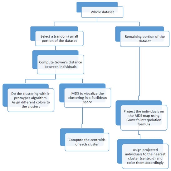
Figure 1.
Flowchart of the visualization algorithm.
Note that our proposal starts by clustering the individuals in the original space, and next, we use MDS to visualize the clustering in the Euclidean space. For that reason we use a clustering algorithm able to cope with mixed data, k-prototypes (although other methods can be used [3,4]). Another possibility would be to start with the MDS representation and next do the clustering on the Euclidean space using k-means clustering. In any case, when working with large datasets, a “fast” MDS is required in order to reduce both computational time and memory use. Thus, in any case, the idea of applying the methodology to a small portion of the data and to project the remaining individuals on the MDS-map remains. In this work, we explore the former; that is, we cluster the individuals in the original space instead of doing the clustering on the MDS-map, since an additional motivation was to incorporate Gower’s distance in the k-prototypes clustering algorithm.
The performance of our proposal was evaluated through a simulation study based on a real dataset of weighted and mixed data that came from the Survey of Health, Ageing and Retirement in Europe (SHARE), carried out in 19 countries. The analysis was applied to 60,020 individuals, who represent a target population of more than 124 million Europeans aged 55 years or over.
The work proceeds as follows: In Section 2 we review weighted MDS; in Section 3 we present the proposed methodology; in Section 4.1 we apply the method to data coming from SHARE database; Section 4.2 contains the simulation studies; and we conclude in Section 5.
2. Materials and Methods
In this section we give a general overview of classical MDS for weighted mixed data, introduce some useful notation and present Gower’s interpolation formula.
The purpose of MDS is to construct a set of points in a Euclidean space whose interdistances are either equal (classical MDS) or approximately equal (ratio, interval or ordinal MDS) to those in a given matrix of dissimilarities, so that the interpoint distances approximate the interobject dissimilarities. That is, given an matrix , where is the squared dissimilarity between objects , for , the objective of MDS is to search for a configuration of n points on a set of orthogonal axes, so that the -distances between the coordinates of these n points coincide with the corresponding entries in . These coordinates are called a Euclidean configuration/map/representation or MDS configuration/map/representation of . Several possible measures of approximation between interpoint distances and interobject dissimilarities can be used, each yielding a different MDS configuration. In this work, these coordinates are obtained via spectral decomposition. General contextual references are [5,6,7,8].
Sample surveys often employ multistage sampling schemes which involve unequal selection probabilities at some or all stages of the sampling process. We refer to this situation as a weighted context, where each individual can represent a population group of different size. In this framework, classical methods of data analysis which assume simple random sampling may no longer be valid, and weighting may appear as the only or best alternative. Albarrán et al. (2015) [9] reviewed the extension of classical MDS concepts to the weighted context.
2.1. Weighted MDS
Let be np-dimensional vectors which contain the observations or measurements of p variables for n different individuals and be the matrix of squared distances between n individuals, with entries , . Remember that the information contained in the p variables can be either of a quantitative or qualitative nature, or both, hence it is crucial to select an appropriate dissimilarity function in the computation of in order to incorporate all the statistical information contained in the data.
Additionally, since each individual in the dataset can represent a group of a different size of the target population (weighted context), we have a vector of weights , such that , for , and , where is the vector of 1 s. Note that in the case of simple random sampling—that is, when each individual in the dataset represents a group of the same size of the target population—, for , and classical MDS formulae are recovered.
Suppose that we are interested in obtaining an MDS representation of , provided that satisfies the Euclidean requirement.
Given , we define an diagonal matrix , whose diagonal is the vector of weights, and is the -centering matrix, where is the identity matrix.
The -centering matrix is an orthogonal projector with respect to , idempotent (that is, ) and self-adjoint with respect to (that is, ).
In the weighted context, the doubly -centered inner product matrix is given by
whose standardized version is given by
which is called standardized inner product matrix. The condition that satisfies the Euclidean requirement is equivalent to imposing that is positive semidefinite, which means that there exists a matrix such that . In the weighted context, is called a -centered Euclidean representation of and satisfies the following two properties:
- (a)
- .
- (b)
- The squared -distances between the rows of coincide with the corresponding entries in ; that is, for each pair of individuals , we have that where is the i-th row of .
Matrix is the -weighted MDS representation of and is computed by means of the spectral decomposition of matrix defined in Equation (1). That is, given , where is a diagonal matrix with the eigenvalues of , ordered in descending order, and is the corresponding matrix of eigenvectors (in column),
whose rows are the principal coordinates of n individuals, and its columns are the principal axes of this representation.
2.2. Gower’s Distance
Gower’s similarity coefficient [10] is one of the most popular similarity measures and perhaps the easiest way to obtain a distance measure when working with mixed data. It is the Pitagorean sum of three similarity coefficients, one for each type of variable. In particular, it uses Jaccard’s coefficient for binary variables, the simple matching coefficient for multi-state categorical variables and range-normalized city block distance for quantitative variables. Given two p-dimensional vectors and , Gower’s similarity coefficient is defined as:
where is the number of quantitative variables, is the range of the h-th quantitative variable, a is the number of positive matches, d is the number of negative matches for the binary variables, is the number of matches for the multi-state categorical variables and . The entries of matrix are computed as:
and Gower (1971) [10] proved that Equation (3) satisfies the Euclidean requirement.
Other metrics for mixed data can be considered, although the k-prototypes algorithm should be modified accordingly. For instance, a more robust metric that can overcome some of the shortcomings of Gower’s is related metric scaling (RelMS) by Cuadras (1998) [11], which was used in [9] to obtain robust profiles in weighted and mixed datasets. However, in this work, we prefer to illustrate our methodology by using Gower’s metric due to the computational complexity of RelMS.
2.3. Gower’s Interpolation Formula
A very useful tool to project new data points onto a given MDS configuration is Gower’s interpolation formula [8], which was extended to the weighted context by [12]. The following proposition can be derived from the Theorem 1 in [12]. This formula is a key tool in the visualization algorithm that we propose.
Proposition 1.
Let be a set of n individuals; a vector of weights, such that , for , and ; and be a matrix of squared distances between the n individuals satisfying the Euclidean requirement and the -weighted metric scaling representation of .
Given a new individual for whom the squared distances to n individuals of are known, , its principal coordinates can be computed as:
where is a row vector containing the diagonal elements of , , and is the diagonal matrix containing the eigenvalues of matrix defined in (1).
Proof.
The squared distance between the individual and any individual is given by
In matrix notation, we have that
Post multiplying expression (5) by and after operating, we have that:
Note that since and . Therefore, the principal coordinates of individual are given by:
since from Formula (2) we have that . □
3. Methodology
In this section we discuss a methodology for visualizing profiles for large datasets of weighted and mixed data.
Among all the approaches proposed for visualizing data, MDS is one of the most common techniques. However, we find the classical MDS algorithm a limited tool when visualizing large datasets, since it requires very large CPU time or large computing memory when dealing with large distance matrices. Delicado and Pachón-García (2020) [13] showed both: that the time needed to compute MDS as a function of the sample size increases notably when using cmdscale() R function (in stats package by R Development Core Team) and that at least 400 MB of RAM memory is required to store the distance matrix when there are 10,000 observations.
There have been several attempts to solve the scalability problem, such as steerable multidimensional scaling [14], incremental MDS [15], relative MDS [16], FastMap [17], MetricMap [18], landmark MDS [19], the diagonal majorization algorithm [20] and uniform manifold approximation and projection [21]. SteerMDS proposed by Williams et al. [14] is based on a spring-mass model, introduced by Chalmers [22] (see also [23] for a sampling-based variant of the algorithm). These methods calculate lower-dimensional coordinates by iteratively minimizing a cost or stress function that is proportional to the distance between the current coordinates and the given dissimilarities. Incremental MDS is similar to the previous methods, although it focuses on overall shape instead of local details. Relative MDS combines MDS with the learning vector quantization clustering method. FastMap, MetricMap and Landmark MDS approximate classical MDS by solving MDS for a subset of the data and fit the remainder to the solution. Platt [24] studied these methods and concluded that Landmark MDS was the fastest and most accurate of the them. The diagonal majorization algorithm is a modification of the Guttman majorization algorithm [25] that is used to minimize the stress function, and is able to save computing time taking into account several factors (see [26]). Finally, the uniform manifold approximation and projection is a learning technique for dimension reduction that can be used for visualization, which is indirectly related to MDS and more closely to Isomap.
The visualization method that we propose is based on classical MDS applied to a random portion of the dataset plus the projection of the remaining individuals via Gower’s interpolation formula. Thus, our proposal shares the idea behind several of the existing methods of applying MDS to a portion of the dataset, but differs from them in the projection tool used to obtain the final MDS representation.
3.1. The Visualization Algorithm
We start by summarizing the proposed method, and later we remark on some important aspects concerning the clustering algorithm and the feasible implementation of Gower’s interpolation formula.
The starting point of the algorithm is a large dataset of weighted and mixed data; that is, our dataset was composed of several variables of different natures (binary, multi-state categorical and numerical variables) plus a weighting variable containing the individual weights. Remember that weights are given exogenously and are related to the survey sampling technique. No pre-processing of the data is needed, except for the normalization of weights to sum to 1.
- Select a small random sample, using the weights to produce a more informative sample, that is, trying to follow as much as possible the sampling scheme. Depending on the size of dataset, this selection can be 2.5, 5 or 10% of total observations. Let us denote this small sample by , where n is the number of individuals and p the number of variables.
- Compute the distance matrix between the rows of using Gower’s distance Formula (3).
- Carry out the k-prototypes clustering algorithm in order to find the different clusters and label the individuals accordingly. Determine the number of clusters in the dataset by the “elbow” rule.
- Obtain the principal coordinates of the labeled individuals through weighted MDS.
- Compute the representatives (or centroids) of the clusters. This can be done by calculating the weighted mean or weighted median of those point-coordinates belonging to the same cluster in the MDS configuration.
- Project the rest of the individuals (the remaining 97.5, 95 or 90%) onto the MDS configuration using Gower’s interpolation formula.
- Finally, from the MDS configuration, assign the new points to an existing cluster based on the closest centroid (according to Euclidean distance) and label/color them accordingly.
Once all points have been assigned to a cluster, it is possible to visualize the clusters on the MDS configuration, and thus, to see the proximities between them. Finally, a profile is defined as the “average” member of each cluster. To do so, for categorical variables the mode can be computed and the mean and the median are good options for quantitative variables.
3.2. Some Important Remarks
Next, we introduce a few observations on the steps presented above.
3.2.1. On the Clustering Algorithm
Classical hierarchical clustering can handle also mixed data by using Gower’s coefficient. However, it is well known that it struggle as sample size increases. Reference [2] proposed a clustering algorithm called k-prototypes which is quite efficient, , where n is the number of observations, k the number of clusters and T the number of iterations; and it has been previously used by [27] for profile construction. The k-prototypes algorithm is based on a dissimilarity measure that takes into account both quantitative and categorical variables. Let be the variables available in the dataset, where stands for a quantitative variable and for a categorical one; then the dissimilarity between two individuals can be measured by
where for and for , and is a coefficient that measures the influences of numeric and categorical variables. Note that when , clustering only depends on numeric variables.
As it happens in any non-hierarchical clustering method, the number of clusters, k, must be determined in advance. To do so, a variety of techniques exist, and sometimes determining the optimal number of clusters is an inherently subjective measure that depends on the goal of the analysis. Due to the large size of the dataset, we decided to use the “elbow” method, instead of the average silhouette width or other time-consuming criteria. To apply the “elbow” method, we ran the algorithm for different values of k and calculated the cost function for each run. Then, we plotted the cost function in a line graph; and the point where a turning point (or “elbow”) was observed, that is, the point at which the cost function levels off, was selected as the optimal k value. Recently, Aschenbruck and Szepannek (2020) [28] examined the transferability of cluster validation indices to mixed data and evaluated them through simulation studies. They concluded that the average silhouette width was the most suitable with respect to both runtime and determination of the correct number of clusters. However, these conclusion rely on rather small datasets (≤400 individuals).
In this work, we introduce two particularities to the k-prototypes algorithm so that it can cope with Gower’s distance and weighted datasets.
First, instead of the measure described in (6), we used Gower’s distance Formula (3), which is a very popular dissimilarity measure for mixed data and satisfies the Euclidean requirement [10]. The second particularity introduced refers to weighted datasets. Since the ultimate difference from the standard algorithm is in centroid calculation, weighted averages of quantitative variables and weighted modes of categorical variables are used, instead of standard means and modes.
In what follows, we summarize the adapted version of the k-prototypes algorithm:
- Initial prototypes selection. Select k distinct individuals from the dataset as the initial centroids.
- Initial allocation. Each individual of the dataset is assigned to the closest prototype’s cluster, according to distance (3).
- Reallocation. The prototypes for the previous and current clusters of the individuals must be updated, taking into account individual weights. This repeats until there is no reallocation of individuals.
Some authors pointed out possible inaccurate clustering results when using Hamming distance and proposed other alternatives ([29,30]). In our simulations, we did not experiment with such situations (see Section 4.2 for graphical representations of the cost function). However, we propose to adapt the k-prototypes algorithm, although its convergence properties in combination with using Gower’s distance were not further investigated.
3.2.2. On Gower’s Interpolation Formula
As mentioned before, MDS’s final configuration is obtained by projecting the remaining observations via Gower’s interpolation formula on the initial configuration. But how can this be implemented in a feasible way? The idea is the following:
We call the remaining observations after selecting .
- Split row-wise into ℓ partitions , equally sized, with perhaps the exception of , which can be smaller. The number of partitions is set to be , where is the size of the largest distance matrix that a computer can calculate efficiently [13].
- Apply Gower’s interpolation formula to each matrix () and store the coordinates. The application of Gower’s interpolation formula to a matrix whose rows are m “new” individuals is rather straightforward from Formula (4). With the same notation as in Section 2.3, let be the matrix whose rows contain the squared distances of the “new” m individuals to the n individuals of . Then, the principal coordinates of these “new” m individuals can be computed by:where is a vector of ones.
This is simple, but strongly advantageous, since one of the main problems in MDS is memory consumption when computing distance matrices. Gower’s interpolation formula allows us to iteratively get the MDS configurations without facing memory problems, because we are reducing the size of the corresponding ℓ matrices that contain the squared distances to the n individuals of the existing MDS configuration. This aspect is studied in Section 4.2.
3.3. R Functions
There are several ways to perform metric MDS with R (see the MASS package for non-metric methods via the isoMDS function). In the following, we list them with their corresponding packages within parentheses:
- cmdscale (stats by R Development Core Team),
- pcoa (ape by [31]),
- dudi.pco (ade4 by [32]),
- smacofSym (smacof by [33]),
- wcmdscale (vegan by [34]),
- pco (labdsv by [35]),
- pco (ecodist by [36]).
All the functions listed above require a distance matrix as the main argument to work with. In case data are not in the distance/dissimilarity matrix format, R-functions dist, daisy and gower.dist may be of help. Moreover, some of the previous packages provide their own functions for calculating distances.
With respect to MDS configurations, the wcmdscale() function is used in this work. It is based on function cmdscale (base package of R—stats) and it can use point weights. Points with high weights will have stronger influences on the result than those with low weights. Setting equal weights will give ordinary multidimensional scaling.
Concerning the k-prototypes algorithm, the R package clustMixType by [37] contains the function kproto() needed to perform this technique. As mentioned before, we modified this function to achieve our desired goal, that is, to cope with Gower’s distance and weighted datasets.
4. Results
In this section we present a real data application and a simulation study to evaluate the performance of the visualization algorithm.
4.1. Application
Prior to analyzing the performance of the proposed methodology, we applied the algorithm described in Section 3 to a dataset from the Survey of Health, Ageing and Retirement in Europe (SHARE). SHARE is a research infrastructure, formed by a panel database of micro data, for studying the effects of health, social, economic and environmental policies over the lifetimes of European citizens and beyond. It was founded in 2002 and is coordinated centrally at the Munich Center for the Economics of Aging (MEA), the Max Planck Institute for Social Law and Social Policy (Munich, Germany). The SHARE interview is ex-ante harmonized and all aspects of the data generation process, from sampling to translation, and from fieldwork to data processing, have been conducted according to strict quality standards. As a result, SHARE has the advantage of encompassing cross-national variations in public health and socioeconomic living conditions of European individuals, and becoming a major pillar of the European research area, with over 9000 researchers registered as SHARE users. See their website http://www.share-project.org/ for further details. This work uses Wave 6 of SHARE, which was conducted in 2015 in 18 European countries and Israel. It asked questions ranging from an individual’s financial situation to his/her self-perception of health.
4.1.1. Description of the Dataset
The dataset to be analyzed consists of 60,020 observations and 13 variables, and includes a weighting variable that scales to represent over 124 million elderly individuals in Europe. Descriptions of variables are in Table 1. It is important to remark that the last four correspond to health and wellbeing indexes and were not in the original dataset, but created by [27] from the aggregations of 30 variables. Higher values of the indices correspond to situations of greater vulnerability. Although the process of creating those indices and other details about the dataset are described in their work, here we give a brief summary of the indices for better interpretation of the profiles.

Table 1.
Descriptive variables included in the analysis and their possible values or categories.
The dependency index summarizes the loss of personal autonomy. It includes variables that reflect difficulties in performing activities of daily living, instrumental activities of daily living, mobility limitations and so on.
The self-perception of health index is quite a subjective measure that captures some aspects of subjective wellbeing. This index includes variables related to what an individual thinks about their health rather than their physical reality, including how satisfied the interviewee is with their life, whether they are feeling depression, etc.
The physical health and nutrition index captures the risk of an individual to suffering or developing serious health problems. It contains information related to body mass index, grip strength, nutrition and chronic conditions of the individual.
The mental agility index captures the mental acuteness of the respondents and is related to cognitive functions. It contains the results of tests around numeracy, orientation and linguistic fluency.
Next, we proceed with the visualization and construction of the profiles for this dataset of weighted and mixed data.
4.1.2. Visualization of Profiles and Findings
The result of applying the visualization algorithm is shown in Figure 2. In order to select the number of clusters, the algorithm was run for . The cost function showed an “elbow” at around or . We investigated having 3 or 4 profiles and selected , since led to overly broad results. Panel (a) contains the MDS configuration based on Gower’s interpolation formula computed from a portion of of the data. Red triangles correspond to the mapped points of the random selection, and gray crosses stand for the projected ones. In panel (b) we show the pictorial representation of the clusters, where blue triangles stand for cluster centroids and circles represent their confidence regions, whose radii were computed as the 90th percentile of the (Euclidean) distance between each point and the corresponding centroid. We can observe beforehand two distinct groups of individuals, that is, a set of points grouped on the left (cluster 3) and another bunch of crowded points on the right, which splits into three small clusters. As will be seen later, cluster 3 corresponds to the least disadvantaged profile, whereas clusters 2 and 4 contain the most vulnerable individuals, according to the descriptive variables.
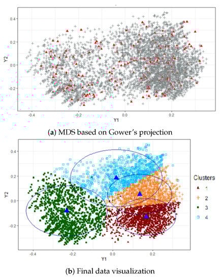
Figure 2.
Visualization of profiles. MDS based on Gower’s projection and final data visualization.
When original variables (and not just a matrix of distances or similarities) are available, it may be of interest to determine the influences of these original variables on the MDS dimensions, i.e., to determine which variables explain the most the homogeneity within groups. It was therefore necessary to calculate some correlation coefficient (or association measure) between the principal coordinates and the variables. We used Pearson’s correlation coefficient for continuous variables, Spearman’s correlation coefficient for ordinal variables and Cramer’s V measure of association for nominal variables. Results are shown in Table 2, where it can be seen that categorical variables, such as gender, job (Employment status), fdistress (household in financial distress) and paybene (household receives benefits or has payments) have great influences on the axes. For instance, the first principal coordinate is mostly determined by the variables job (employment status) and paybene (household receives benefits or has payments), whereas fdistress (household in financial distress) and gender are influential to the second and third principal coordinates. Quantitative variables do not seem to have many impacts on the axes, although the variable mental (mental agility index) influences the second coordinate somewhat. This was expected somehow, since Gower’s metric tends to give more weight to qualitative variables.
Table 2.
Correlations/associations among the original variables and the first three principal axes.
A graphical way to see the influences of the original variables on the construction of the profiles is to assign colors to the categories of the original variables (or groups of values, in the case of the quantitative ones) and represent the individuals colored accordingly in the MDS configuration. In Figure 3 we show the most representative projections of the MDS configuration regarding those variables more correlated/associated with the principal axes.
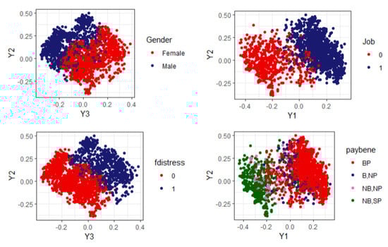
Figure 3.
MDS representation. Influential variables.
In the following we summarize the main characteristics of the four estimated profiles shown in Figure 2 (right panel). The results were acquired by taking the weighted mode for qualitative variables and the weighted mean and median for quantitative ones. See also Figure 4 and Figure 5 and Table 3.
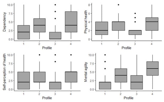
Figure 4.
A boxplot distribution of the indices by profile.
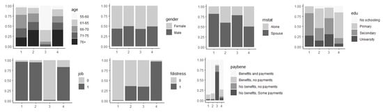
Figure 5.
Distribution of descriptive variables by profile.
Table 3.
Summary statistics of the variables used to create the profiles, per profile.
- P1:
- This included 30.48% of respondents, representing more than 37.89 million people; 56.56% of them were female, equally likely to belong to any age bracket, although more than 50% were under 71 years old; 55.18% were secondary-school-educated and more than 75% had secondary or university study behind them; not working; lived with a partner; health-related benefits and payments; wellbeing index mean values around 2–2.26 and median values of 2.
- P2:
- This included 22.76% of respondents, representing more than 28.29 million people; 50.26% of them were female; more than 50% of them were 70 years old or older; 47.80% were primary-school-educated and more than 75% were primary or secondary-school-educated; not working; lived with a partner; health-related benefits and payments; wellbeing index mean values around 3–4 and median values 2–4.
- P3:
- This included 26.82% of respondents, representing more than 33.34 million people; 57.27% female; 59.95% were between 55–65 years old and more than 80% were under 66 years old; around 70% were secondary-school-educated or university-educated; working; lived with a partner; no health-related benefits, some payments; least vulnerable group, wellbeing index mean values around 1.4–2.20, median values 0–2.
- P4:
- This included 19.94% of respondents, representing more than 24.78 million people; 51.35% female; 40.82% were 76 years old or older and more than 50% were older than 70 years old; low education (more than 75% were primary-school-educated or not at all); not working; likely lived alone or with a partner; health-related benefits and payments; 96.69% in financial distress; most vulnerable group, wellbeing index mean values around 3.4–5.4 and median values 4–6.
From the previous description we can sort the profiles from the most to the least disadvantaged, in terms of levels of health and socioeconomic wellbeing. In particular, P4 defines the group with the lowest levels of health and wellbeing, closely followed by P2. On the other hand, P1 defines a medium–low social vulnerability profile and P3 a profile of low risk of social vulnerability.
From Figure 4 and Table 3 we observe that profiles P4 and P2 more resemble each other compared to both other profiles across “dependency,” “mental agility” and “physical health,” whereas “self-perception of health” is more balanced. Remember that higher values of the indices correspond to situations of greater vulnerability.
P2 and P4 are the most vulnerable, although P2 is still better than P4. These profiles are especially vulnerable, since they have high percentages of individuals belonging to the 76 years or older group and they rank mostly bad in the indices, mainly due to the loss of physical or mental/intellectual autonomy produced by gradual aging. However, P4 is the one that ranked worst in all wellbeing indices, with mean differences of 0.31–1.39 points with respect to P2. Moreover, people in P4 were more likely to live alone than people in P2 (49.95% in front of 39.81%). Therefore, people in P4 were of the type that require more assistance and or extensive help in order to carry out common everyday actions. Additionally, we see that 96.69% of households in P4 were in financial distress, in front of 63.88% of the households in P2. Still comparing P2 and P4, another interesting finding is that the P4 individuals were more pessimistic with respect to their health. At least, this is what the distribution of the “self-perception of health” index seems to indicate (with a median difference of three points). This variable expresses what individuals think about their health: whether they are satisfied with their life, feeling depression, etc.
Clearly, the least disadvantaged group was P3, which heavily skewed towards younger individuals, since almost 60% of the individuals were aged between 55 and 60, and those over 76 made up less than 5% of this profile. In addition, 57.27% of them were women, and they tend to work until an advanced age. In addition, the indices indicate good health for this group, which may be related to the fact that continuing working in later life has been proved to be correlated with positive health outcomes [38]. Low values in wellbeing indices are consistent with the fact that people in this profile have no health-related benefits.
Finally, we see that education is one of the factors that most influences the profiles’ differences. Notice that most disadvantaged profiles have in common lower education levels (secondary, primary or none), whereas the most advantaged always have a high percentage of members who attended university. This finding supports the idea that society’s disparities are explained by differences in education among individuals. Education is often used as a proxy for socioeconomic status and its impact on later-life health outcomes is well researched [39,40].
4.1.3. Profiles across Europe
The variable “country,” which represents the country of residence of the individuals, was not included in the process described so far. However, it seemed interesting to see how the profiles are distributed across Europe, particularly for the most disadvantaged ones. Thus, for each country we computed the percentage of people belonging to each profile. Results are shown in Figure 6, where it can be seen that a combination of the least disadvantaged profiles is predominant in most European countries, except for Portugal, Estonia and Poland.
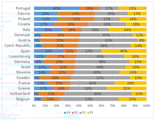
Figure 6.
Distribution of P1–P4 profiles by country.
A more interesting question is to find out whether SDG-3 of United Nations 2030 Agenda, that is, to ensure healthy lives and promote wellbeing for all at all ages, is fulfilled in these developed countries. To do so, we analyzed the percentages of the most disadvantaged profiles in these EU countries and found that they are concentrated in the Southern, Central and Eastern European countries. In particular, in countries such as Portugal, Spain, Italy and Poland it is estimated that over 20% of their population of 55 years old or older belong to P4. Regarding P2, it is estimated to be over 20% in 66.6% of the EU countries, geographically distributed in Central–Eastern European countries.
4.2. Simulation Study
Recall from Section 3 that we introduced Gower’s interpolation approach as a way to solve the scalability problem. However, is this true? Have we dealt successfully with the problem? We consider those questions next. The aim of this section is to evaluate the discrepancies between two MDS configurations, the classical one computed from the complete dataset and the one obtained with our algorithm. Besides, we analyze the time required to compute both configurations.
In this simulation study, the starting point is the dataset; hence, the computing times reported in this work are not comparable with those reported in [1], where the starting points were the first two principal coordinates.
4.2.1. Design of the Simulation Study
The analysis was carried out on samples of the dataset used in Section 4.1, and it was structured as follows:
- Sample sizes. To evaluate the elapsed time, a total of nine different sample sizes were used: n = 500, 1000, 5000, 10,000, 20,000, 30,000, 40,000, 50,000 and 60,000. Discrepancies between two MDS configurations were evaluated through a total of six different sample sizes: n = 500, 1000, 2000, 3000, 4000 and 5000.
- Portion of data. Recall that the first step of the algorithm was to select a small sample from the data. We wished to see whether there exists a significant difference in using 2.5, 5 or 10% as the initial portion.
- Each scenario was the combination of a sample size and a portion of data and was repeated 100 times.
For each repetition, we computed elapsed time; the errors in configuration eigenvalues, measured in terms of mean squared error (MSE); and the cophenetic correlation between Euclidean configurations, as a measure of distortion between two distance matrices [41].
We used a personal computer to run the simulation analysis, whose technical specifications were: computer processing unit: Intel®; core™ i5-4200U CPU @ 1.60 GHz 2.30 GHz; RAM: 4 GB (Santa Clara, CA, USA).
Table 4.
Time required to compute weighted MDS configurations (in seconds).
Table 5.
Discrepancies through eigenvalues (MSE) and Euclidean configurations (cophenetic correlation).
4.2.2. Time to Compute MDS
As stated before, in this section we analyze the divergence of the time required to compute MDS configurations when interpolating data points and when using all points (complete MDS from now on) to construct the coordinates. Table 4 contains the simulation study results. Clearly, we see that MDS based on Gower’s interpolation was, by far, the fastest one. Note that the table does not display any result for the complete MDS approach from observations onward. This was because of memory limitation problems. It could not even store the distance matrix. Nevertheless, we see that for small sample sizes we obtained a greater elapsed time for the complete MDS case, although we were not considering the time required to get the distance matrix (if we considered this, the difference would become even larger). As sample size increases, so do the time and memory needed. For example, for sample sizes of 500 to 1000, the elapsed time was almost six times higher for the complete MDS than for Gower’s approach. Another observation is that as sample size increases, it is more interesting to consider a portion of 2.5 or 5% rather than 10%. We will see in the next section whether there is a significant difference in choosing 2.5% instead of 10%.
4.2.3. Discrepancies in MDS Configurations
Here we compare the distortion of both MDS configurations by calculating the cophenetic correlation between them. That is, we want to know how different the configuration obtained through Gower’s interpolation formula is from the classical MDS (complete MDS). We also analyze how much the eigenvalues of both approaches differ by means of the mean square error (MSE), computed on the normalized positive eigenvalues of the two MDS configurations. As stated before, due to memory limitations, we could not do the comparisons for sample sizes greater than observations. Results are shown in Table 5, where we can see, first, that the normalized eigenvalues do not differ significantly (average MSE of 0.045 and median of 0.034), and second, that inter-distances between both configurations are preserved (average cophenetic correlation of 0.789 and median of 0.824). Overall, this simulation study reveals that discrepancies between configurations decrease as the sample size increases, and that, for a given sample size, they tend to decrease when we consider a higher sample portion. Although one can think of selecting a greater sample portion to reduce them, we must keep in mind that this requires more time to get the final MDS configuration.
4.2.4. Cost Function
Finally, we illustrate the convergence of the cost function of the k-prototypes algorithm, for and several of the scenarios described above. In Figure 7 we depict the mean and median values of the corresponding cost functions for which convergence was achieved in a rather small number of iterations.
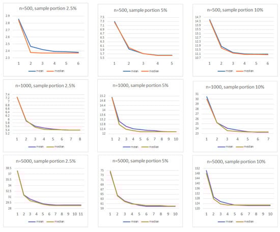
Figure 7.
Cost function mean and median values.
5. Conclusions
In this paper we presented a methodology for visualizing profiles of large datasets of weighted and mixed data that combines two classical multivariate techniques, MDS and a clustering algorithm. The clustering algortihm is used to partition the individuals in the original space, and once individuals are labeled accordingly, MDS is used to visualize the clusters in a Euclidean space, where it is easier to explore the proximities among clusters. The scalability problem is solved by means of Gower’s interpolation formula. Finally, profiles are obtained as the “average” member of each cluster, where the mode is considered for categorical variables and the mean or the median for numerical ones.
In this work we have illustrated this methodology by means of the k-prototypes clustering algorithm, although other clustering procedures able to cope with mixed data can be used [4]. Additional motivations for using k-prototypes were to adapt it to the weighted context and to use Gower’s metric as the dissimilarity measure. However, some authors pointed out possible inaccurate clustering results when using Hamming distance and proposed other alternatives ([29,30]). However, we did not experiment with such situations in our case study.
We tested the procedure through a simulation study, where we evaluated computational costs (elapsed time, errors in configuration eigenvalues) and discrepancies between classical and Gower’s interpolated MDS configurations (cophenetic correlation). The results show that MDS based on Gower’s interpolation formula solves the main issue of classical MDS (high computational cost) with few errors.
We applied the proposed methodology to find several profiles of healthy life and wellbeing in the European Union, using the respondents to the Survey of Health, Ageing and Retirement in Europe survey data. We found that the most vulnerable group (people with the poorest health and wellbeing) contained elderly people who were less educated, living alone, had financial problems, had low personal autonomy and had impairments in cognitive abilities. This profile is more likely to be found in Southern and Eastern European countries.
Although Gower’s metric is widely used when dealing with mixed datasets, it presents several shortcomings. For example, it gives more weight to categorical variables than to quantitative ones; it does not take into account the possible associations or correlations between variables; and it is not robust against atypical data (see [9,42,43]).
An interesting direction for future research would be to consider other metrics, such as the hybrid dissimilarity coefficient by Jian and Song [30], and their modification of the k-prototypes algorithm, although it is more time consuming than the classical k-prototypes. Nevertheless, this hybrid dissimilarity still ignores the association between variables. Another possibility would be to use related metric scaling (RelMS) to tailor the metric and incorporate it into the clustering algorithm. RelMS was introduced in [11,44] and provides more robust and stable configurations than Gower’s, but it has a high computational cost, which should be reduced so that it can be workable for large datasets. Another interesting direction for future research would be to explore the possibility of combining our methodology with clustering algorithms based on archetype and archetypoid analysis, which focuses on extreme individuals instead of centroids ([45,46]).
Author Contributions
Conceptualization, A.G. and A.A.S.-B.; methodology, A.G.; software, A.A.S.-B.; validation, A.A.S.-B. and A.G., data curation, A.A.S.-B.; writing—original draft preparation, A.A.S.-B.; writing—review and editing, A.G.; supervision, A.G.; project administration, A.G.; funding acquisition, A.G. All authors have read and agreed to the published version of the manuscript.
Funding
This research was funded by the Spanish Ministry of Economy and Competitiveness, grant number MTM2014-56535-R; and the V Regional Plan for Scientific Research and Technological Innovation 2016–2020 of the Community of Madrid, an agreement with Universidad Carlos III de Madrid in the action of “Excellence for University Professors”.
Institutional Review Board Statement
Not applicable.
Informed Consent Statement
Not applicable.
Data Availability Statement
Original data can be downloaded from http://www.share-project.org/.
Acknowledgments
The authors are grateful to Pedro Delicado for his useful comments and suggestions.
Conflicts of Interest
The authors declare no conflict of interest.
References
- Paradis, E. Multdimensional scaling with very large datasets. J. Comput. Graph. Stat. 2018, 27, 935–939. [Google Scholar] [CrossRef]
- Huang, Z. Clustering large data sets with mixed numeric and categorical values. In Proceedings of the First Pacific Asia Knowledge Discovery and Data Mining Conference, Singapore, 23–24 February 1997; World Scientific: Singapore, 1997; pp. 21–34. [Google Scholar]
- Van de Velden, M.; Iodice D’Enza, A.; Markos, A. Distance-based clustering of mixed data. Wires Comput. Stat. 2018, 11, e1456. [Google Scholar] [CrossRef]
- Ahmad, A.; Khan, S.S. Survey of State-of-the-Art Mixed Data Clustering Algorithms. IEEE Access 2019, 7, 31883–31902. [Google Scholar] [CrossRef]
- Borg, I.; Groenen, P.J.F. Modern Multidimensional Scaling: Theory and Applications, 2nd ed.; Springer: New York, NY, USA, 2005. [Google Scholar]
- Cox, T.F.; Cox, M.A.A. Multidimensional Scaling, 2nd ed.; Chapman and Hall: Boca Raton, FL, USA, 2000. [Google Scholar]
- Krzanowski, W.J.; Marriott, F.H.C. Multivariate Analysis, Part 1, Volume Distributions, Ordination and Inference; Arnold: London, UK, 1994. [Google Scholar]
- Gower, J.C.; Hand, D. Biplots; Chapman and Hall: London, UK, 1996. [Google Scholar]
- Albarrán, A.; Alonso, P.; Grané, A. Profile identification via weighted related metric scaling: An application to dependent Spanish children. J. R. Stat. Soc. Ser. Stat. Soc. 2015, 178, 1–26. [Google Scholar] [CrossRef]
- Gower, J.C. A general coefficient of similarity and some of its properties. Biometrics 1971, 27, 857–874. [Google Scholar] [CrossRef]
- Cuadras, C.M. Multidimensional Dependencies in Ordination and Classification. In Analyses Multidimensionelles des Données; Fernández, K., Morineau, A., Eds.; CISIA-CERESTA: Saint-Mandé, France, 1998; pp. 15–25. [Google Scholar]
- Boj, E.; Delicado, P.; Fortiana, J. Distance-based local linear regression for functional predictors. Comput. Stat. Data Anal. 2010, 54, 429–437. [Google Scholar] [CrossRef]
- Delicado, P.; Pachón-García, C. Multidimensional Scaling for Big Data. 2020. Available online: https://arxiv.org/abs/2007.11919 (accessed on 23 July 2020).
- Williams, M.; Munzner, T. Steerable, progressive multidimensional scaling. In Proceedings of the Information Visualization, INFOVIS 2004, IEEE Symposium, Austin, TX, USA, 10–12 October 2004; pp. 57–64. [Google Scholar]
- Basalaj, W. Incremental multidimensional scaling method for database visualization. In Proceedings of the SPIE 3643, Visual Data Exploration and Analysis VI, San Jose, CA, USA, 25 March 1999. [Google Scholar] [CrossRef]
- Naud, A.; Duch, W. Interactive data exploration using MDS mapping. In Proceedings of the Fifth Conference: Neural Networks and Soft Computing, Zakopane, Poland, 6–10 June 2000; pp. 255–260. [Google Scholar]
- Faloutsos, C.; Lin, K. FastMap: A fast algorithm for indexing, data-mining, and visualization. In Proceedings of the ACM SIGMOD, San Jose, CA, USA, 23–25 May 1995; pp. 163–174. [Google Scholar]
- Wang, J.T.-L.; Wang, X.; Lin, K.-I.; Shasa, D.; Shapiro, B.A.; Zhang, K. Evaluating a class of distance-mapping algorithms for data mining and clustering. In Proceedings of the ACM KDD, San Diego, CA, USA, 15–18 August 1999; pp. 307–311. [Google Scholar]
- De Silva, V.; Tenenbaum, J.B. Global versus local methods for nonlinear dimensionality reduction. Adv. Neural Inf. Process. Syst. 2003, 15, 721–728. [Google Scholar]
- Trosset, W.M.; Groenen, P.J. Multidimensional scaling algorithms for large data sets interactive data exploration using MDS mapping. In Proceedings of the Computing Science and Statistics, Kunming, China, 7–9 December 2005. [Google Scholar]
- McInnes, L.; Healy, J.; Saul, N.; Großberger, L. UMAP: Uniform Manifold Approximation and Projection. J. Open Source Softw. 2018, 3, 861. [Google Scholar] [CrossRef]
- Chalmers, M. A linear iteration time layout algorithm for visualizing high dimensional data. Proc. IEEE Vis. 1996, 127–132. [Google Scholar] [CrossRef]
- Morrison, A.; Ross, G.; Chalmers, M. Fast Multidimensional Scaling through Sampling, Springs, and Interpolation. Inf. Vis. 2003, 2, 68–77. [Google Scholar] [CrossRef]
- Platt, J.C. FastMap, MetricMap, and Landmark MDS are all Nyström Algorithms. In Proceedings of the 10th International Workshop on Artificial Intelligence and Statistics, Bridgetown, Barbados, 6–8 January 2005; pp. 261–268. [Google Scholar]
- Guttman, L. A general nonmetric technique for finding the smallest coordinate space for a configuration of points. Psychometrika 1968, 33, 469–506. [Google Scholar] [CrossRef]
- Bernataviciene, J.; Dzemyda, G.; Marcinkevicius, V. Diagonal Majorizarion Algorithm: Properties and efficiency. Inf. Technol. Control 2007, 36, 353–358. [Google Scholar]
- Grané, A.; Albarrán, I.; Lumley, R. Visualizing Inequality in Health and Socioeconomic Wellbeing in the EU: Findings from the SHARE Survey. Int. J. Environ. Res. Public Health 2020, 17, 7747. [Google Scholar] [CrossRef] [PubMed]
- Aschenbruck, R.; Szepannek, G. Cluster Validation for Mixed-Type Data. Achives Data Sci. Ser. A 2020. [Google Scholar] [CrossRef]
- Foss, A.H.; Markatou, M.; Ray, B. Distance Metrics and Clustering Methods for Mixed-type Data. Int. Stat. Rev. 2018, 81, 80–109. [Google Scholar] [CrossRef]
- Jia, Z.; Song, L. Weighted k-Prototypes Clustering Algorithm Based on the Hybrid Dissimilarity Coefficient. Math. Probl. Eng. 2020, 5143797. [Google Scholar] [CrossRef]
- Paradis, E.; Claude, J.; Strimmer, K. APE: Analyses of phylogenetics and evolution in R language. Bioinformatics 2004, 20, 289–290. [Google Scholar] [CrossRef]
- Dray, S.; Dufour, A.B. The ade4 Package: Implementing the Duality Diagram for Ecologists. J. Stat. Softw. 2007, 22. [Google Scholar] [CrossRef]
- De Leeuw, J.; Mair, P. Multidimensional scaling using majorization: The R package smacof. J. Stat. Softw. 2009, 31, 1–30. [Google Scholar] [CrossRef]
- Oksanen, J.; Blanchet, F.G.; Friendly, M.; Kindt, R.; Legendre, P.; McGlinn, D.; Minchin, P.R.; O’Hara, R.B.; Simpson, G.L.; Solymos, P.; et al. Community Ecology Package, CRAN-Package Vegan. Available online: https://cran.r-project.org; https://github.com/vegandevs/vegan (accessed on 1 March 2020).
- Roberts, D.W. Ordination and Multivariate Analysis for Ecology. CRAN-Package Labdsv. Available online: http://ecology.msu.montana.edu/labdsv/R (accessed on 1 March 2020).
- Goslee, S.; Urban, D. Dissimilarity-Based Functions for Ecological Analysis. CRAN-Package Ecodist. Available online: https://CRAN.R-project.org/package=ecodist (accessed on 1 March 2020).
- Szepannek, G. ClustMixType: User-Friendly Clustering of Mixed-Type Data in R. R J. 2018, 10, 200–208. [Google Scholar] [CrossRef]
- Ney, S. Active Aging Policy in Europe: Between Path Dependency and Path Departure. Ageing Int. 2005, 30, 325–342. [Google Scholar] [CrossRef]
- Avendano, M.; Jürges, H.; MacKenbach, J.P. Educational level and changes in health across Europe: Longitudinal results from SHARE. J. Eur. Soc. Policy 2009, 19, 301–316. [Google Scholar] [CrossRef]
- Bohácek, R.; Crespo, L.; Mira, P.; Pijoan-Mas, J. The Educational Gradient in Life Expectancy in Europe: Preliminary Evidence from SHARE. In Ageing in Europe—Supporting Policies for an Inclusive Society; Börsch-Supan, A., Kneip, T., Litwin, H., Myck, M., Weber, G., Eds.; De Gruyter: Berlin, Germany, 2015; pp. 321–330. [Google Scholar] [CrossRef]
- Sokal, R.R.; Rohlf, F.J. The comparison of dendrograms by objective methods. Taxon 1962, 11, 33–40. [Google Scholar] [CrossRef]
- Grané, A.; Romera, R. On visualizing mixed-type data: A joint metric approach to profile construction and outlier detection. Sociol. Methods Res. 2018, 47, 207–239. [Google Scholar] [CrossRef]
- Grané, A.; Salini, S.; Verdolini, E. Robust multivariate analysis for mixed-type data: Novel algorithm and its practical application in socio-economic research. Socio-Econ. Plan. Sci. 2021, 73, 100907. [Google Scholar] [CrossRef]
- Cuadras, C.M.; Fortiana, J. Visualizing Categorical Data with Related Metric Scaling. In Visualization of Categorical Data; Blasius, J., Greenacre, M., Eds.; Academic Press: London, UK, 1998; pp. 365–376. [Google Scholar]
- Cutler, A.; Breiman, L. Archetypal analysis. Technometrics 1994, 36, 338–347. [Google Scholar] [CrossRef]
- Vinué, G.; Epifanio, I.; Alemany, S. Archetypoids: A new approach to define representative archetypal data. Comput. Statist. Data Anal. 2015, 87, 102–115. [Google Scholar] [CrossRef]
Publisher’s Note: MDPI stays neutral with regard to jurisdictional claims in published maps and institutional affiliations. |
© 2021 by the authors. Licensee MDPI, Basel, Switzerland. This article is an open access article distributed under the terms and conditions of the Creative Commons Attribution (CC BY) license (https://creativecommons.org/licenses/by/4.0/).